2. first steps in mupad - buecher.de · 2. first steps in mupad computer algebra systems such as...

2. First Steps in MuPAD

Computer algebra systems such as MuPAD are often used interactively. Forexample, you can enter an instruction to multiply two numbers and wait untilMuPAD computes the result and prints it on the screen.

After you call the MuPAD program, a session is launched. You find theinformation how to start the MuPAD program in the MuPAD installation in-structions for your operating system. MuPAD provides a help system whichyou can consult during a session to find details about system functions, theirsyntax, their parameters, etc. The following section presents an introduc-tion to MuPAD’s help system. Requesting a help page is probably the mostfrequently used command for the beginner. The section after that is aboutusing MuPAD as an “intelligent pocket calculator”: calculating with numbers.This is the easiest and the most intuitive part of this tutorial. Afterwardswe introduce some system functions for symbolic computations. The corres-ponding section is written quite informally and gives a first insight into thesymbolic features of the system.

After starting the program, you can enter commands in the MuPAD lan-guage. The system awaits your input when the MuPAD prompt appearson the screen. On a Windows or Macintosh system, the prompt is the •sign, while it is >> on UNIX platforms. We use the UNIX prompt in allexamples throughout the book. If you press the <Return> key under UNIXor Windows, this finishes your input and MuPAD evaluates the commandthat you have entered. Holding <Shift> while pressing <Return> only pro-vokes a linefeed and still leaves MuPAD in input mode. On a Macintosh,<Shift>+<Return> or <Enter> executes a command and <Return> onlyprovokes a linefeed. For all GUI versions, you can exchange the roles of<Return> and <Shift>+<Return> by choosing “Options” in the “View”menu and then clicking on “Enter only.”

8 2. First Steps in MuPAD

If you enter:

>> sin(3.141)

and then press <Return> (or <Enter>, respectively), the result

0.0005926535551

is printed on your screen. The system evaluates the usual sine function at thepoint 3.141 and returns a floating-point approximation of the value, similarto the output of a pocket calculator.

If you terminate your command with a colon, then MuPAD executes the com-mand without printing its result on the screen. This enables you to suppressthe output of irrelevant intermediate results. You can enter more than onecommand in one line. Two subsequent commands have to be separated bya semicolon or a colon, if the result of the first command is to be printed ornot, respectively:

>> diff(sin(x^2), x); int(%, x)

2 x cos(x2)

sin(x2)

Here x^2 denotes the square of x, and the MuPAD functions diff and intperform the operations “differentiate” and “integrate” (Chapter 7). The char-acter % returns the previous expression (in the example, this is the derivativeof sin(x2)). The concept underlying % is discussed in Chapter 12.

In the following example, the output of the first command is suppressed bythe colon, and only the result of the second command appears on the screen:

>> equations := {x + y = 1, x - y = 1}:>> solve(equations)

{[x = 1, y = 0]}

In the previous example, a set of two equations is assigned to the identi-fier equations. The command solve(equations) computes the solution.Chapter 8 discusses the solver in more detail.

In the terminal version of MuPAD (on UNIX systems), you can end thecurrent MuPAD session by entering the keyword quit:

>> quit

2.1 Explanations and Help 9

MuPAD versions with a graphical interface must be quit with the correspond-ing menu entry in the GUI.

2.1 Explanations and Help

If you do not know the correct syntax of a MuPAD command, you can obtainthis information directly from the online help system. For many MuPADroutines, the function info returns a brief explanation:

>> info(solve)solve -- solve equations and inequalities [try ?solve\for options]

>> info(ln)ln -- the natural logarithm

The help page of the corresponding function provides more detailed informa-tion. You can request it by entering help("name"), where name is the nameof the function. The function help expects its argument to be a string, whichare generated by double quotes " in MuPAD (Section 4.11). The operator ?is a short form for help. It is used without parenthesis or quotes:

>> ?solve

The layout of the help pages depends on the MuPAD version. In the followingexample, you can see a help page in ASCII format, like it is returned by theterminal version of MuPAD in response to ?solve:

solve – solve equations and inequalities

Introduction

solve(eq, x) returns the set of all complex solutions of an equation orinequality eq with respect to x.

solve(system, vars) solves a system of equations for the variables vars.

solve(eq, vars) is equivalent to solve([eq], vars).

solve(system, x) is equivalent to solve(system, [x]).

solve(eq) without second argument is equivalent to solve(eq, S) where Sis the set of all indeterminates in eq. The same holds for solve(system).


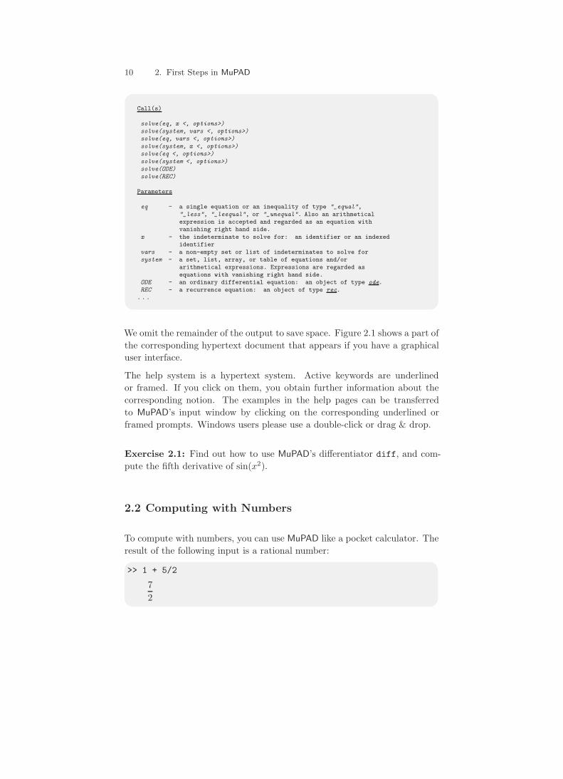
Call(s)

solve(eq, x <, options>)solve(system, vars <, options>)solve(eq, vars <, options>)solve(system, x <, options>)solve(eq <, options>)solve(system <, options>)solve(ODE)solve(REC)

Parameters

eq - a single equation or an inequality of type "_equal","_less", "_leequal", or "_unequal". Also an arithmeticalexpression is accepted and regarded as an equation withvanishing right hand side.

x - the indeterminate to solve for: an identifier or an indexedidentifier

vars - a non-empty set or list of indeterminates to solve forsystem - a set, list, array, or table of equations and/or

arithmetical expressions. Expressions are regarded asequations with vanishing right hand side.

ODE - an ordinary differential equation: an object of type ode.REC - a recurrence equation: an object of type rec.

. . .

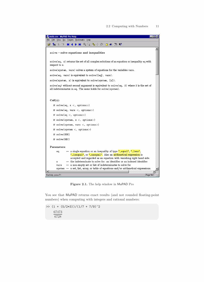
We omit the remainder of the output to save space. Figure 2.1 shows a part ofthe corresponding hypertext document that appears if you have a graphicaluser interface.

The help system is a hypertext system. Active keywords are underlinedor framed. If you click on them, you obtain further information about thecorresponding notion. The examples in the help pages can be transferredto MuPAD’s input window by clicking on the corresponding underlined orframed prompts. Windows users please use a double-click or drag & drop.

Exercise 2.1: Find out how to use MuPAD’s differentiator diff, and com-pute the fifth derivative of sin(x2).

2.2 Computing with Numbers

To compute with numbers, you can use MuPAD like a pocket calculator. Theresult of the following input is a rational number:

>> 1 + 5/2

72

2.2 Computing with Numbers 11

Figure 2.1. The help window in MuPAD Pro

You see that MuPAD returns exact results (and not rounded floating-pointnumbers) when computing with integers and rational numbers:

>> (1 + (5/2*3))/(1/7 + 7/9)^2

674736728


The symbol ^ represents exponentiation. MuPAD can compute big numbersefficiently. The length of a number that you may compute is only limited bythe available main storage. For example, the 123rd power of 1234 is a fairlybig integer:1

>> 1234^12317051580621272704287505972762062628265430231311106829\04705296193221839138348680074713663067170605985726415\92314554345900570589670671499709086102539904846514793\13561730556366999395010462203568202735575775507008323\84441477783960263870670426857004040032870424806396806\96865587865016699383883388831980459159942845372414601\80942971772610762859524340680101441852976627983806720\3562799104

Besides the basic arithmetic functions, MuPAD provides a variety of functionsoperating on numbers. A simple example is the factorial n! = 1 · 2 · · ·n of anonnegative integer, which can be entered in mathematical notation:

>> 100!93326215443944152681699238856266700490715968264381621\46859296389521759999322991560894146397615651828625369\7920827223758251185210916864000000000000000000000000

The function isprime checks whether a positive integer is prime. It returnseither TRUE or FALSE.

>> isprime(123456789)

FALSE

Using ifactor, you can obtain the prime factorization:

>> ifactor(123456789)

32 · 3607 · 3803

2.2.1 Exact Computations

Now suppose that we want to “compute” the number√

56. The problem isthat the value of this irrational number cannot be expressed as a quotientnumerator/denominator of two integers exactly. Thus “computation” canonly mean to find an exact representation that is as simple as possible. Whenyou input

√56 via sqrt, MuPAD returns the following:

1 In this printout, the “backslash” \ at the end of a line indicates that the resultis continued on the next line.


>> sqrt(56)

2√

14

The result of the simplification of√

56 is the exact value 2 · √14. In MuPAD,√14 (or, sometimes, 14^(1/2)) represents the positive solution of the equa-

tion x2 = 14. Indeed, this is probably the most simple representation of theresult. We stress that

√14 is a genuine MuPAD object with certain proper-

ties (e.g., that its square can be simplified to 14). The system applies themautomatically when computing with such objects. For example:

>> sqrt(14)^4

196

As another example for exact computation, let us determine the limit

e = limn→∞

(1 +

1n

)n

.

We use the function limit and the symbol infinity:

>> limit((1 + 1/n)^n, n = infinity)e

To enter this number in a MuPAD input, you have to use E or exp(1), whereexp represents the exponential function. MuPAD knows exact rules of ma-nipulation for this object. For example, using the natural logarithm ln wefind:

>> ln(1/exp(1))

−1

We will encounter more exact computations later in this tutorial.

2.2.2 Numerical Approximations

Besides exact computations, MuPAD can also perform numerical approxima-tions. For example, you can use the MuPAD function float to find a decimalapproximation to

√56. This function computes the value of its argument in

floating-point representation:

>> float(sqrt(56))

7.483314774


The precision of the approximation depends on the value of the global vari-able DIGITS, which determines the number of decimal digits for numericalcomputations. Its default value is 10:

>> DIGITS; float(67473/6728)

10

10.02868609

Global variables such as DIGITS affect the behavior of MuPAD and are alsocalled environment variables.2 You find a complete list of all environmentvariables in Section “Environment Variables” of the MuPAD Quick Refer-ence [Oev 03]. The variable DIGITS can assume any integral value between 1and 232 − 1:

>> DIGITS := 100: float(67473/6728); DIGITS := 10:10.02868608799048751486325802615933412604042806183115\338882282996432818073721759809750297265160523187

We have reset the value of DIGITS to 10 for the following computations. Thiscan also be achieved via the command delete DIGITS. For arithmetic oper-ations with numbers, MuPAD automatically uses approximate computationas soon as at least one of the numbers involved is a floating-point value:

>> (1.0 + (5/2*3))/(1/7 + 7/9)^2

10.02868609

Please note that none of the two following calls

>> 2/3*sin(2), 0.6666666666*sin(2)

results in an approximate computation of sin(2), since, technically, sin(2) isan expression representing the (exact) value of sin(2) and not a number:

2 sin (2)3

, 0.6666666666 sin (2)

2 You should be particularly cautious when the same computation is performedwith different values of DIGITS. Some of the more intricate numerical algorithmsin MuPAD employ the option “remember.” This implies that they store pre-viously computed values to be used again (Section 18.9), which can lead toinaccurate numerical results if the remembered values were computed with lowerprecision. To be safe, you should restart the MuPAD session using reset() be-fore increasing the value of DIGITS. This command clears MuPAD’s memory andresets all environment variables to their default values (Section 14.3).


(The separation of both values by a comma generates a special data type,namely a sequence, which is described in Section 4.5.) You have to usethe function float to compute floating-point approximations of the aboveexpressions:3

>> float(2/3*sin(2)), 0.6666666666*float(sin(2))

0.6061982846, 0.6061982845

Most arithmetic functions in MuPAD, such as sqrt, the trigonometric func-tions, the exponential function, or the logarithm, automatically return ap-proximate values when their argument is a floating-point number:

>> sqrt(56.0), sin(3.14)

7.483314774, 0.001592652916

The constants π and e are denoted by PI and E = exp(1), respectively.MuPAD can perform exact computations with them:

>> cos(PI), ln(E)

−1, 1

If desired, you can obtain numerical approximations of these constants byapplying float:

>> DIGITS := 100: float(PI); float(E); delete DIGITS:3.141592653589793238462643383279502884197169399375105\820974944592307816406286208998628034825342117068

2.718281828459045235360287471352662497757247093699959\574966967627724076630353547594571382178525166427

Exercise 2.2: Compute√

27 − 2√

3 and cos(π/8) exactly. Determine nu-merical approximations to a precision of 5 digits.

3 Take a look at the last digits. The second command yields a slightly less accurateresult, since 0.666 . . . is already an approximation of 2/3 and the rounding erroris propagated to the final result.


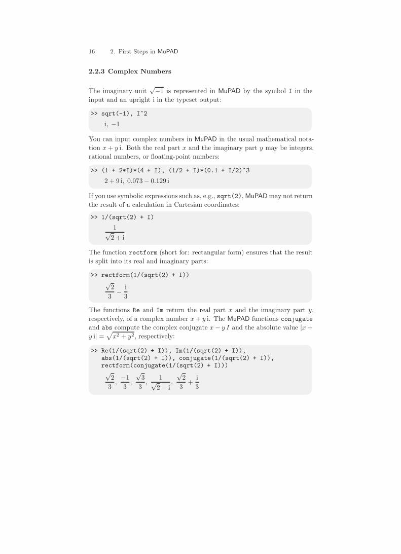
2.2.3 Complex Numbers

The imaginary unit√−1 is represented in MuPAD by the symbol I in the

input and an upright i in the typeset output:

>> sqrt(-1), I^2

i, −1

You can input complex numbers in MuPAD in the usual mathematical nota-tion x + y i. Both the real part x and the imaginary part y may be integers,rational numbers, or floating-point numbers:

>> (1 + 2*I)*(4 + I), (1/2 + I)*(0.1 + I/2)^3

2 + 9 i, 0.073− 0.129 i

If you use symbolic expressions such as, e.g., sqrt(2), MuPAD may not returnthe result of a calculation in Cartesian coordinates:

>> 1/(sqrt(2) + I)

1√2 + i

The function rectform (short for: rectangular form) ensures that the resultis split into its real and imaginary parts:

>> rectform(1/(sqrt(2) + I))√

23

− i3

The functions Re and Im return the real part x and the imaginary part y,respectively, of a complex number x + y i. The MuPAD functions conjugateand abs compute the complex conjugate x − y I and the absolute value |x +y i| =

√x2 + y2, respectively:

>> Re(1/(sqrt(2) + I)), Im(1/(sqrt(2) + I)),abs(1/(sqrt(2) + I)), conjugate(1/(sqrt(2) + I)),rectform(conjugate(1/(sqrt(2) + I)))√

23

,−13

,

√3

3,

1√2 − i

,

√2

3+

i3

2.3 Symbolic Computation 17

2.3 Symbolic Computation

This section comprises some examples of MuPAD sessions that illustrate asmall selection of the system’s power of symbolic manipulation. The math-ematical knowledge is contained essentially in MuPAD’s functions for differ-entiation, integration, simplification of expressions etc. This demonstrationdoes not proceed in a particularly systematic manner: we apply the systemfunctions to objects of various types, such as sequences, sets, lists, expressionsetc. They are explained in detail one by one in Chapter 4.

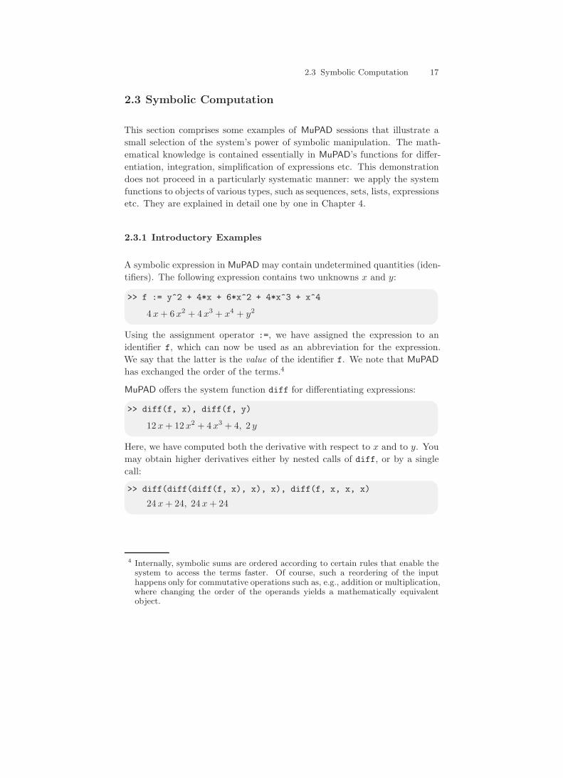
2.3.1 Introductory Examples

A symbolic expression in MuPAD may contain undetermined quantities (iden-tifiers). The following expression contains two unknowns x and y:

>> f := y^2 + 4*x + 6*x^2 + 4*x^3 + x^4

4 x + 6 x2 + 4 x3 + x4 + y2

Using the assignment operator :=, we have assigned the expression to anidentifier f, which can now be used as an abbreviation for the expression.We say that the latter is the value of the identifier f. We note that MuPADhas exchanged the order of the terms.4

MuPAD offers the system function diff for differentiating expressions:

>> diff(f, x), diff(f, y)

12 x + 12 x2 + 4 x3 + 4, 2 y

Here, we have computed both the derivative with respect to x and to y. Youmay obtain higher derivatives either by nested calls of diff, or by a singlecall:

>> diff(diff(diff(f, x), x), x), diff(f, x, x, x)

24 x + 24, 24 x + 24

4 Internally, symbolic sums are ordered according to certain rules that enable thesystem to access the terms faster. Of course, such a reordering of the inputhappens only for commutative operations such as, e.g., addition or multiplication,where changing the order of the operands yields a mathematically equivalentobject.


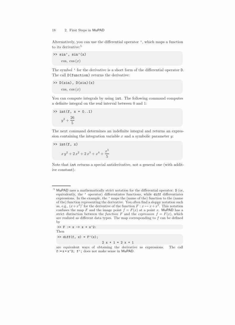
Alternatively, you can use the differential operator ’, which maps a functionto its derivative:5

>> sin’, sin’(x)

cos, cos (x)

The symbol ’ for the derivative is a short form of the differential operator D.The call D(function) returns the derivative:

>> D(sin), D(sin)(x)

cos, cos (x)

You can compute integrals by using int. The following command computesa definite integral on the real interval between 0 and 1:

>> int(f, x = 0..1)

y2 +265

The next command determines an indefinite integral and returns an expres-sion containing the integration variable x and a symbolic parameter y:

>> int(f, x)

x y2 + 2 x2 + 2 x3 + x4 +x5

5

Note that int returns a special antiderivative, not a general one (with addit-ive constant).

5 MuPAD uses a mathematically strict notation for the differential operator: D (or,equivalently, the ’ operator) differentiates functions, while diff differentiatesexpressions. In the example, the ’ maps the (name of the) function to the (nameof the) function representing the derivative. You often find a sloppy notation suchas, e.g., (x+x2)′ for the derivative of the function F : x �→ x+x2. This notationconfuses the map F and the image point f = F (x) at a point x. MuPAD has astrict distinction between the function F and the expression f = F (x), whichare realized as different data types. The map corresponding to f can be definedby>> F := x -> x + xˆ2:

Then

>> diff(f, x) = F’(x);

2 x + 1 = 2 x + 1are equivalent ways of obtaining the derivative as expressions. The callf:= x + x^2; f’; does not make sense in MuPAD.


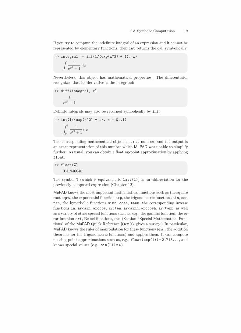
If you try to compute the indefinite integral of an expression and it cannot berepresented by elementary functions, then int returns the call symbolically:

>> integral := int(1/(exp(x^2) + 1), x)∫1

ex2 + 1dx

Nevertheless, this object has mathematical properties. The differentiatorrecognizes that its derivative is the integrand:

>> diff(integral, x)

1ex2 + 1

Definite integrals may also be returned symbolically by int:

>> int(1/(exp(x^2) + 1), x = 0..1)∫ 1

0

1ex2 + 1

dx

The corresponding mathematical object is a real number, and the output isan exact representation of this number which MuPAD was unable to simplifyfurther. As usual, you can obtain a floating-point approximation by applyingfloat:

>> float(%)

0.41946648

The symbol % (which is equivalent to last(1)) is an abbreviation for thepreviously computed expression (Chapter 12).

MuPAD knows the most important mathematical functions such as the squareroot sqrt, the exponential function exp, the trigonometric functions sin, cos,tan, the hyperbolic functions sinh, cosh, tanh, the corresponding inversefunctions ln, arcsin, arccos, arctan, arcsinh, arccosh, arctanh, as wellas a variety of other special functions such as, e.g., the gamma function, the er-ror function erf, Bessel functions, etc. (Section “Special Mathematical Func-tions” of the MuPAD Quick Reference [Oev 03] gives a survey.) In particular,MuPAD knows the rules of manipulation for these functions (e.g., the additiontheorems for the trigonometric functions) and applies them. It can computefloating-point approximations such as, e.g., float(exp(1))= 2.718..., andknows special values (e.g., sin(PI)= 0).


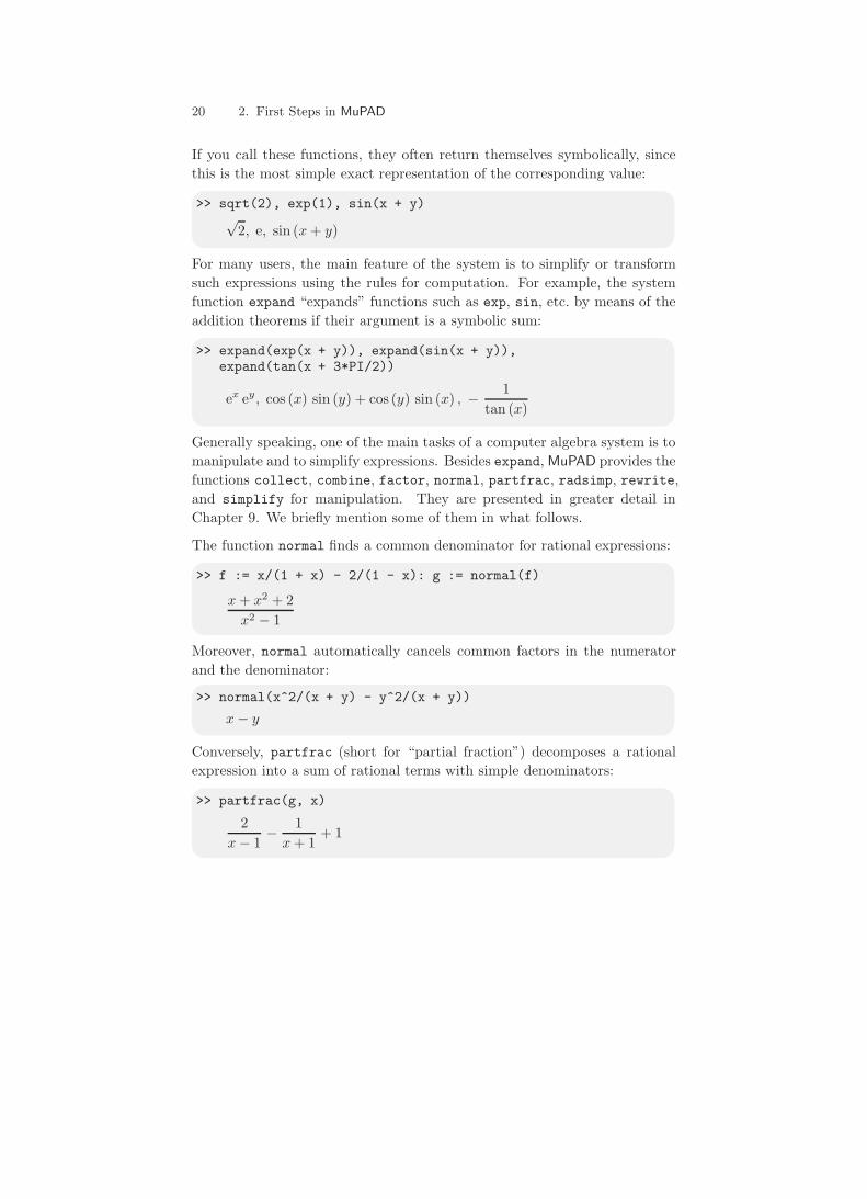
If you call these functions, they often return themselves symbolically, sincethis is the most simple exact representation of the corresponding value:

>> sqrt(2), exp(1), sin(x + y)√

2, e, sin (x + y)

For many users, the main feature of the system is to simplify or transformsuch expressions using the rules for computation. For example, the systemfunction expand “expands” functions such as exp, sin, etc. by means of theaddition theorems if their argument is a symbolic sum:

>> expand(exp(x + y)), expand(sin(x + y)),expand(tan(x + 3*PI/2))

ex ey, cos (x) sin (y) + cos (y) sin (x) , − 1tan (x)

Generally speaking, one of the main tasks of a computer algebra system is tomanipulate and to simplify expressions. Besides expand, MuPAD provides thefunctions collect, combine, factor, normal, partfrac, radsimp, rewrite,and simplify for manipulation. They are presented in greater detail inChapter 9. We briefly mention some of them in what follows.

The function normal finds a common denominator for rational expressions:

>> f := x/(1 + x) - 2/(1 - x): g := normal(f)

x + x2 + 2x2 − 1

Moreover, normal automatically cancels common factors in the numeratorand the denominator:

>> normal(x^2/(x + y) - y^2/(x + y))

x − y

Conversely, partfrac (short for “partial fraction”) decomposes a rationalexpression into a sum of rational terms with simple denominators:

>> partfrac(g, x)

2x − 1

− 1x + 1

+ 1


The function simplify is a universal simplifier and tries to find a represent-ation that is as simple as possible:

>> simplify((exp(x) - 1)/(exp(x/2) + 1))

ex2 − 1

You may control the simplification by supplying simplify with additionalarguments (see ?simplify). The function radsimp simplifies arithmeticalexpressions containing radicals (roots):

>> f := sqrt(4 + 2*sqrt(3)): f = radsimp(f)√√3 + 2

√2 =

√3 + 1

Here, we have generated an equation, which is a genuine MuPAD object.

Another important function is factor, which decomposes an expression intoa product of simpler ones:

>> factor(x^3 + 3*x^2 + 3*x + 1),factor(2*x*y - 2*x - 2*y + x^2 + y^2),factor(x^2/(x + y) - z^2/(x + y))

(x + 1)3 , (x + y − 2) · (x + y) ,(x − z) · (x + z)

(x + y)

The function limit does what its name suggests. For example, the functionsin(x)/x has a removable pole at x = 0. Its limit for x → 0 is 1:

>> limit(sin(x)/x, x = 0)

1

In a MuPAD session, you can define functions of your own in several ways.A simple and intuitive method is to use the arrow operator -> (the minussymbol followed by the “greater than” symbol):

>> F := x -> (x^2): F(x), F(y), F(a + b), F’(x)

x2, y2, (a + b)2 , 2 x

In Chapter 18, we discuss MuPAD’s programming features and describe howto implement more complex algorithms as MuPAD procedures.


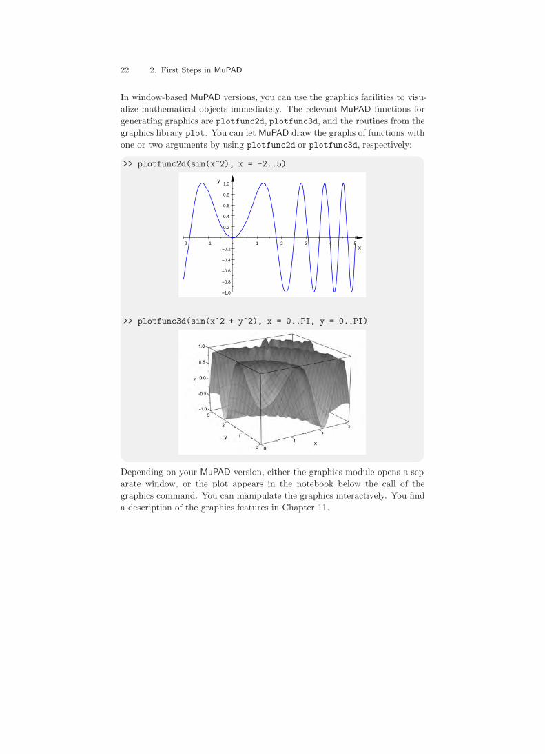
In window-based MuPAD versions, you can use the graphics facilities to visu-alize mathematical objects immediately. The relevant MuPAD functions forgenerating graphics are plotfunc2d, plotfunc3d, and the routines from thegraphics library plot. You can let MuPAD draw the graphs of functions withone or two arguments by using plotfunc2d or plotfunc3d, respectively:

>> plotfunc2d(sin(x^2), x = -2..5)

−2 −1 1 2 3 4 5

−1.0

−0.8

−0.6

−0.4

−0.2

0.2

0.4

0.6

0.8

1.0

x

y

>> plotfunc3d(sin(x^2 + y^2), x = 0..PI, y = 0..PI)

Depending on your MuPAD version, either the graphics module opens a sep-arate window, or the plot appears in the notebook below the call of thegraphics command. You can manipulate the graphics interactively. You finda description of the graphics features in Chapter 11.


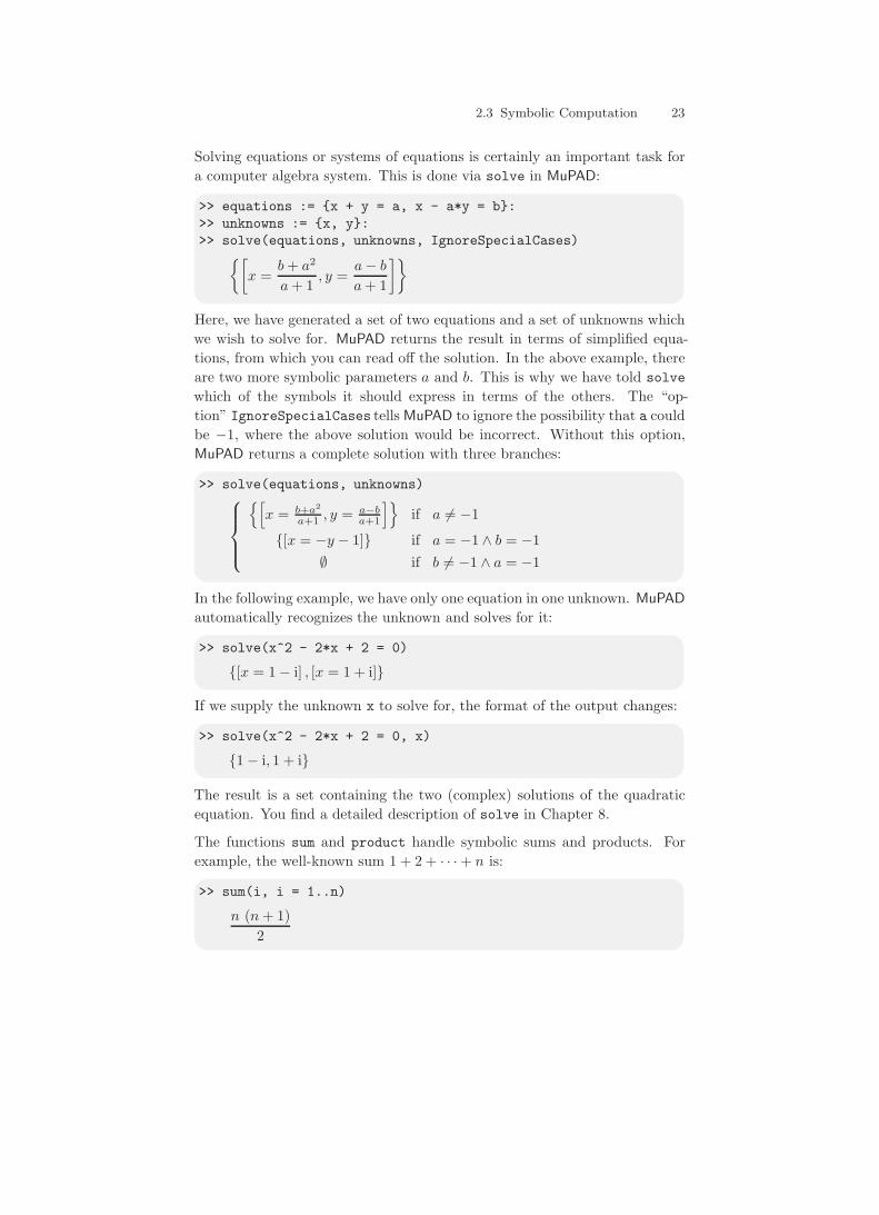
Solving equations or systems of equations is certainly an important task fora computer algebra system. This is done via solve in MuPAD:

>> equations := {x + y = a, x - a*y = b}:>> unknowns := {x, y}:>> solve(equations, unknowns, IgnoreSpecialCases){[

x =b + a2

a + 1, y =

a − b

a + 1

]}

Here, we have generated a set of two equations and a set of unknowns whichwe wish to solve for. MuPAD returns the result in terms of simplified equa-tions, from which you can read off the solution. In the above example, thereare two more symbolic parameters a and b. This is why we have told solvewhich of the symbols it should express in terms of the others. The “op-tion” IgnoreSpecialCases tells MuPAD to ignore the possibility that a couldbe −1, where the above solution would be incorrect. Without this option,MuPAD returns a complete solution with three branches:

>> solve(equations, unknowns)⎧⎪⎪⎨⎪⎪⎩

{[x = b+a2

a+1 , y = a−ba+1

]}if a �= −1

{[x = −y − 1]} if a = −1 ∧ b = −1∅ if b �= −1 ∧ a = −1

In the following example, we have only one equation in one unknown. MuPADautomatically recognizes the unknown and solves for it:

>> solve(x^2 - 2*x + 2 = 0)

{[x = 1 − i] , [x = 1 + i]}

If we supply the unknown x to solve for, the format of the output changes:

>> solve(x^2 - 2*x + 2 = 0, x)

{1 − i, 1 + i}

The result is a set containing the two (complex) solutions of the quadraticequation. You find a detailed description of solve in Chapter 8.

The functions sum and product handle symbolic sums and products. Forexample, the well-known sum 1 + 2 + · · · + n is:

>> sum(i, i = 1..n)

n (n + 1)2


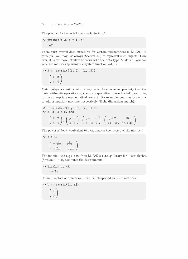
The product 1 · 2 · · ·n is known as factorial n!:

>> product(i^3, i = 1..n)

n!3

There exist several data structures for vectors and matrices in MuPAD. Inprinciple, you may use arrays (Section 4.9) to represent such objects. How-ever, it is far more intuitive to work with the data type “matrix.” You cangenerate matrices by using the system function matrix:

>> A := matrix([[1, 2], [a, 4]])(1 2a 4

)

Matrix objects constructed this way have the convenient property that thebasic arithmetic operations +, *, etc. are specialized (“overloaded”) accordingto the appropriate mathematical context. For example, you may use + or *to add or multiply matrices, respectively (if the dimensions match):

>> B := matrix([[y, 3], [z, 5]]):>> A, B, A + B, A*B(

1 2a 4

),

(y 3z 5

),

(y + 1 5a + z 9

),

(y + 2 z 13

4 z + a y 3 a + 20

)

The power A^(-1), equivalent to 1/A, denotes the inverse of the matrix:

>> A^(-1)(− 2

a−21

a−2a

2 a−4 − 12 a−4

)

The function linalg::det, from MuPAD’s linalg library for linear algebra(Section 4.15.4), computes the determinant:

>> linalg::det(A)

4 − 2 a

Column vectors of dimension n can be interpreted as n × 1 matrices:

>> b := matrix([1, x])(1x

)


You can comfortably determine the solution A−1b of the system of linearequations Ax = b, with the above coefficient matrix A and the previouslydefined b on the right hand side:

>> solutionVector := A^(-1)*b(x

a−2 − 2a−2

a2 a−4 − x

2 a−4

)

Now you can apply the function normal to each component of the vector bymeans of the system function map, thus simplifying the representation:

>> map(%, normal)(x−2a−2a−x2 a−4

)

To verify MuPAD’s computation, you may multiply the solution vector bythe matrix A:

>> A * %(2 (a−x)2 a−4 + x−2

a−24 (a−x)2 a−4 + a (x−2)

a−2

)

After simplification, you can check that the result equals b:

>> map(%, normal)(1x

)

Section 4.15 provides more information on handling matrices and vectors.

Exercise 2.3: Compute an expanded form of the expression (x2 + y)5.

Exercise 2.4: Use MuPAD to check thatx2 − 1x + 1

= x − 1 holds.

Exercise 2.5: Generate a plot of the function 1/ sin(x) for 1 ≤ x ≤ 10 .


Exercise 2.6: Obtain detailed information about the function limit. UseMuPAD to verify the following limits:

limx→0

sin(x)x

= 1 , limx→0

1 − cos(x)x

= 0 , limx→0+

ln(x) = −∞ ,

limx→0

xsin(x) = 1 , limx→∞

(1 +

1x

)x

= e , limx→∞

ln(x)ex

= 0 ,

limx→0+

xln(x) = ∞ , limx→∞

(1 +

π

x

)x

= eπ , limx→0−

21 + e−1/x

= 0 .

The limit limx→0

ecot(x) does not exist. How does MuPAD react?

Exercise 2.7: Obtain detailed information about the function sum. The callsum(f(k),k = a..b) computes a closed form of a finite or infinite sum, ifpossible. Use MuPAD to verify the following identity:

n∑k=1

(k2 + k + 1) =n (n2 + 3 n + 5)

3.

Determine the values of the following series:

∞∑k=0

2 k − 3(k + 1) (k + 2) (k + 3)

,

∞∑k=2

k

(k − 1)2 (k + 1)2.

Exercise 2.8: Compute 2 · (A + B), A · B, and (A − B)−1 for the followingmatrices:

A =

⎛⎝ 1 2 3

4 5 67 8 0

⎞⎠ , B =

⎛⎝ 1 1 0

0 0 10 1 0

⎞⎠ .

2.3.2 Curve Sketching

In the following sample session, we use some of the system functions fromthe previous section to sketch and discuss the curve given by the rationalfunction

f : x �→ (x − 1)2

x − 2+ a

with a parameter a. First, we determine some characteristics of this function:discontinuities, extremal values, and behavior for large x.


>> f := x -> ((x - 1)^2/(x - 2) + a):>> singularities := discont(f(x), x)

{2}

The function discont determines the discontinuities of the function f withrespect to the variable x. It returns a set of such points. Thus, the above f

is defined and continuous for all x �= 2. Obviously, x = 2 is a pole. Indeed,MuPAD finds the limit ∓∞ when you approach this point from the left orfrom the right, respectively:

>> limit(f(x), x = 2, Left), limit(f(x), x = 2, Right)

−∞, ∞

You find the roots of f by solving the equation f = 0:

>> roots := solve(f(x) = 0, x){1 −

√a (a + 4)

2− a

2,

√a (a + 4)

2− a

2+ 1

}

Depending on a, either both or none of the two roots are real. Now, we wantto find the local extrema of f . To this end, we determine the roots of thefirst derivative f ′:

>> f’(x)

2 x − 2x − 2

− (x − 1)2

(x − 2)2

>> extrema := solve(f’(x) = 0, x)

{1, 3}

These are the candidates for local extrema. However, some of them mightbe saddle points. If the second derivative f ′′ does not vanish at these points,then both are really extrema. We check:

>> f’’(1), f’’(3)

−2, 2

Our results imply that f has the following properties: for any choice of theparameter a, there is a local maximum at x = 1, a pole at x = 2, and a localminimum at x = 3. The corresponding values of f at these points are


>> maxvalue := f(1); minvalue := f(3)a

a + 4

f tends to ∓∞ for x → ∓∞:

>> limit(f(x), x = -infinity), limit(f(x), x = infinity)

−∞, ∞

We can specify the behavior of f more precisely for large values of x. Itasymptotically approaches the linear function x �→ x + a:

>> series(f(x), x = infinity)

x + a +1x

+2x2

+4x3

+8x4

+ O

(1x5

)

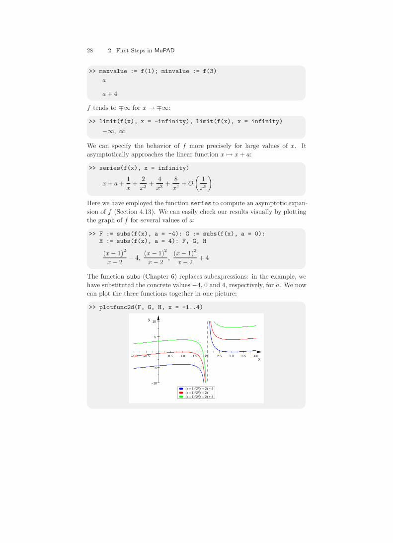
Here we have employed the function series to compute an asymptotic expan-sion of f (Section 4.13). We can easily check our results visually by plottingthe graph of f for several values of a:

>> F := subs(f(x), a = -4): G := subs(f(x), a = 0):H := subs(f(x), a = 4): F, G, H

(x − 1)2

x − 2− 4,

(x − 1)2

x − 2,

(x − 1)2

x − 2+ 4

The function subs (Chapter 6) replaces subexpressions: in the example, wehave substituted the concrete values −4, 0 and 4, respectively, for a. We nowcan plot the three functions together in one picture:

>> plotfunc2d(F, G, H, x = -1..4)

(x − 1)^2/(x − 2) − 4(x − 1)^2/(x − 2)(x − 1)^2/(x − 2) + 4

−1.0 −0.5 0.5 1.0 1.5 2.0 2.5 3.0 3.5 4.0

−10

−5

5

10

x

y


2.3.3 Elementary Number Theory

MuPAD provides a lot of elementary number theoretic functions, for example:

• isprime(n) tests whether n ∈ N is a prime number,

• ithprime(n) returns the n-th prime number,

• nextprime(n) finds the least prime number ≥ n,

• ifactor(n) computes the prime factorization of n.

These routines are quite fast. However, since they employ probabilistic prim-ality tests, they may return wrong results with very small probability.6 In-stead of isprime, you can use the (slower) function numlib::proveprime asan error-free primality test.

Let us generate a list of all primes up to 10 000. Here is one of many ways todo this:

>> primes := select([$ 1..10000], isprime)[2, 3, 5, 7, 11, 13, 17, ..., 9949, 9967, 9973]

First, we have generated the sequence of all positive integers up to 10 000by means of the sequence generator $ (Section 4.5). The square brackets [ ]convert this to a MuPAD list. Then select (Section 4.6) eliminates all thoselist elements for which the function isprime, supplied as second argument,returns FALSE. The number of these primes equals the number of list elements,which we can obtain via nops (“number of operands,” Section 4.1):

>> nops(primes)

1229

Alternatively, we may generate the same prime list by

>> primes := [ithprime(i) $ i = 1..1229]:

Here we have used the fact that we already know the number of primes up to10 000. Another possibility is to generate a large list of primes and discardthe ones greater than 10 000:

>> primes := select([ithprime(i) $ i=1..5000],x -> (x<=10000)):

6 In practice, you need not worry about this because the chances of a wronganswer are negligible: the probability of a hardware failure is much higher thanthe probability that the randomized test returns the wrong answer on a correctlyworking hardware.


Here, the object x -> (x <= 10000) represents the function that maps each xto the inequality x <= 10000. The select command then keeps only thoselist elements for which the inequality evaluates to TRUE.

In the next example, we use a repeat loop (Chapter 16) to generate the listof primes. With the help of the concatenation operator . (Section 4.6), wesuccessively append primes i to a list until nextprime(i+1), the next primegreater than i, exceeds 10 000. We start with the empty list and the firstprime i = 2:

>> primes := []: i := 2:>> repeat

primes := primes . [i];i := nextprime(i + 1)

until i > 10000 end_repeat:

Now, we consider Goldbach’s famous conjecture:

“Every even integer greater than 2 is the sum of two primes.”

We want to verify this conjecture for all even numbers up to 10 000. First,we generate the list of even integers [4, 6, . . . , 10000]:

>> list := [2*i $ i = 2..5000]:>> nops(list)

4999

Now, we select those numbers from the list that cannot be written in theform “prime + 2.” This is done by testing for each i in the list whether i− 2is a prime:

>> list := select(list, i -> (not isprime(i - 2))):>> nops(list)

4998

The only integer that has been eliminated is 4 (since for all other even positiveintegers i−2 is even and greater than 2, and hence not prime). Now we discardall numbers of the form “prime + 3”:

>> list := select(list, i -> (not isprime(i - 3))):>> nops(list)

3770

The remaining 3770 integers are neither of the form “prime + 2” nor of theform “prime + 3.” We now continue this procedure by means of a whileloop (Chapter 16). In the loop, j successively runs through all primes > 3,


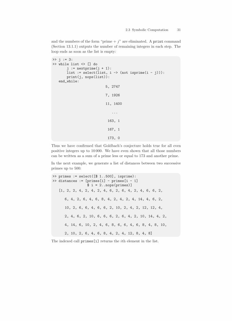
and the numbers of the form “prime + j” are eliminated. A print command(Section 13.1.1) outputs the number of remaining integers in each step. Theloop ends as soon as the list is empty:

>> j := 3:>> while list <> [] do

j := nextprime(j + 1):list := select(list, i -> (not isprime(i - j))):print(j, nops(list)):

end_while:5, 2747

7, 1926

11, 1400

...

163, 1

167, 1

173, 0

Thus we have confirmed that Goldbach’s conjecture holds true for all evenpositive integers up to 10 000. We have even shown that all those numberscan be written as a sum of a prime less or equal to 173 and another prime.

In the next example, we generate a list of distances between two successiveprimes up to 500:

>> primes := select([$ 1..500], isprime):>> distances := [primes[i] - primes[i - 1]

$ i = 2..nops(primes)][1, 2, 2, 4, 2, 4, 2, 4, 6, 2, 6, 4, 2, 4, 6, 6, 2,

6, 4, 2, 6, 4, 6, 8, 4, 2, 4, 2, 4, 14, 4, 6, 2,

10, 2, 6, 6, 4, 6, 6, 2, 10, 2, 4, 2, 12, 12, 4,

2, 4, 6, 2, 10, 6, 6, 6, 2, 6, 4, 2, 10, 14, 4, 2,

4, 14, 6, 10, 2, 4, 6, 8, 6, 6, 4, 6, 8, 4, 8, 10,

2, 10, 2, 6, 4, 6, 8, 4, 2, 4, 12, 8, 4, 8]

The indexed call primes[i] returns the ith element in the list.


The function zip (Section 4.6) provides an alternative method. The callzip(a, b, f) combines two lists a = [a1, a2, . . . ] and b = [b1, b2, . . . ] compon-entwise by means of the function f : the resulting list is

[f(a1, b1), f(a2, b2), . . . ]

and has as many elements as the shorter of the two lists. In our example,we apply this to the prime list a = [a1, . . . , an], the “shifted” prime listb = [a2, . . . , an], and the function (x, y) �→ y − x. We first generate a shiftedcopy of the prime list by deleting the first element, thus shortening the list:

>> b := primes: delete b[1]:

The following command returns the same result as above:

>> distances := zip(primes, b, (x, y) -> (y - x)):

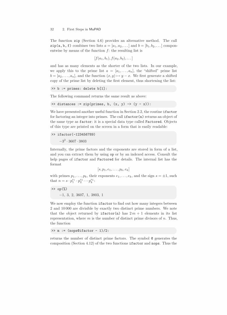
We have presented another useful function in Section 2.2, the routine ifactorfor factoring an integer into primes. The call ifactor(n) returns an object ofthe same type as factor: it is a special data type called Factored. Objectsof this type are printed on the screen in a form that is easily readable:

>> ifactor(-123456789)

−32 · 3607 · 3803

Internally, the prime factors and the exponents are stored in form of a list,and you can extract them by using op or by an indexed access. Consult thehelp pages of ifactor and Factored for details. The internal list has theformat

[s, p1, e1, . . . , pk, ek]

with primes p1, . . . , pk, their exponents e1, . . . , ek, and the sign s = ±1, suchthat n = s · pe1

1 · pe22 · · · pek

k :

>> op(%)

−1, 3, 2, 3607, 1, 3803, 1

We now employ the function ifactor to find out how many integers between2 and 10 000 are divisible by exactly two distinct prime numbers. We notethat the object returned by ifactor(n) has 2 m + 1 elements in its listrepresentation, where m is the number of distinct prime divisors of n. Thus,the function

>> m := (nops@ifactor - 1)/2:

returns the number of distinct prime factors. The symbol @ generates thecomposition (Section 4.12) of the two functions ifactor and nops. Thus the


call m(k) returns m(k) = (nops(ifactor(k))- 1)/2 for k being an integer.We construct the list of values m(k) for k = 2, . . . , 10000:

>> list := [m(k) $ k = 2..10000]:

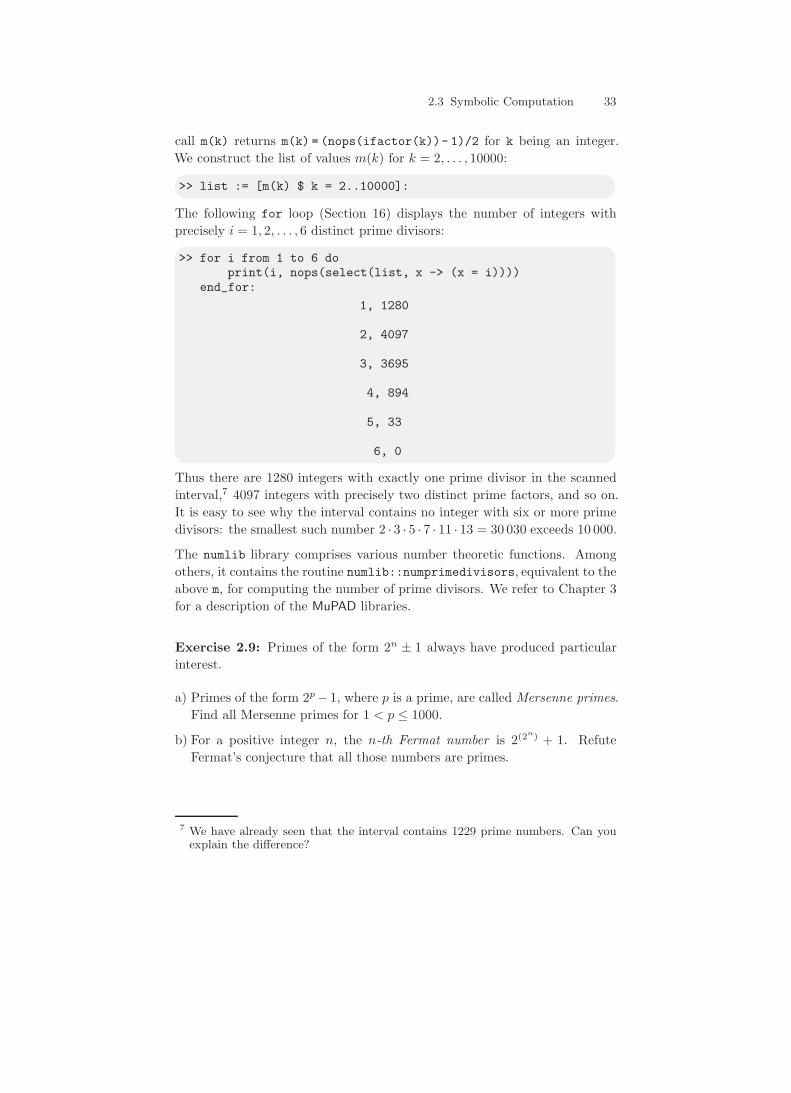
The following for loop (Section 16) displays the number of integers withprecisely i = 1, 2, . . . , 6 distinct prime divisors:

>> for i from 1 to 6 doprint(i, nops(select(list, x -> (x = i))))

end_for:1, 1280

2, 4097

3, 3695

4, 894

5, 33

6, 0

Thus there are 1280 integers with exactly one prime divisor in the scannedinterval,7 4097 integers with precisely two distinct prime factors, and so on.It is easy to see why the interval contains no integer with six or more primedivisors: the smallest such number 2 · 3 · 5 · 7 · 11 · 13 = 30 030 exceeds 10 000.

The numlib library comprises various number theoretic functions. Amongothers, it contains the routine numlib::numprimedivisors, equivalent to theabove m, for computing the number of prime divisors. We refer to Chapter 3for a description of the MuPAD libraries.

Exercise 2.9: Primes of the form 2n ± 1 always have produced particularinterest.

a) Primes of the form 2p − 1, where p is a prime, are called Mersenne primes.Find all Mersenne primes for 1 < p ≤ 1000.

b) For a positive integer n, the n-th Fermat number is 2(2n) + 1. RefuteFermat’s conjecture that all those numbers are primes.

7 We have already seen that the interval contains 1229 prime numbers. Can youexplain the difference?

2. first steps in mupad - buecher.de · 2. first steps in mupad computer algebra systems such as...

Documents