2. basics - ethz · 2. basics • data sources • ... • stock market (300 mio. transactions per...
TRANSCRIPT
Visualization, Summer Term 2002 20.05.2003
1
Visualization, Summer Term 03 VIS, University of Stuttgart1
2. Basics
• Data sources• Visualization pipeline• Data representation
• Domain• Data structures• Data values• Data classification
Visualization, Summer Term 03 VIS, University of Stuttgart2
2.1. Data Sources
• The capability of traditional presentation techniques is not sufficient for the increasing amount of data to be interpreted
• Data might come from any source with almost arbitrary size• Techniques to efficiently visualize large-scale data sets and new data types need
to be developed
• Real world• Measurements and observation
• Theoretical world• Mathematical and technical models
• Artificial world• Data that is designed
Visualization, Summer Term 2002 20.05.2003
2
Visualization, Summer Term 03 VIS, University of Stuttgart3
TB
GB
MB
2.1. Data Sources
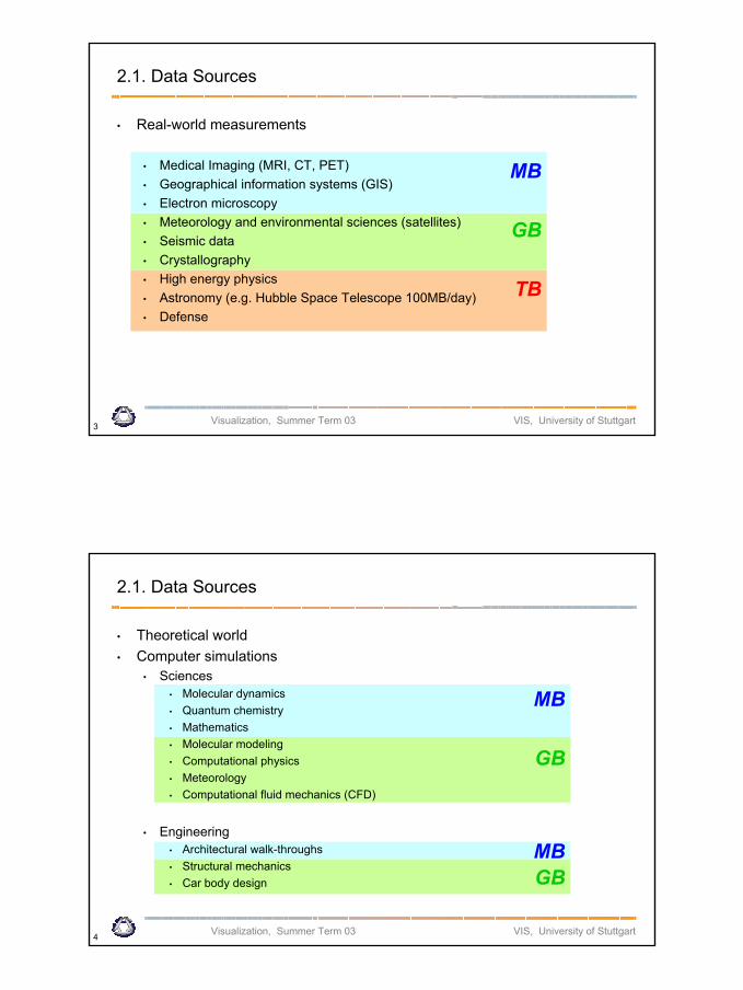
• Real-world measurements
• Medical Imaging (MRI, CT, PET)• Geographical information systems (GIS)• Electron microscopy• Meteorology and environmental sciences (satellites)• Seismic data• Crystallography• High energy physics• Astronomy (e.g. Hubble Space Telescope 100MB/day)• Defense
Visualization, Summer Term 03 VIS, University of Stuttgart4
MBGB
GB
MB
2.1. Data Sources
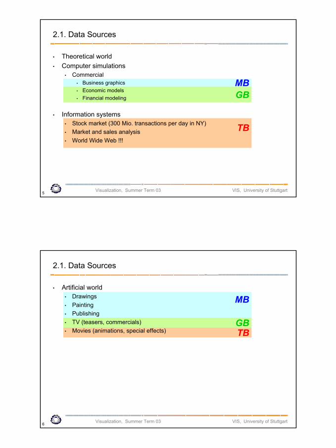
• Theoretical world• Computer simulations
• Sciences• Molecular dynamics• Quantum chemistry• Mathematics• Molecular modeling• Computational physics• Meteorology• Computational fluid mechanics (CFD)
• Engineering• Architectural walk-throughs• Structural mechanics• Car body design
Visualization, Summer Term 2002 20.05.2003
3
Visualization, Summer Term 03 VIS, University of Stuttgart5
TB
MBGB
2.1. Data Sources
• Theoretical world• Computer simulations
• Commercial • Business graphics• Economic models• Financial modeling
• Information systems• Stock market (300 Mio. transactions per day in NY)• Market and sales analysis• World Wide Web !!!
Visualization, Summer Term 03 VIS, University of Stuttgart6
TBGB
MB
2.1. Data Sources
• Artificial world• Drawings• Painting• Publishing• TV (teasers, commercials)• Movies (animations, special effects)
Visualization, Summer Term 2002 20.05.2003
4
Visualization, Summer Term 03 VIS, University of Stuttgart7
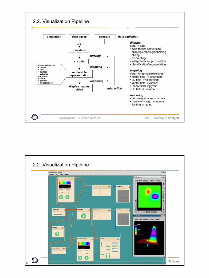
2.2. Visualization Pipeline
simulation data bases sensors
raw data
vis data
renderablerepresentation
display images video
graph. primitives:• points• lines• surface• volumesattributes:• color• texture• transparency
filtering
mapping
rendering
interaction
data aquisition
filteringdata -> data• data format conversion• clipping/cropping/denoising• slicing• resampling• interpolation/approximation• classification/segmentation
mappingdata ->graphical primitives• scalar field ->isosurface• 2D field ->height field• vector field ->vectors• tensor field ->glyphs• 3D field -> volume
rendering:• geometry/images/volumes• “realism“ – e.g. : shadows,
lighting, shading
Visualization, Summer Term 03 VIS, University of Stuttgart8
2.2. Visualization Pipeline
Visualization, Summer Term 2002 20.05.2003
5
Visualization, Summer Term 03 VIS, University of Stuttgart9
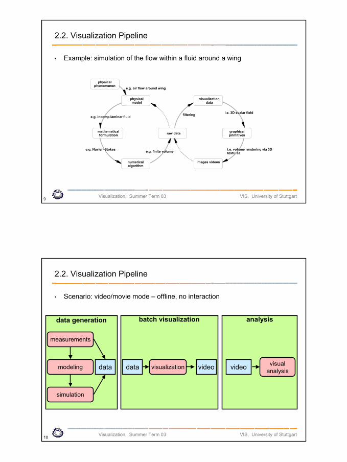
2.2. Visualization Pipeline
• Example: simulation of the flow within a fluid around a wing
i.e. volume rendering via 3D textures
physical phenomenon
physical model
mathematical formulation
numerical algorithm
images videos
graphical primitives
visualization data
e.g. air flow around wing
e.g. incomp.laminar fluid
e.g. Navier–Stokes e.g. finite volume
filtering i.e. 3D scalar field
raw data
Visualization, Summer Term 03 VIS, University of Stuttgart10
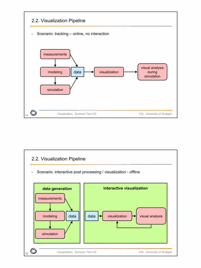
2.2. Visualization Pipeline
• Scenario: video/movie mode – offline, no interaction
data generation
measurements
modeling
simulation
data
batch visualization
visualizationdata video
analysis
video visualanalysis
Visualization, Summer Term 2002 20.05.2003
6
Visualization, Summer Term 03 VIS, University of Stuttgart11
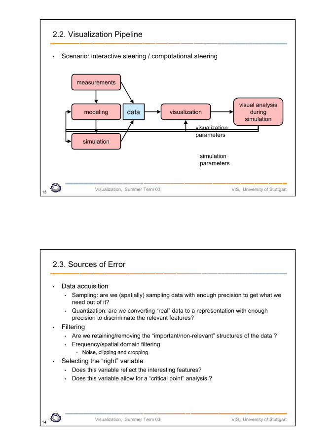
2.2. Visualization Pipeline
• Scenario: tracking – online, no interaction
measurements
modeling
simulation
data visualizationvisual analysis
duringsimulation
Visualization, Summer Term 03 VIS, University of Stuttgart12
2.2. Visualization Pipeline
• Scenario: interactive post processing / visualization - offline
data generation
measurements
modeling
simulation
data
interactive visualization
visualizationdata visual analysis
Visualization, Summer Term 2002 20.05.2003
7
Visualization, Summer Term 03 VIS, University of Stuttgart13
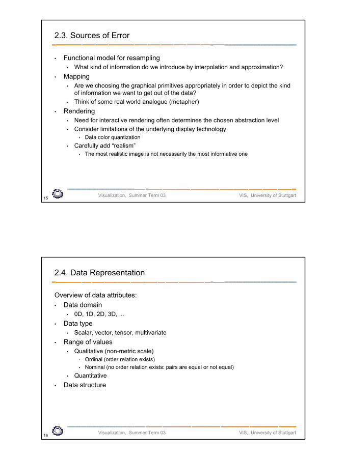
2.2. Visualization Pipeline
• Scenario: interactive steering / computational steering
measurements
modeling
simulation
data visualizationvisual analysis
duringsimulation
visualization parameters
simulation parameters
Visualization, Summer Term 03 VIS, University of Stuttgart14
2.3. Sources of Error
• Data acquisition• Sampling: are we (spatially) sampling data with enough precision to get what we
need out of it?• Quantization: are we converting “real” data to a representation with enough
precision to discriminate the relevant features?• Filtering
• Are we retaining/removing the “important/non-relevant” structures of the data ?• Frequency/spatial domain filtering
• Noise, clipping and cropping
• Selecting the “right” variable • Does this variable reflect the interesting features?• Does this variable allow for a “critical point” analysis ?
Visualization, Summer Term 2002 20.05.2003
8
Visualization, Summer Term 03 VIS, University of Stuttgart15
2.3. Sources of Error
• Functional model for resampling• What kind of information do we introduce by interpolation and approximation?
• Mapping• Are we choosing the graphical primitives appropriately in order to depict the kind
of information we want to get out of the data?• Think of some real world analogue (metapher)
• Rendering• Need for interactive rendering often determines the chosen abstraction level• Consider limitations of the underlying display technology
• Data color quantization• Carefully add “realism”
• The most realistic image is not necessarily the most informative one
Visualization, Summer Term 03 VIS, University of Stuttgart16
2.4. Data Representation
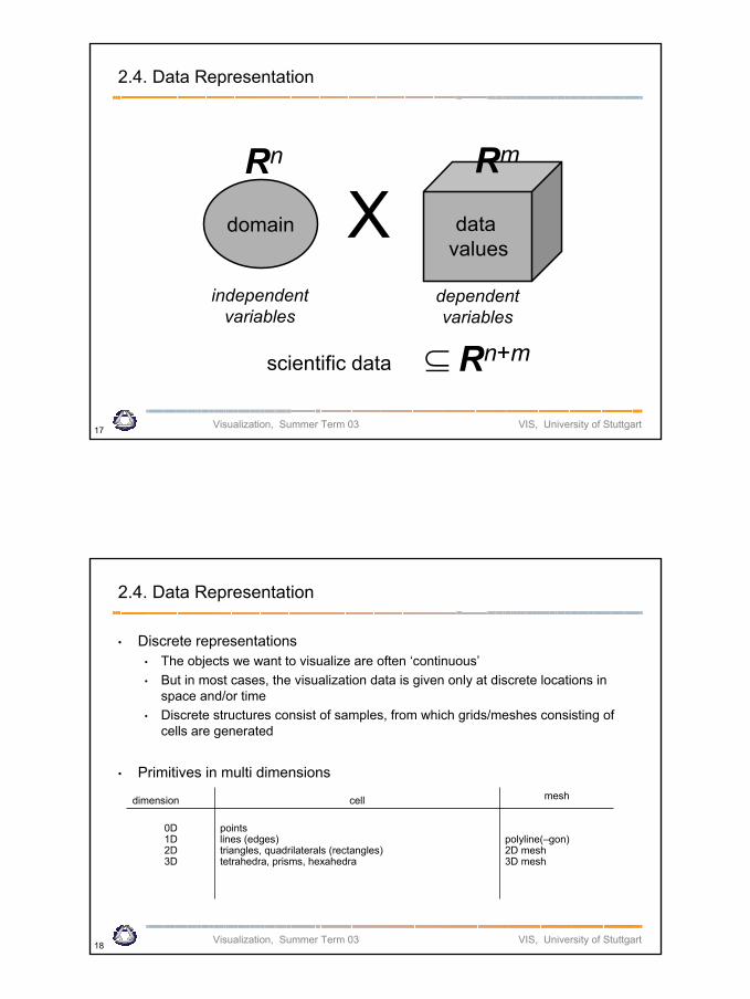
Overview of data attributes:• Data domain
• 0D, 1D, 2D, 3D, ...• Data type
• Scalar, vector, tensor, multivariate• Range of values
• Qualitative (non-metric scale)• Ordinal (order relation exists)• Nominal (no order relation exists: pairs are equal or not equal)
• Quantitative • Data structure
Visualization, Summer Term 2002 20.05.2003
9
Visualization, Summer Term 03 VIS, University of Stuttgart17
2.4. Data Representation
domain
independentvariables
Rn
data values
Xdependentvariables
Rm
scientific data ⊆ Rn+m
Visualization, Summer Term 03 VIS, University of Stuttgart18
2.4. Data Representation
• Discrete representations• The objects we want to visualize are often ‘continuous’• But in most cases, the visualization data is given only at discrete locations in
space and/or time• Discrete structures consist of samples, from which grids/meshes consisting of
cells are generated
• Primitives in multi dimensions
polyline(–gon)2D mesh3D mesh
pointslines (edges)triangles, quadrilaterals (rectangles)tetrahedra, prisms, hexahedra
0D1D2D3D
meshcelldimension
Visualization, Summer Term 2002 20.05.2003
10
Visualization, Summer Term 03 VIS, University of Stuttgart19
2.4. Data Representation
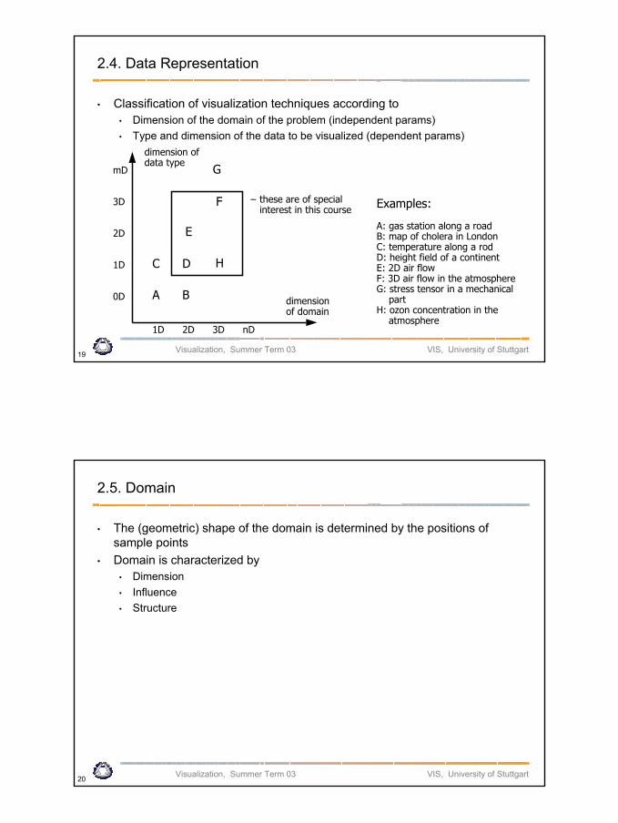
mD
3D
2D
1D
0D
1D 2D 3D nD
dimension of domain
G
C D
A B
F
E
H
– these are of special interest in this course Examples:
A: gas station along a roadB: map of cholera in LondonC: temperature along a rodD: height field of a continentE: 2D air flowF: 3D air flow in the atmosphereG: stress tensor in a mechanical
partH: ozon concentration in the
atmosphere
dimension of data type
• Classification of visualization techniques according to• Dimension of the domain of the problem (independent params)• Type and dimension of the data to be visualized (dependent params)
Visualization, Summer Term 03 VIS, University of Stuttgart20
2.5. Domain
• The (geometric) shape of the domain is determined by the positions of sample points
• Domain is characterized by• Dimension• Influence• Structure
Visualization, Summer Term 2002 20.05.2003
11
Visualization, Summer Term 03 VIS, University of Stuttgart21
2.5. Domain
• Influence of data points• Values at sample points influence the data distribution in a certain region around
these samples• To reconstruct the data at arbitrary points within the domain, the distribution of all
samples has to be calculated• Point influence
• Only influence on point itself• Local influence
• Only within a certain region• Voronoi-diagram• Cell-wise interpolation (see later in course)
• Global influence• Each sample might influence any other point within the domain
• Material properties for whole object• Scattered data interpolation
Visualization, Summer Term 03 VIS, University of Stuttgart22
2.5. Domain
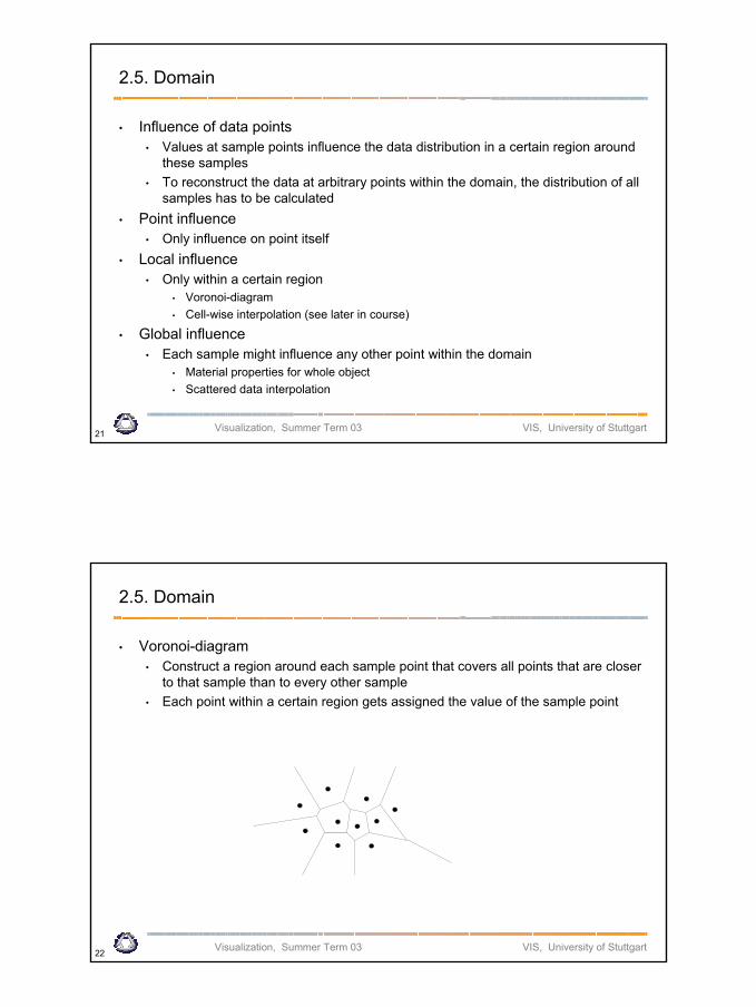
• Voronoi-diagram• Construct a region around each sample point that covers all points that are closer
to that sample than to every other sample• Each point within a certain region gets assigned the value of the sample point
Visualization, Summer Term 2002 20.05.2003
12
Visualization, Summer Term 03 VIS, University of Stuttgart23
2.5. Domain
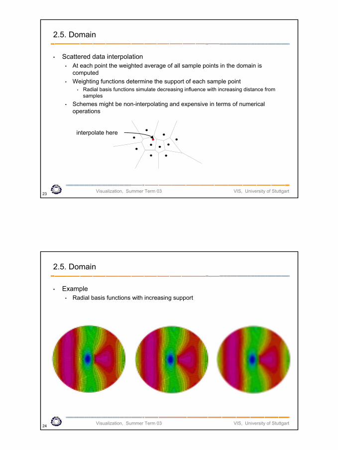
• Scattered data interpolation• At each point the weighted average of all sample points in the domain is
computed• Weighting functions determine the support of each sample point
• Radial basis functions simulate decreasing influence with increasing distance from samples
• Schemes might be non-interpolating and expensive in terms of numerical operations
interpolate here
Visualization, Summer Term 03 VIS, University of Stuttgart24
2.5. Domain
• Example • Radial basis functions with increasing support
Visualization, Summer Term 2002 20.05.2003
13
Visualization, Summer Term 03 VIS, University of Stuttgart25
2.6. Data Structures
• Requirements:• Convenience of access• Space efficiency• Lossless vs. lossy • Portability
• binary – less portable, more space/time efficient• text – human readable, portable, less space/time efficient
• Definition • If points are arbitrarily distributed and no connectivity exists between them, the
data is called scattered• Otherwise, the data is composed of cells bounded by grid lines• Topology specifies the structure (connectivity) of the data • Geometry specifies the position of the data
Visualization, Summer Term 03 VIS, University of Stuttgart26
2.6. Data Structures
• Some definitions concerning topology and geometry• In topology qualitative questions about geometrical structures are the main
concern. • Does it have any holes in it ?• Is it all connected together• Can it be separated into parts ?
• Underground map does not tell you how far one station is from the other, but rather how the lines are connected (topological map)
Visualization, Summer Term 2002 20.05.2003
14
Visualization, Summer Term 03 VIS, University of Stuttgart27
2.6. Data Structures
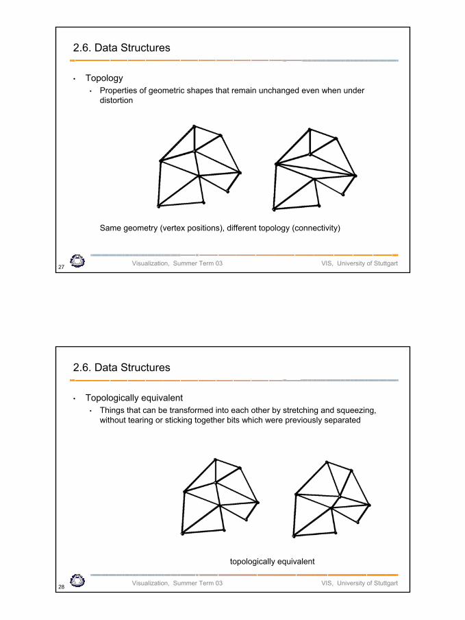
• Topology• Properties of geometric shapes that remain unchanged even when under
distortion
Same geometry (vertex positions), different topology (connectivity)
Visualization, Summer Term 03 VIS, University of Stuttgart28
2.6. Data Structures
• Topologically equivalent• Things that can be transformed into each other by stretching and squeezing,
without tearing or sticking together bits which were previously separated
topologically equivalent
Visualization, Summer Term 2002 20.05.2003
15
Visualization, Summer Term 03 VIS, University of Stuttgart29
2.6. Data Structures
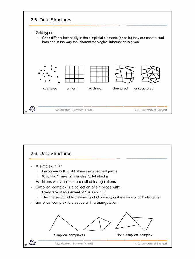
• Grid types• Grids differ substantially in the simplicial elements (or cells) they are constructed
from and in the way the inherent topological information is given
scattered uniform rectilinear structured unstructured
Visualization, Summer Term 03 VIS, University of Stuttgart30
2.6. Data Structures
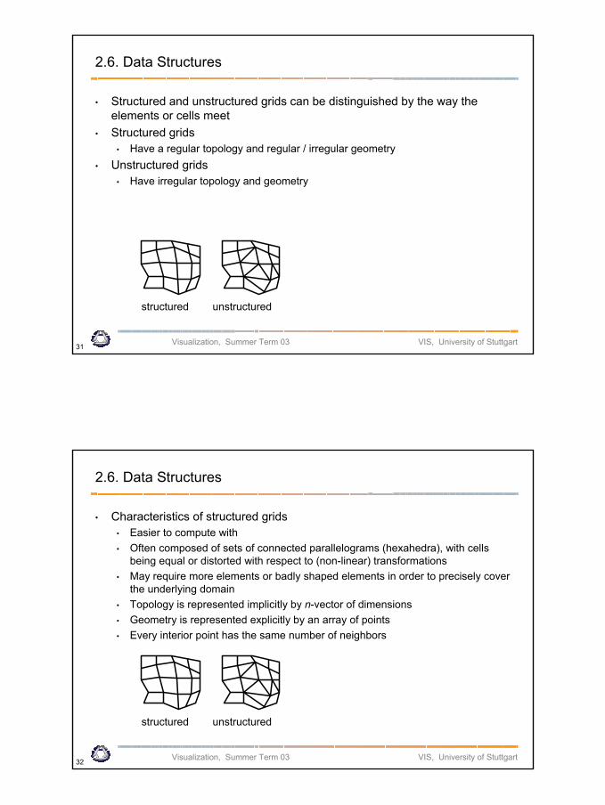
• A simplex in Rn
• the convex hull of n+1 affinely independent points• 0: points, 1: lines, 2: triangles, 3: tetrahedra
• Partitions via simplices are called triangulations• Simplical complex is a collection of simplices with:
• Every face of an element of C is also in C• The intersection of two elements of C is empty or it is a face of both elements
• Simplical complex is a space with a triangulation
Simplical complexes Not a simplical complex
Visualization, Summer Term 2002 20.05.2003
16
Visualization, Summer Term 03 VIS, University of Stuttgart31
2.6. Data Structures
• Structured and unstructured grids can be distinguished by the way the elements or cells meet
• Structured grids • Have a regular topology and regular / irregular geometry
• Unstructured grids• Have irregular topology and geometry
structured unstructured
Visualization, Summer Term 03 VIS, University of Stuttgart32
2.6. Data Structures
• Characteristics of structured grids• Easier to compute with• Often composed of sets of connected parallelograms (hexahedra), with cells
being equal or distorted with respect to (non-linear) transformations• May require more elements or badly shaped elements in order to precisely cover
the underlying domain• Topology is represented implicitly by n-vector of dimensions• Geometry is represented explicitly by an array of points• Every interior point has the same number of neighbors
structured unstructured
Visualization, Summer Term 2002 20.05.2003
17
Visualization, Summer Term 03 VIS, University of Stuttgart33
2.6. Data Structures
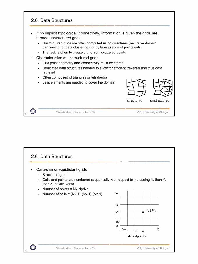
• If no implicit topological (connectivity) information is given the grids are termed unstructured grids
• Unstructured grids are often computed using quadtrees (recursive domain partitioning for data clustering), or by triangulation of points sets
• The task is often to create a grid from scattered points• Characteristics of unstructured grids
• Grid point geometry and connectivity must be stored• Dedicated data structures needed to allow for efficient traversal and thus data
retrieval• Often composed of triangles or tetrahedra• Less elements are needed to cover the domain
structured unstructured
Visualization, Summer Term 03 VIS, University of Stuttgart34
2.6. Data Structures
• Cartesian or equidistant grids• Structured grid• Cells and points are numbered sequentially with respect to increasing X, then Y,
then Z, or vice versa• Number of points = Nx•Ny•Nz• Number of cells = (Nx-1)•(Ny-1)•(Nz-1)
3
2
1
0
P[i,j,(k)]
dy
Y
3210dx
dx = dy = dz
X
Visualization, Summer Term 2002 20.05.2003
18
Visualization, Summer Term 03 VIS, University of Stuttgart35
2.6. Data Structures
• Cartesian grids• Vertex positions are given implicitly from [i,j,k]:
• P[i,j,k].x = origin + i • dx• P[i,j,k].y = origin + j • dy• P[i,j,k].z = origin + k • dz
• Global vertex index I[i,j,k] = k•Ny•Nx + j•Nx + i• k = l / (Ny•Nx)• j = (l % (Ny•Nx)) / Nx• i = (l % (Ny•Nx) % Nx)
• Global index allows for linear storage scheme• Wrong access pattern might destroy cache coherence
Visualization, Summer Term 03 VIS, University of Stuttgart36
2.6. Data Structures
• Uniform grids• Similar to Cartesian grids• Consist of equal cells but with different resolution in at least one dimension ( dx ≠
dy (≠ dz))• Spacing between grid points is constant in each dimension -> same indexing
scheme as for Cartesian grids• Most likely to occur in applications where the data is generated by a 3D imaging
device providing different sampling rates in each dimension• Typical example: medical volume data consisting of slice images
• Slice images with square pixels (dx = dy) • Larger slice distance (dz > dx = dy)
Visualization, Summer Term 2002 20.05.2003
19
Visualization, Summer Term 03 VIS, University of Stuttgart37
2.6. Data Structures
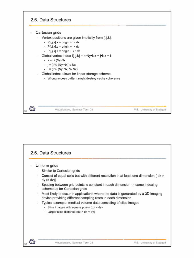
• Rectilinear grids• Topology is still regular but irregular spacing between grid points
• Non-linear scaling of positions along either axis• Spacing, x_coord[L], y_coord[M], z_coord[N], must be stored explicitly
• Topology is still implicit
M
Ni
j
Visualization, Summer Term 03 VIS, University of Stuttgart38
2.6. Data Structures
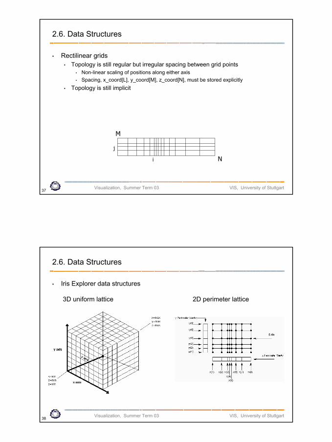
• Iris Explorer data structures
3D uniform lattice 2D perimeter lattice
Visualization, Summer Term 2002 20.05.2003
20
Visualization, Summer Term 03 VIS, University of Stuttgart39
2.6. Data Structures
• Curvilinear grids• Topology is still regular but irregular spacing between grid points
• Positions are non-linearly transformed• Topology is still implicit, but vertex positions are explicitly stored
• x_coord[L,M,N]• y_coord[L,M,N]• z_coord[L,M,N]
• Geometric structure might result in concave grids
Visualization, Summer Term 03 VIS, University of Stuttgart40
2.6. Data Structures
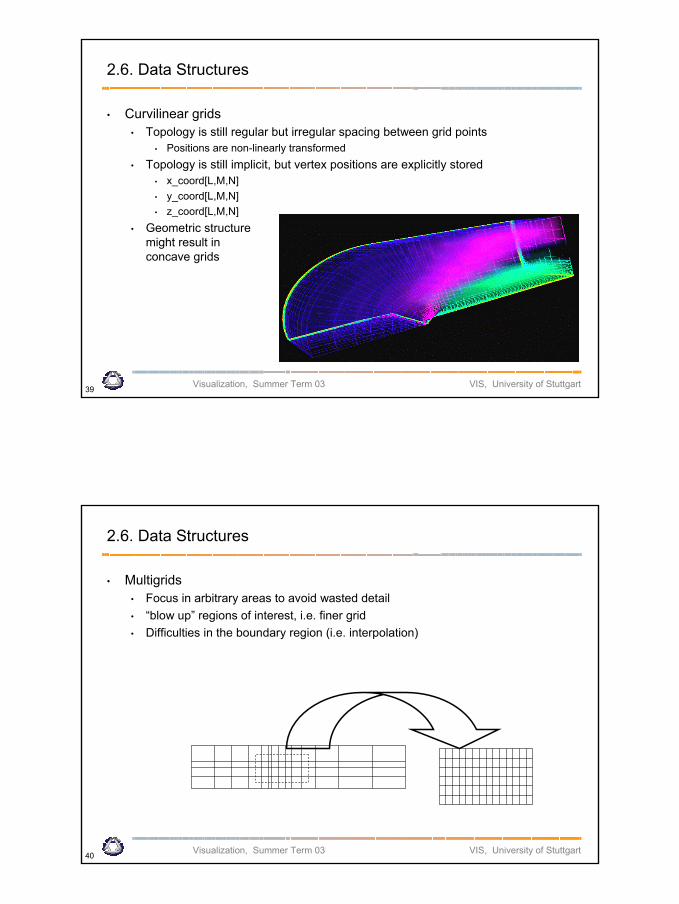
• Multigrids• Focus in arbitrary areas to avoid wasted detail• “blow up” regions of interest, i.e. finer grid• Difficulties in the boundary region (i.e. interpolation)
Visualization, Summer Term 2002 20.05.2003
21
Visualization, Summer Term 03 VIS, University of Stuttgart41
2.6. Data Structures
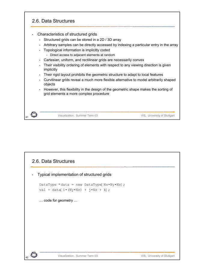
• Characteristics of structured grids• Structured grids can be stored in a 2D / 3D array• Arbitrary samples can be directly accessed by indexing a particular entry in the array• Topological information is implicitly coded
• Direct access to adjacent elements at random• Cartesian, uniform, and rectilinear grids are necessarily convex• Their visibility ordering of elements with respect to any viewing direction is given
implicitly• Their rigid layout prohibits the geometric structure to adapt to local features• Curvilinear grids reveal a much more flexible alternative to model arbitrarily shaped
objects• However, this flexibility in the design of the geometric shape makes the sorting of
grid elements a more complex procedure
Visualization, Summer Term 03 VIS, University of Stuttgart42
2.6. Data Structures
• Typical implementation of structured grids
DataType *data = new DataType[Nx•Ny•Nz];
val = data[i•(Ny•Nz) + j•Nz + k];
… code for geometry …
Visualization, Summer Term 2002 20.05.2003
22
Visualization, Summer Term 03 VIS, University of Stuttgart43
2.6. Data Structures
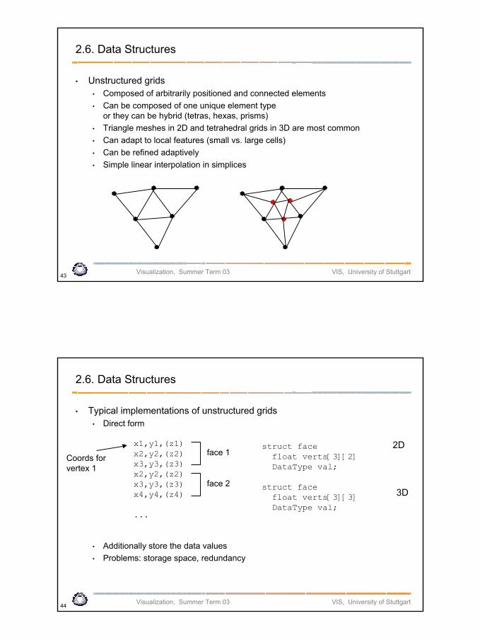
• Unstructured grids • Composed of arbitrarily positioned and connected elements• Can be composed of one unique element type
or they can be hybrid (tetras, hexas, prisms)• Triangle meshes in 2D and tetrahedral grids in 3D are most common• Can adapt to local features (small vs. large cells)• Can be refined adaptively• Simple linear interpolation in simplices
Visualization, Summer Term 03 VIS, University of Stuttgart44
2.6. Data Structures
• Typical implementations of unstructured grids• Direct form
• Additionally store the data values• Problems: storage space, redundancy
struct facefloat verts[3][2]DataType val;
struct facefloat verts[3][3]DataType val;
x1,y1,(z1) x2,y2,(z2)x3,y3,(z3)x2,y2,(z2) x3,y3,(z3)x4,y4,(z4)
...
face 1
face 2
2D
3D
Coords for vertex 1
Visualization, Summer Term 2002 20.05.2003
23
Visualization, Summer Term 03 VIS, University of Stuttgart45
2.6. Data Structures
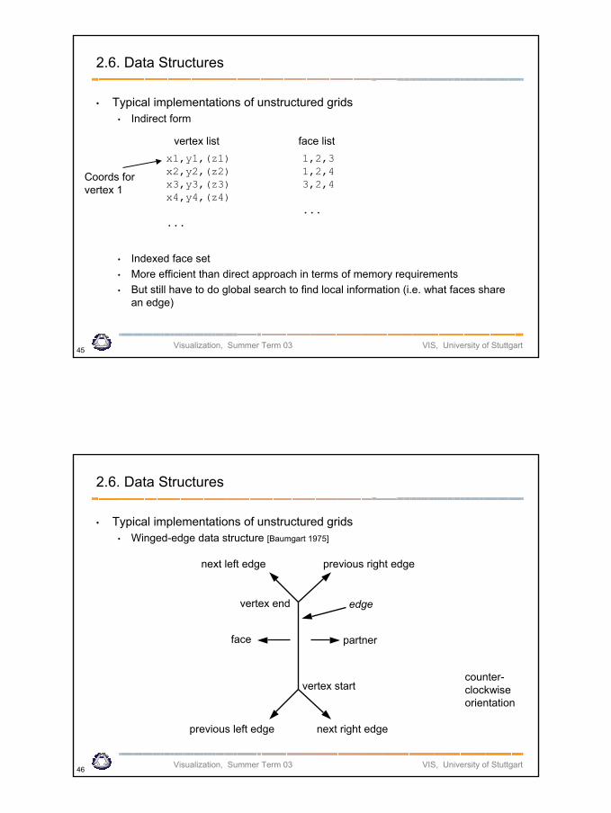
• Typical implementations of unstructured grids• Indirect form
• Indexed face set• More efficient than direct approach in terms of memory requirements• But still have to do global search to find local information (i.e. what faces share
an edge)
x1,y1,(z1) x2,y2,(z2)x3,y3,(z3)x4,y4,(z4)
...
vertex list face list1,2,3 1,2,43,2,4
...
Coords for vertex 1
Visualization, Summer Term 03 VIS, University of Stuttgart46
2.6. Data Structures
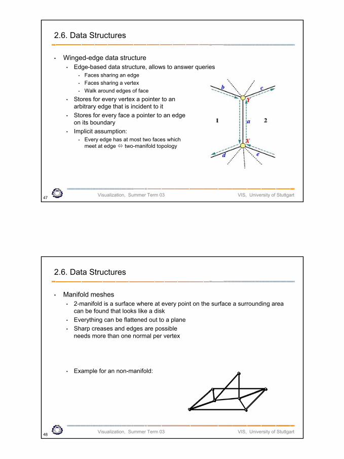
• Typical implementations of unstructured grids• Winged-edge data structure [Baumgart 1975]
next left edge previous right edge
edge
face partner
previous left edge next right edge
vertex start
vertex end
counter-clockwiseorientation
Visualization, Summer Term 2002 20.05.2003
24
Visualization, Summer Term 03 VIS, University of Stuttgart47
2.6. Data Structures
• Winged-edge data structure• Edge-based data structure, allows to answer queries
• Faces sharing an edge• Faces sharing a vertex• Walk around edges of face
• Stores for every vertex a pointer to anarbitrary edge that is incident to it
• Stores for every face a pointer to an edgeon its boundary
• Implicit assumption:• Every edge has at most two faces which
meet at edge two-manifold topology
Visualization, Summer Term 03 VIS, University of Stuttgart48
2.6. Data Structures
• Manifold meshes• 2-manifold is a surface where at every point on the surface a surrounding area
can be found that looks like a disk• Everything can be flattened out to a plane• Sharp creases and edges are possible
needs more than one normal per vertex
• Example for an non-manifold:
Visualization, Summer Term 2002 20.05.2003
25
Visualization, Summer Term 03 VIS, University of Stuttgart49
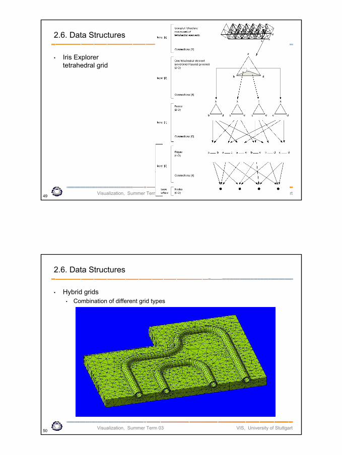
2.6. Data Structures
• Iris Explorertetrahedral grid
Visualization, Summer Term 03 VIS, University of Stuttgart50
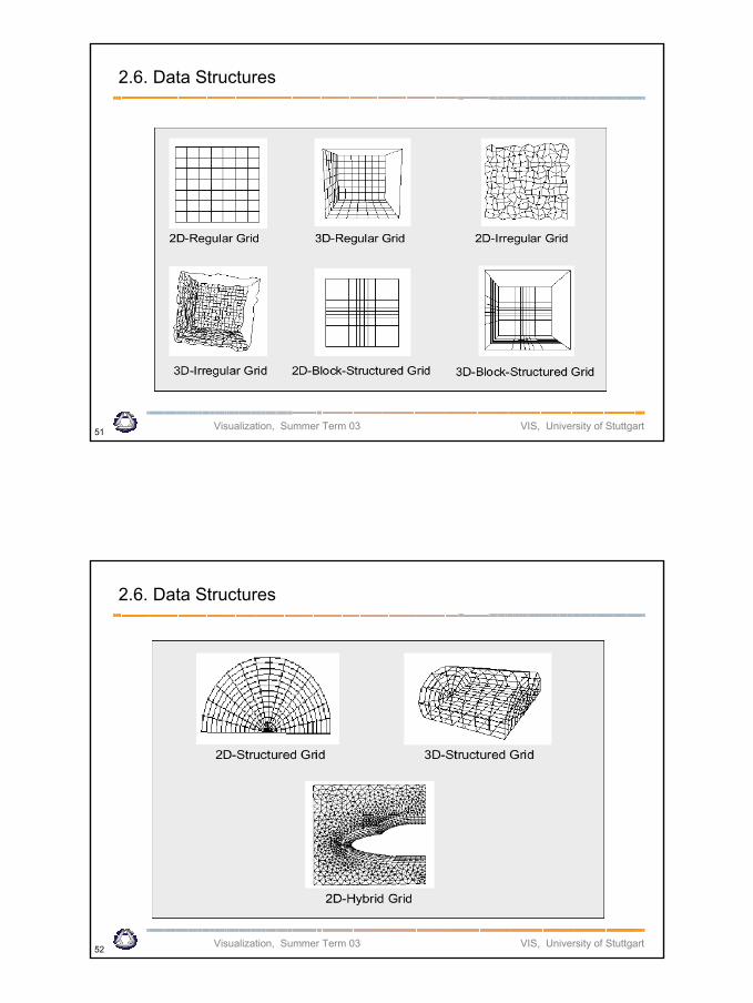
2.6. Data Structures
• Hybrid grids• Combination of different grid types
Visualization, Summer Term 2002 20.05.2003
26
Visualization, Summer Term 03 VIS, University of Stuttgart51
2.6. Data Structures
Visualization, Summer Term 03 VIS, University of Stuttgart52
2.6. Data Structures
Visualization, Summer Term 2002 20.05.2003
27
Visualization, Summer Term 03 VIS, University of Stuttgart53
2.6. Data Structures
Visualization, Summer Term 03 VIS, University of Stuttgart54
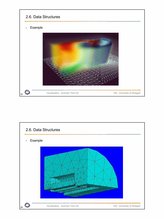
2.6. Data Structures
• Example
Visualization, Summer Term 2002 20.05.2003
28
Visualization, Summer Term 03 VIS, University of Stuttgart55
2.6. Data Structures
• Example
Visualization, Summer Term 03 VIS, University of Stuttgart56
2.6. Data Structures
• Example
Visualization, Summer Term 2002 20.05.2003
29
Visualization, Summer Term 03 VIS, University of Stuttgart57
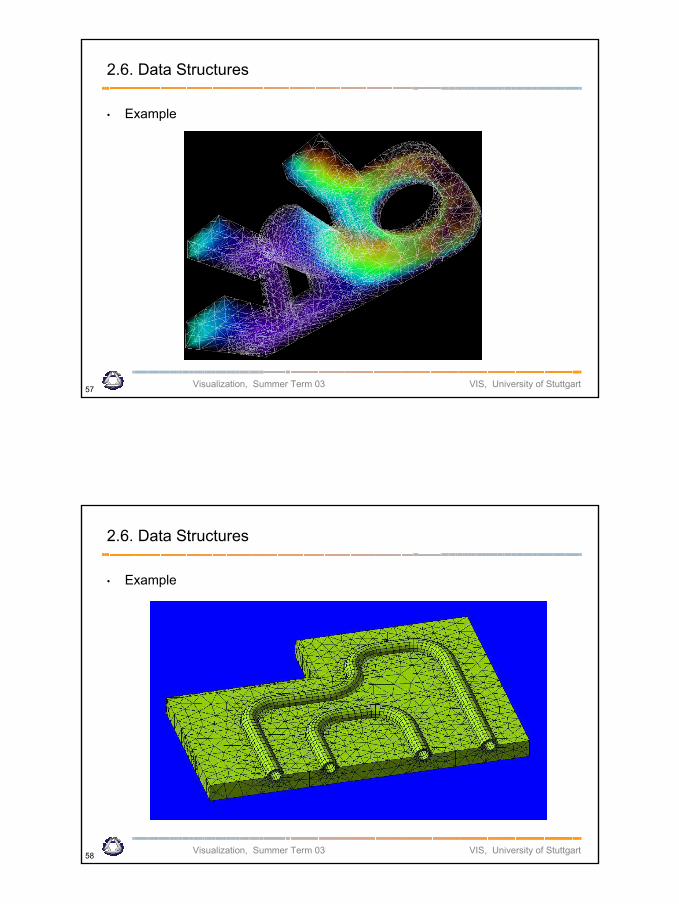
2.6. Data Structures
• Example
Visualization, Summer Term 03 VIS, University of Stuttgart58
2.6. Data Structures
• Example
Visualization, Summer Term 2002 20.05.2003
30
Visualization, Summer Term 03 VIS, University of Stuttgart59
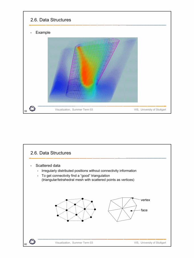
2.6. Data Structures
• Example
Visualization, Summer Term 03 VIS, University of Stuttgart60
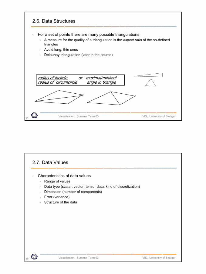
2.6. Data Structures
• Scattered data• Irregularly distributed positions without connectivity information• To get connectivity find a “good” triangulation
(triangular/tetrahedral mesh with scattered points as vertices)
vertex
face
Visualization, Summer Term 2002 20.05.2003
31
Visualization, Summer Term 03 VIS, University of Stuttgart61
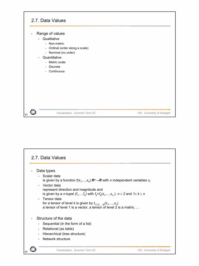
2.6. Data Structures
• For a set of points there are many possible triangulations• A measure for the quality of a triangulation is the aspect ratio of the so-defined
triangles• Avoid long, thin ones• Delaunay triangulation (later in the course)
radius of incircle or maximal/minimalradius of circumcircle angle in triangle
Visualization, Summer Term 03 VIS, University of Stuttgart62
2.7. Data Values
• Characteristics of data values• Range of values • Data type (scalar, vector, tensor data; kind of discretization)• Dimension (number of components)• Error (variance)• Structure of the data
Visualization, Summer Term 2002 20.05.2003
32
Visualization, Summer Term 03 VIS, University of Stuttgart63
2.7. Data Values
• Range of values • Qualitative
• Non-metric• Ordinal (order along a scale)• Nominal (no order)
• Quantitative• Metric scale• Discrete• Continuous
Visualization, Summer Term 03 VIS, University of Stuttgart64
2.7. Data Values
• Data types• Scalar data
is given by a function f(x1,...,xn):Rn→R with n independent variables xi
• Vector datarepresent direction and magnitude and is given by a n-tupel (f1,...,fn) with fk=fk(x1,...,xn ), n ≥ 2 and 1≤ k ≤ n
• Tensor datafor a tensor of level k is given by ti1,i2,…,ik(x1,…,xn)a tensor of level 1 is a vector, a tensor of level 2 is a matrix, …
• Structure of the data• Sequential (in the form of a list)• Relational (as table)• Hierarchical (tree structure)• Network structure
Visualization, Summer Term 2002 20.05.2003
33
Visualization, Summer Term 03 VIS, University of Stuttgart65
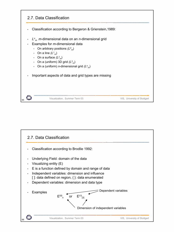
2.7. Data Classification
• Classification according to Bergeron & Grienstein,1989:
• Lnm m-dimensional data on an n-dimensional grid
• Examples for m-dimensional data • On arbitrary positions (L0
m)• On a line (L1
m)• On a surface (L2
m)• On a (uniform) 3D grid (L3
m)• On a (uniform) n-dimensional grid (Ln
m)
• Important aspects of data and grid types are missing
Visualization, Summer Term 03 VIS, University of Stuttgart66
2.7. Data Classification
• Classification according to Brodlie 1992:
• Underlying Field: domain of the data• Visualizing entity (E)• E is a function defined by domain and range of data• Independent variables: dimension and influence
[ ]: data defined on region, { }: data enumerated• Dependent variables: dimension and data type
• ExamplesE5S
n or EV3[3]
Dimension of independent variables
Dependent variables
Visualization, Summer Term 2002 20.05.2003
34
Visualization, Summer Term 03 VIS, University of Stuttgart67
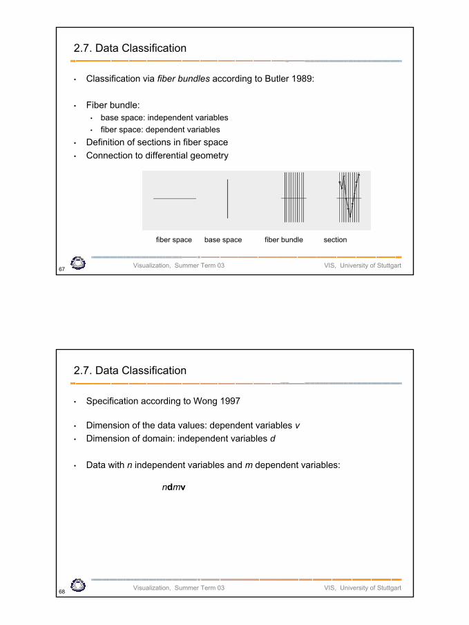
2.7. Data Classification
• Classification via fiber bundles according to Butler 1989:
• Fiber bundle:• base space: independent variables• fiber space: dependent variables
• Definition of sections in fiber space• Connection to differential geometry
fiber space base space fiber bundle section
Visualization, Summer Term 03 VIS, University of Stuttgart68
2.7. Data Classification
• Specification according to Wong 1997
• Dimension of the data values: dependent variables v• Dimension of domain: independent variables d
• Data with n independent variables and m dependent variables:
ndmv
Visualization, Summer Term 2002 20.05.2003
35
Visualization, Summer Term 03 VIS, University of Stuttgart69
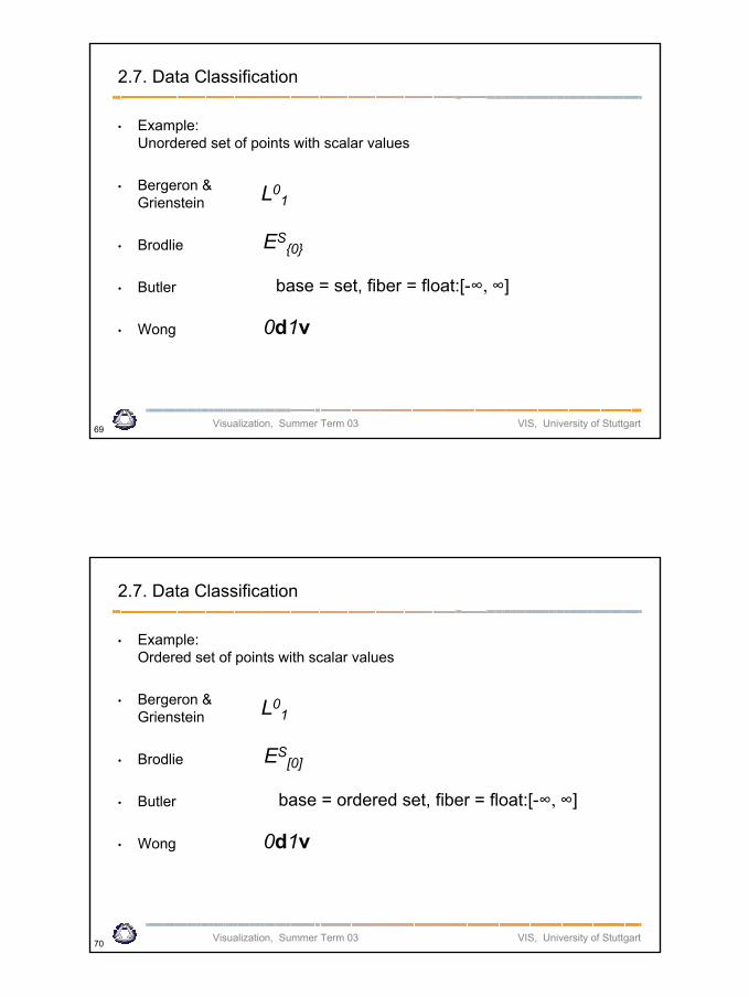
2.7. Data Classification
• Example:Unordered set of points with scalar values
• Bergeron &Grienstein
• Brodlie
• Butler
• Wong
L01
ES{0}
base = set, fiber = float:[-∞, ∞]
0d1v
Visualization, Summer Term 03 VIS, University of Stuttgart70
2.7. Data Classification
• Example:Ordered set of points with scalar values
• Bergeron &Grienstein
• Brodlie
• Butler
• Wong
L01
ES[0]
base = ordered set, fiber = float:[-∞, ∞]
0d1v
Visualization, Summer Term 2002 20.05.2003
36
Visualization, Summer Term 03 VIS, University of Stuttgart71
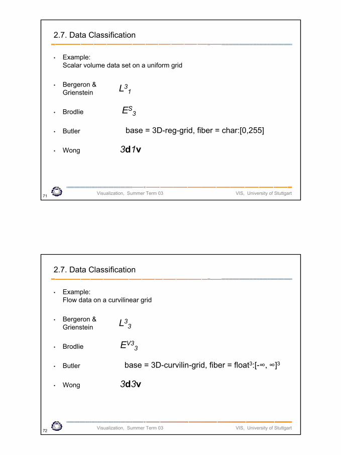
2.7. Data Classification
• Example:Scalar volume data set on a uniform grid
• Bergeron &Grienstein
• Brodlie
• Butler
• Wong
L31
ES3
base = 3D-reg-grid, fiber = char:[0,255]
3d1v
Visualization, Summer Term 03 VIS, University of Stuttgart72
2.7. Data Classification
• Example:Flow data on a curvilinear grid
• Bergeron &Grienstein
• Brodlie
• Butler
• Wong
L33
EV33
base = 3D-curvilin-grid, fiber = float3:[-∞, ∞]3
3d3v
Visualization, Summer Term 2002 20.05.2003
37
Visualization, Summer Term 03 VIS, University of Stuttgart73
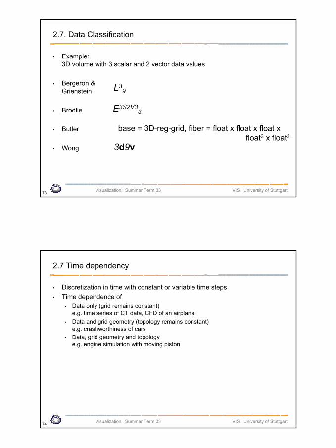
2.7. Data Classification
• Example:3D volume with 3 scalar and 2 vector data values
• Bergeron &Grienstein
• Brodlie
• Butler
• Wong
L39
E3S2V33
base = 3D-reg-grid, fiber = float x float x float x float3 x float3
3d9v
Visualization, Summer Term 03 VIS, University of Stuttgart74
2.7 Time dependency
• Discretization in time with constant or variable time steps• Time dependence of
• Data only (grid remains constant)e.g. time series of CT data, CFD of an airplane
• Data and grid geometry (topology remains constant)e.g. crashworthiness of cars
• Data, grid geometry and topologye.g. engine simulation with moving piston
Visualization, Summer Term 2002 20.05.2003
38
Visualization, Summer Term 03 VIS, University of Stuttgart75
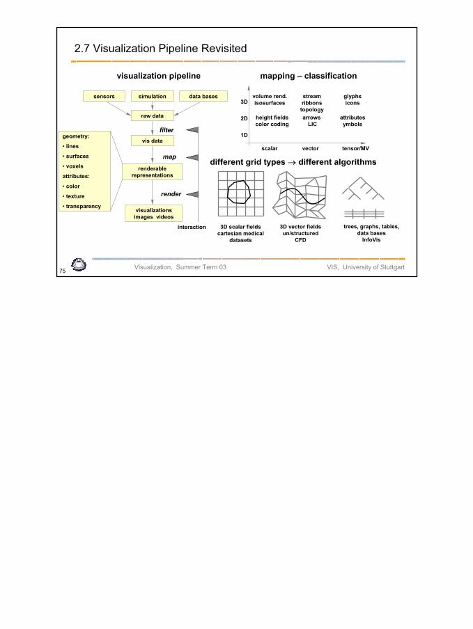
2.7 Visualization Pipeline Revisited
sensors data basessimulation
raw data
vis data
renderablerepresentations
visualizationsimages videos
geometry:
• lines
• surfaces
• voxels
attributes:
• color
• texture
• transparency
filter
render
map
interaction
visualization pipeline mapping – classification
1D
3D
2D
scalar vector tensor/MV
volume rend. isosurfaces
height fields color coding
stream ribbons
topologyarrows
LICattributesymbols
glyphs icons
different grid types → different algorithms
3D scalar fieldscartesian medical
datasets
3D vector fields un/structured
CFD
trees, graphs, tables, data bases
InfoVis