18-759: wireless networks cellular versus wifi overview the
TRANSCRIPT
Page 1
Peter A. Steenkiste, CMU 1
18-759: Wireless NetworksLecture 16: Cellular
Peter SteenkisteDepartments of Computer Science andElectrical and Computer Engineering
Spring Semester 2016http://www.cs.cmu.edu/~prs/wirelessS16/
Peter A. Steenkiste, CMU 2
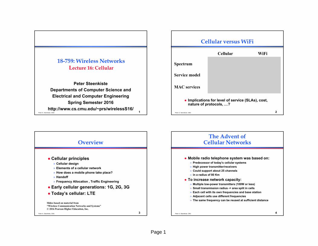
Cellular versus WiFi
Implications for level of service (SLAs), cost, nature of protocols, …?
Spectrum
Service model
MAC services
Cellular
Licensed
Provisioned“for pay”
Fixed bandwidthSLAs
WiFi
Unlicensed
Unprovisioned“free” – no SLA
Best effortno SLAs
Peter A. Steenkiste, CMU 3
Overview
Cellular principles» Cellular design» Elements of a cellular network» How does a mobile phone take place?» Handoff» Frequency Allocation , Traffic Engineering
Early cellular generations: 1G, 2G, 3G Today’s cellular: LTE
Slides based on material from “Wireless Communication Networks and Systems”© 2016 Pearson Higher Education, Inc.
Peter A. Steenkiste, CMU 4
The Advent of Cellular Networks
Mobile radio telephone system was based on:» Predecessor of today’s cellular systems» High power transmitter/receivers» Could support about 25 channels » in a radius of 80 Km
To increase network capacity:» Multiple low-power transmitters (100W or less)» Small transmission radius -> area split in cells» Each cell with its own frequencies and base station» Adjacent cells use different frequencies» The same frequency can be reused at sufficient distance
Page 2
Peter A. Steenkiste, CMU 5
Cellular Network Design Options
Simplest layout» Adjacent antennas not
equidistant – how do you handle users at the edge of the cell?
Ideal layout» But we know signals
travel whatever way they feel like
» Does not cover entire area
dd √2d
d
d
Peter A. Steenkiste, CMU 6
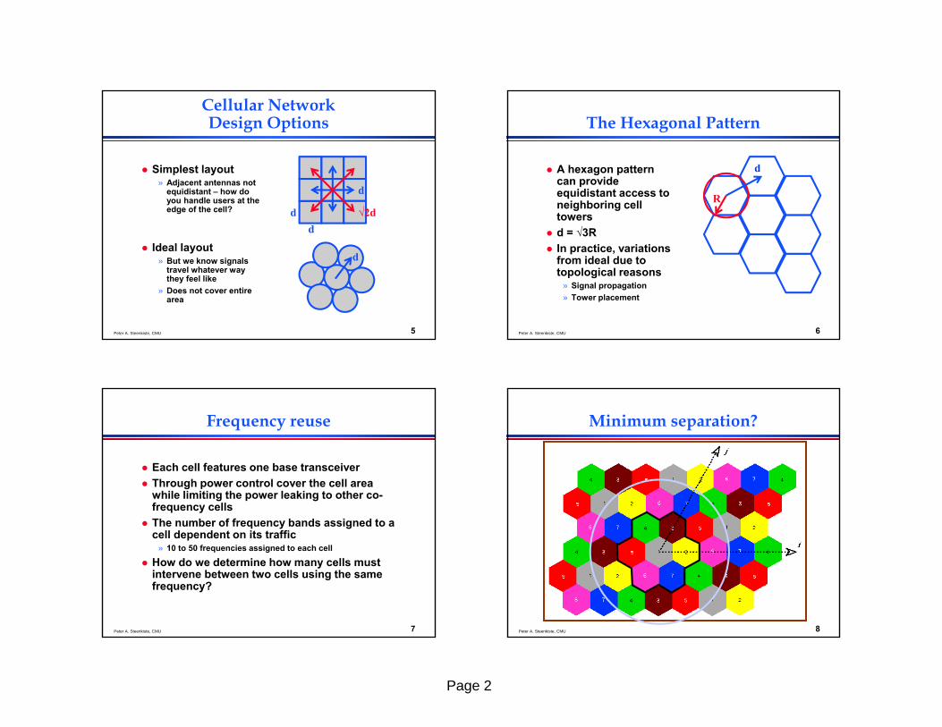
The Hexagonal Pattern
A hexagon pattern can provide equidistant access to neighboring cell towers
d = √3R In practice, variations
from ideal due to topological reasons
» Signal propagation» Tower placement
d
R
Peter A. Steenkiste, CMU 7
Frequency reuse
Each cell features one base transceiver Through power control cover the cell area
while limiting the power leaking to other co-frequency cells
The number of frequency bands assigned to a cell dependent on its traffic
» 10 to 50 frequencies assigned to each cell
How do we determine how many cells must intervene between two cells using the same frequency?
Peter A. Steenkiste, CMU 8
Minimum separation?
Page 3
Peter A. Steenkiste, CMU 9
Frequency reuse characterization
D = minimum distance between centers of co-channel cells
R = radius of cell d = distance between centers of adjacent cells N = number of cells in a repetitious pattern, i.e.
reuse factor Hexagonal pattern only possible for certain N:
The following relationship holdN I2J2(IJ), I,J0,1,2,3,...
DR 3N or D
d N
Peter A. Steenkiste, CMU 10
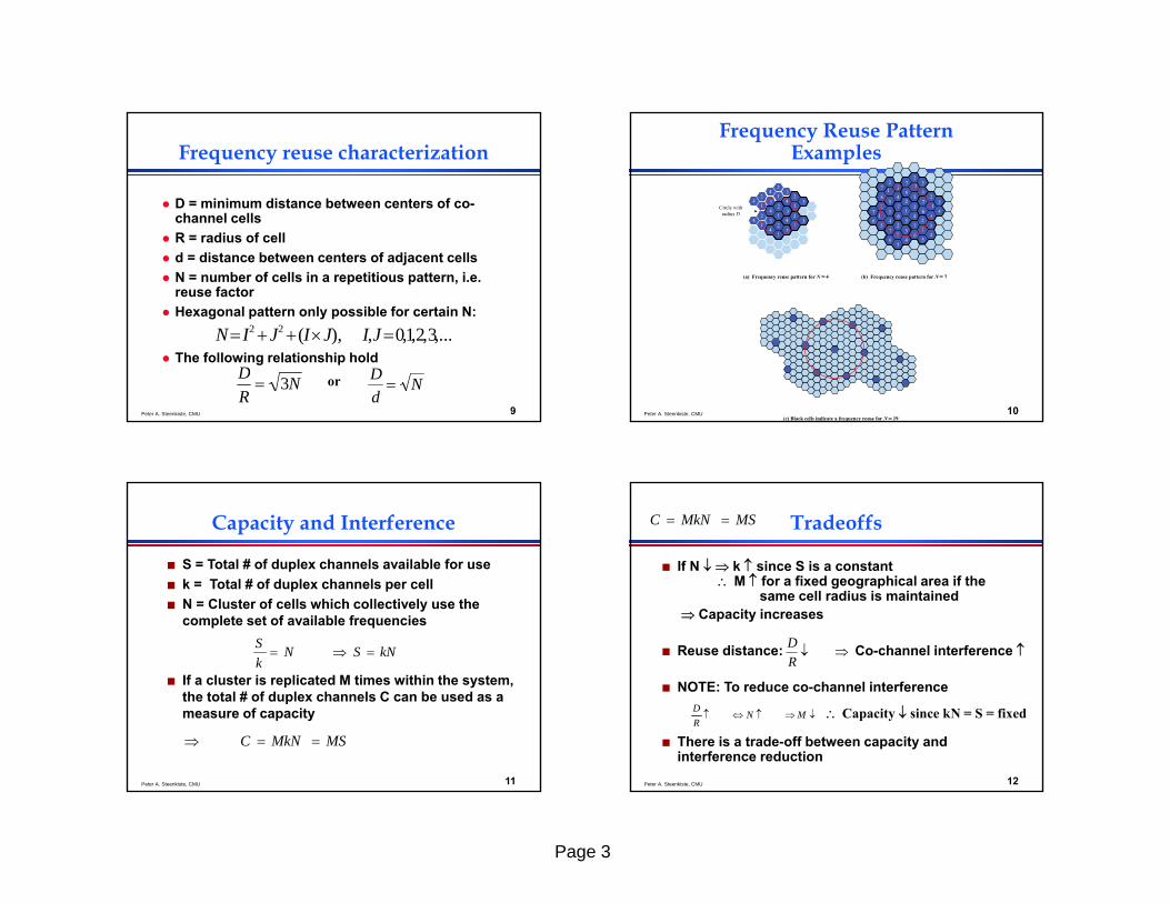
Frequency Reuse Pattern Examples
Peter A. Steenkiste, CMU 11
Capacity and Interference
S = Total # of duplex channels available for use k = Total # of duplex channels per cell N = Cluster of cells which collectively use the
complete set of available frequencies
If a cluster is replicated M times within the system, the total # of duplex channels C can be used as a measure of capacity
kNSNkS
MSMkNC
Peter A. Steenkiste, CMU 12
Tradeoffs
If N k since S is a constant M for a fixed geographical area if the
same cell radius is maintained Capacity increases
Reuse distance: Co-channel interference
NOTE: To reduce co-channel interference
There is a trade-off between capacity and interference reduction
RD
MNRD Capacity since kN = S = fixed
MSMkNC
Page 4
Peter A. Steenkiste, CMU 13
Approaches to Cope with Increasing Capacity
Adding new channels Frequency borrowing – frequencies are taken from
adjacent cells by congested cells Cell splitting – cells in areas of high usage can be
split into smaller cells Cell sectoring – cells are divided into wedge-shaped
sectors, each with their own set of channels Network densification – more cells and frequency
reuse» Microcells – antennas move to buildings, hills, and lamp posts» Femtocells – antennas to create small cells in buildings
Peter A. Steenkiste, CMU 14
More Advanced Techniques
Interference coordination – tighter control of interference so frequencies can be reused closer to other base stations
» Inter-cell interference coordination (ICIC)» Coordinated multipoint transmission (CoMP)
Peter A. Steenkiste, CMU 15
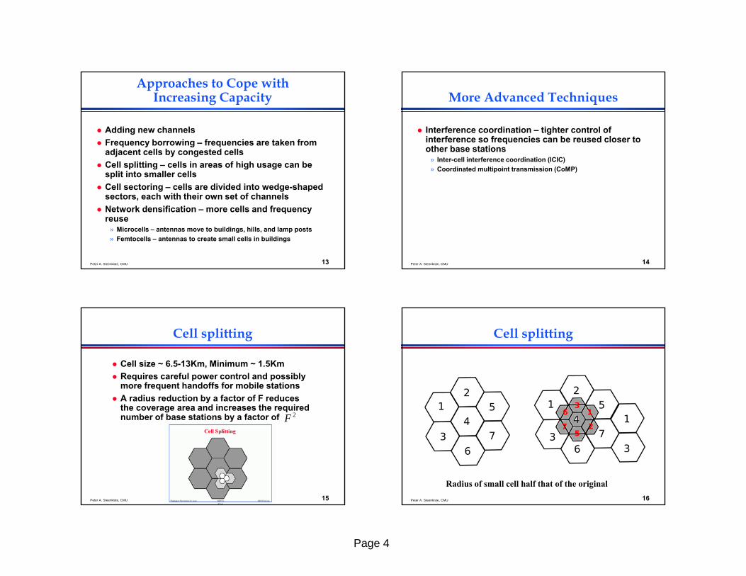
Cell splitting
Cell size ~ 6.5-13Km, Minimum ~ 1.5Km Requires careful power control and possibly
more frequent handoffs for mobile stations A radius reduction by a factor of F reduces
the coverage area and increases the required number of base stations by a factor of F 2
Peter A. Steenkiste, CMU 16
Cell splitting
Radius of small cell half that of the original
Page 5
Peter A. Steenkiste, CMU 17
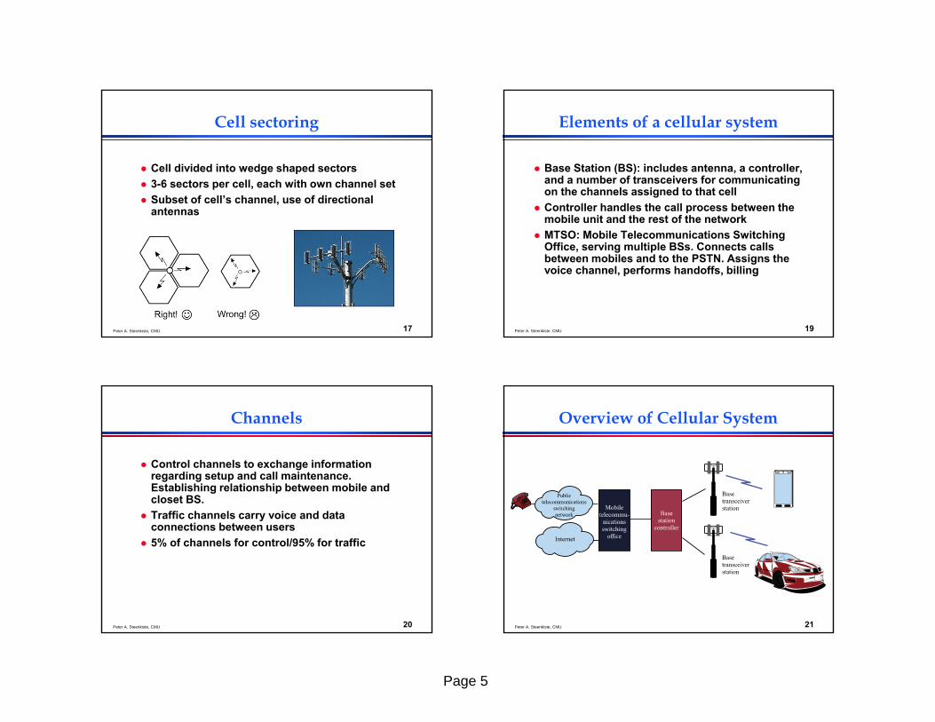
Cell sectoring
Cell divided into wedge shaped sectors 3-6 sectors per cell, each with own channel set Subset of cell’s channel, use of directional
antennas
Peter A. Steenkiste, CMU 19
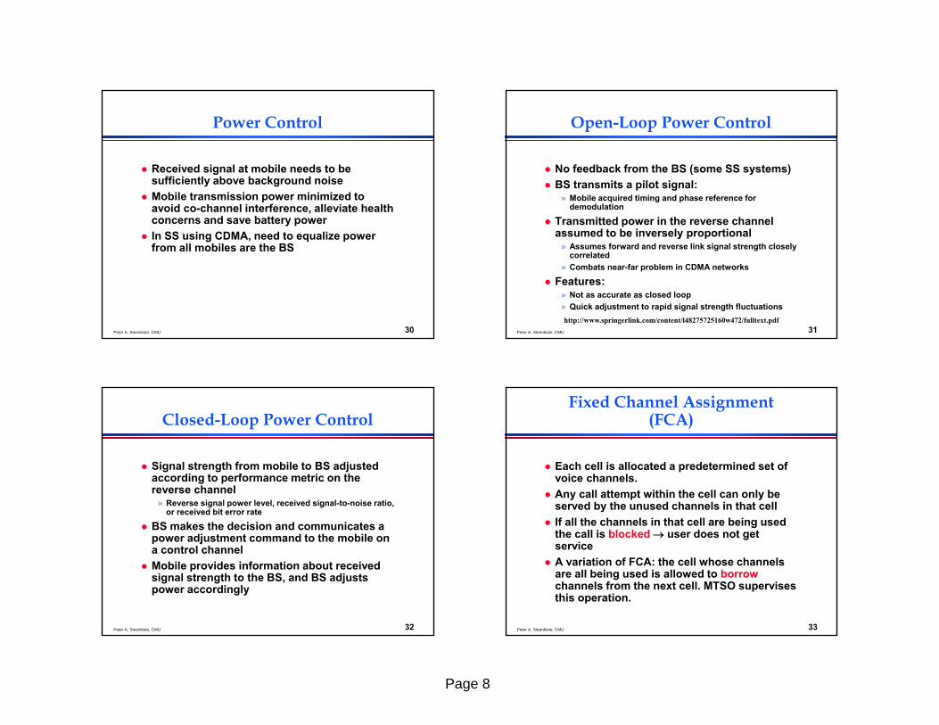
Elements of a cellular system
Base Station (BS): includes antenna, a controller, and a number of transceivers for communicating on the channels assigned to that cell
Controller handles the call process between the mobile unit and the rest of the network
MTSO: Mobile Telecommunications Switching Office, serving multiple BSs. Connects calls between mobiles and to the PSTN. Assigns the voice channel, performs handoffs, billing
Peter A. Steenkiste, CMU 20
Channels
Control channels to exchange information regarding setup and call maintenance. Establishing relationship between mobile and closet BS.
Traffic channels carry voice and data connections between users
5% of channels for control/95% for traffic
Peter A. Steenkiste, CMU 21
Overview of Cellular System
Page 6
Peter A. Steenkiste, CMU 22
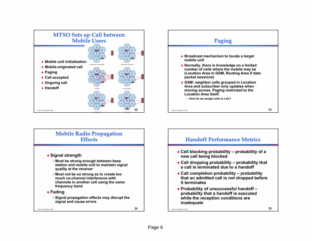
MTSO Sets up Call between Mobile Users
Mobile unit initialization Mobile-originated call Paging Call accepted Ongoing call Handoff
Peter A. Steenkiste, CMU 23
Paging
Broadcast mechanism to locate a target mobile unit
Normally, there is knowledge on a limited number of cells where the mobile may be (Location Area in GSM, Routing Area if data packet sessions)
GSM: neighbor cells grouped in Location Area and subscriber only updates when moving across. Paging restricted to the Location Area itself.
» How do we assign cells to LAs?
Peter A. Steenkiste, CMU 24
Mobile Radio Propagation Effects
Signal strength» Must be strong enough between base
station and mobile unit to maintain signal quality at the receiver
» Must not be so strong as to create too much co-channel interference with channels in another cell using the same frequency band
Fading» Signal propagation effects may disrupt the
signal and cause errors
Peter A. Steenkiste, CMU 25
Handoff Performance Metrics
Cell blocking probability – probability of a new call being blocked
Call dropping probability – probability that a call is terminated due to a handoff
Call completion probability – probability that an admitted call is not dropped before it terminates
Probability of unsuccessful handoff –probability that a handoff is executed while the reception conditions are inadequate
Page 7
Peter A. Steenkiste, CMU 26
Handoff Performance Metrics
Handoff blocking probability – probability that a handoff cannot be successfully completed
Handoff probability – probability that a handoff occurs before call termination
Rate of handoff – number of handoffs per unit time
Interruption duration – duration of time during a handoff in which a mobile is not connected to either base station
Handoff delay – distance the mobile moves from the point at which the handoff should occur to the point at which it does occur
Peter A. Steenkiste, CMU 27
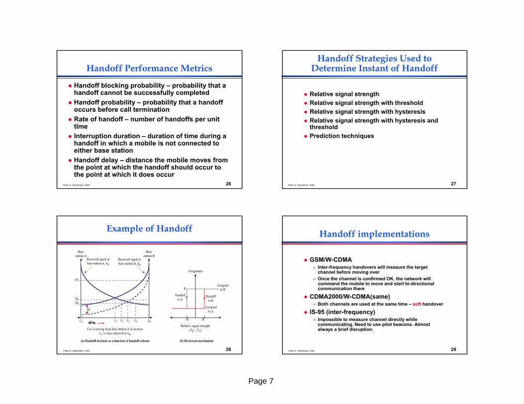
Handoff Strategies Used to Determine Instant of Handoff
Relative signal strength Relative signal strength with threshold Relative signal strength with hysteresis Relative signal strength with hysteresis and
threshold Prediction techniques
Peter A. Steenkiste, CMU 28
Example of Handoff
Peter A. Steenkiste, CMU 29
Handoff implementations
GSM/W-CDMA» Inter-frequency handovers will measure the target
channel before moving over» Once the channel is confirmed OK, the network will
command the mobile to move and start bi-directional communication there
CDMA2000/W-CDMA(same)» Both channels are used at the same time – soft handover
IS-95 (inter-frequency)» Impossible to measure channel directly while
communicating. Need to use pilot beacons. Almost always a brief disruption.
Page 8
Peter A. Steenkiste, CMU 30
Power Control
Received signal at mobile needs to be sufficiently above background noise
Mobile transmission power minimized to avoid co-channel interference, alleviate health concerns and save battery power
In SS using CDMA, need to equalize power from all mobiles are the BS
Peter A. Steenkiste, CMU 31
Open-Loop Power Control
No feedback from the BS (some SS systems) BS transmits a pilot signal:
» Mobile acquired timing and phase reference for demodulation
Transmitted power in the reverse channel assumed to be inversely proportional
» Assumes forward and reverse link signal strength closely correlated
» Combats near-far problem in CDMA networks
Features:» Not as accurate as closed loop» Quick adjustment to rapid signal strength fluctuationshttp://www.springerlink.com/content/l48275725160w472/fulltext.pdf
Peter A. Steenkiste, CMU 32
Closed-Loop Power Control
Signal strength from mobile to BS adjusted according to performance metric on the reverse channel
» Reverse signal power level, received signal-to-noise ratio, or received bit error rate
BS makes the decision and communicates a power adjustment command to the mobile on a control channel
Mobile provides information about received signal strength to the BS, and BS adjusts power accordingly
Peter A. Steenkiste, CMU 33
Fixed Channel Assignment (FCA)
Each cell is allocated a predetermined set of voice channels.
Any call attempt within the cell can only be served by the unused channels in that cell
If all the channels in that cell are being used the call is blocked user does not get service
A variation of FCA: the cell whose channels are all being used is allowed to borrow channels from the next cell. MTSO supervises this operation.
Page 9
Peter A. Steenkiste, CMU 34
Dynamic Channel Assignment (DCA)
Voice channels are not assigned or allocated to different cells permanently. Instead each time a request is made, the serving BS requests a channel from the MTSO.
MTSO allocates a channel to the requested cell following an algorithm that takes into account the likelihood of future blocking within the cell, the freq. of use of the candidate channel, the reuse distance of the channel, and other cost functions.
MTSO only allocates a channel if it is available and not being used in the restricted distance for co-channel interference
Peter A. Steenkiste, CMU 35
FCA/DCA comparison
Advantage of DCA: Likelihood of blocking decreases and trunking efficiency increases
Disadvantage of DCA: MTSO should collect real-time data on channel occupancy, traffic distribution and RSSI of all channels on a continuous basis.
Overhead in terms of storage and computational load on the system.
Peter A. Steenkiste, CMU 36
Traffic Engineering
If the cell has L subscribers.. … and can support N simultaneous users. If L<=N, nonblocking system If L>N, blocking system Questions operator cares about:
» What is the probability of a call being blocked?» What N do I need to upper bound this probability?» If blocked calls are queued, what is the average delay?» What capacity is needed to achieve a certain average
delay?
Peter A. Steenkiste, CMU 37
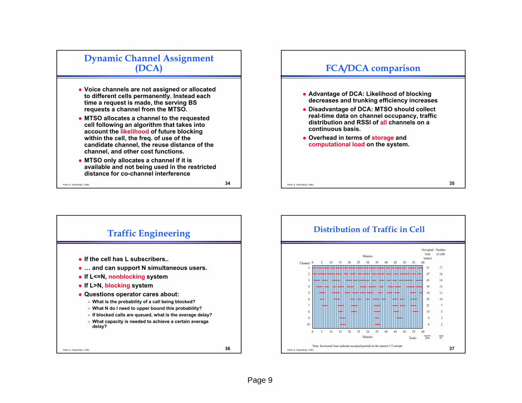
Distribution of Traffic in Cell
Page 10
Peter A. Steenkiste, CMU 38
Blocking System Performance Questions
Probability that call request is blocked? What capacity is needed to achieve a certain
upper bound on probability of blocking? What is the average delay? What capacity is needed to achieve a certain
average delay?
Peter A. Steenkiste, CMU 39
Trunking Theory Terminology
Set-up Time: The time required to allocated a trunked radio channel to a requesting user.
Blocked Call (Lost Call): Call that cannot be completed at time of request, due to congestion.
Holding Time: Average duration of a typical call. Denoted by h (in seconds).
Traffic Intensity: Measure of channel time utilization, which is the average channel occupancy measured in Erlangs.
Peter A. Steenkiste, CMU 40
Trunking Theory Terminology
Load: Traffic intensity across the entire trunked radio system, measured in Erlangs.
Grade of Service (GOS): A measure of congestion specified as the probability of a call being blocked (for Erlang B), or the probability of a call being delayed beyond a certain amount of time (for Erlang C).
Request Rate: The average number of call requests per unit time. Denoted by λ calls per second.
Peter A. Steenkiste, CMU 41
Trunking Theory
Traffic intensity: A = λh » λ is the mean rate of calls attempted per time unit» h is the mean holding time per successful call
If channel capacity is N – system can be seen as a multiserver queuing system
λh = ρNρ is server utilization, fraction of time server is busy
A also average number of channels required
Page 11
Peter A. Steenkiste, CMU 42
Simple Example
A cell has a capacity of 10 channels In 1 hour it received 97 calls lasting 294
minutes in total The rate of calls per min = 97/60 The average holding time = 294/97 A = (97/60) x (294/97) = 4.9 Erlangs
Mean number of calls in progress is 4.9 Mean number of channels engaged is 4.9
Peter A. Steenkiste, CMU 43
Cellular Network Design
Sized to sustain the average demand in the busy hour (not peak demand!)
Based on carried traffic and not offered! Model depends on:
» How are blocked calls handled?– Could be put in a queue (lost calls delayed)– Rejected or dropped 1. user may hang up and try again after some random
time interval – lost calls cleared (LCC)2. User repeatedly attempts – lost calls held (LCH)
» Number of traffic sources– Finite or infinite?– Infinite source assumption reasonable when sources
at least 5 to 10 times the capacity of the system
Peter A. Steenkiste, CMU 44
Infinite Source LLC –Grade of Service
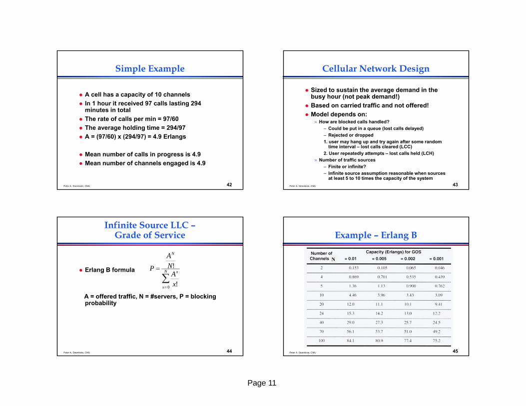
Erlang B formula
A = offered traffic, N = #servers, P = blocking probability
P
AN
N!Ax
x!x 0
N
Peter A. Steenkiste, CMU 45
Example – Erlang B
N
Page 12
Peter A. Steenkiste, CMU 46
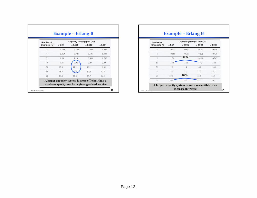
Example – Erlang B
N
A larger capacity system is more efficient than a smaller-capacity one for a given grade of service
Peter A. Steenkiste, CMU 47
Example – Erlang B
N
A larger capacity system is more susceptible to an increase in traffic
30%
10%