16. A Logistic Regression Illustration

36-402, Advanced Data Analysis

22 March 2011

The first part of lecture today was review and reinforcement of the gen-eral ideas about logistic regression and other GLMs from the previous lectures.These notes elaborate on the example I did in class, of building and testing aGLM (specifically, a logistic regression model) for a particular data set.

Specifically, we are going to build a simple weather forecaster. Our dataconsist of daily records, from the beginning of 1948 to the end of 1983, of pre-cipitation at Snoqualmie Falls, Washington1. Each row of the data file is adifferent year; each column records, for that day of the year, the day’s precipi-tation (rain or snow), in units of 1

100 inch. Because of leap-days, there are 366columns, with the last column having an NA value for three out of four years.

snoqualmie <- read.csv("snoqualmie.csv",header=FALSE)snoqualmie <- unlist(snoqualmie) # Turn into one big vector without year breakssnoqualmie <- na.omit(snoqualmie) # Remove NAs from non-leap-years

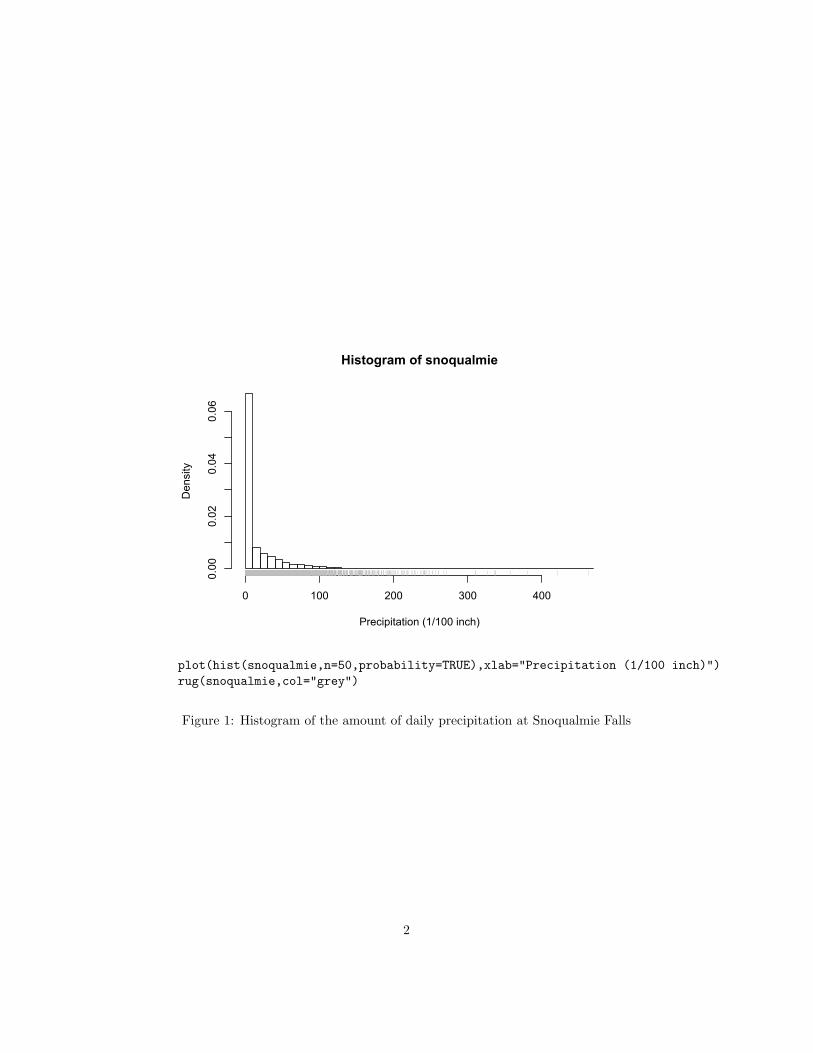
What we want to do is predict tomorrow’s weather from today’s. Thiswould be of interest if we lived in Snoqualmie Falls, or if we operated eitherone of the local hydroelectric power plants, or the tourist attraction of the Fallsthemselves. Examining the distribution of the data (Figures 1 and 2) showsthat there is a big spike in the distribution at zero precipitation, and that daysof no precipitation can follow days of any amount of precipitation but seem tobe less common after heavy precipitation.

These facts suggest that “no precipitation” is a special sort of event whichwould be worth predicting in its own right (as opposed to just being whenthe precipitation happens to be zero), so we will attempt to do so with logisticregression. Specifically, the input variable Xi will be the amount of precipitationon the ith day, and the response Yi will be the indicator variable for whetherthere was any precipitation on day i+1 — that is, Yi = 1 if Xi+1 > 0, an Yi = 0if Xi+1 = 0. We expect from Figure 2, as well as common experience, that thecoefficient on X should be positive.2

Before fitting the logistic regression, it’s convenient to re-shape the data:1I learned of this data set from Peter Guttorp’s Stochastic Modeling of Scientific Data; the

data file is available from http://www.stat.washington.edu/peter/stoch.mod.data.html.2This does not attempt to model how much precipitation there will be tomorrow, if there

is any. We could make that a separate model, if we can get this part right.

1

Histogram of snoqualmie

Precipitation (1/100 inch)

Density

0 100 200 300 400

0.00

0.02

0.04

0.06

plot(hist(snoqualmie,n=50,probability=TRUE),xlab="Precipitation (1/100 inch)")rug(snoqualmie,col="grey")

Figure 1: Histogram of the amount of daily precipitation at Snoqualmie Falls

2

0 100 200 300 400

0100

200

300

400

Precipitation today (1/100 inch)

Pre

cipi

tatio

n to

mor

row

(1/1

00 in

ch)

plot(snoqualmie[-length(snoqualmie)],snoqualmie[-1],xlab="Precipitation today (1/100 inch)",ylab="Precipitation tomorrow (1/100 inch)",cex=0.1)

rug(snoqualmie[-length(snoqualmie)],side=1,col="grey")rug(snoqualmie[-1],side=2,col="grey")

Figure 2: Scatterplot showing relationship between amount of precipitation onsuccessive days. Notice that days of no precipitation can follow days of anyamount of precipitation, but seem to be more common when there is little orno precipitation to start with.

3

vector.to.pairs <- function(v) {v <- as.numeric(v)n <- length(v)return(cbind(v[-1],v[-n]))

}snoq.pairs <- vector.to.pairs(snoqualmie)colnames(snoq.pairs) <- c("tomorrow","today")snoq <- as.data.frame(snoq.pairs)

This creates a two-column array, where the first column is the precipitation onday i+1, and the second column is the precipitation on day i (hence the columnnames). Finally, I turn the whole thing into a data frame.

Now fitting is straightforward:

snoq.logistic <- glm((tomorrow > 0) ~ today, data=snoq, family=binomial)

To see what came from the fitting, run summary:

> summary(snoq.logistic)

Call:glm(formula = (tomorrow > 0) ~ today, family = binomial, data = snoq)

Deviance Residuals:Min 1Q Median 3Q Max

-2.3713 -1.1805 0.9536 1.1693 1.1744

Coefficients:Estimate Std. Error z value Pr(>|z|)

(Intercept) 0.0071899 0.0198430 0.362 0.717today 0.0059232 0.0005858 10.111 <2e-16 ***---

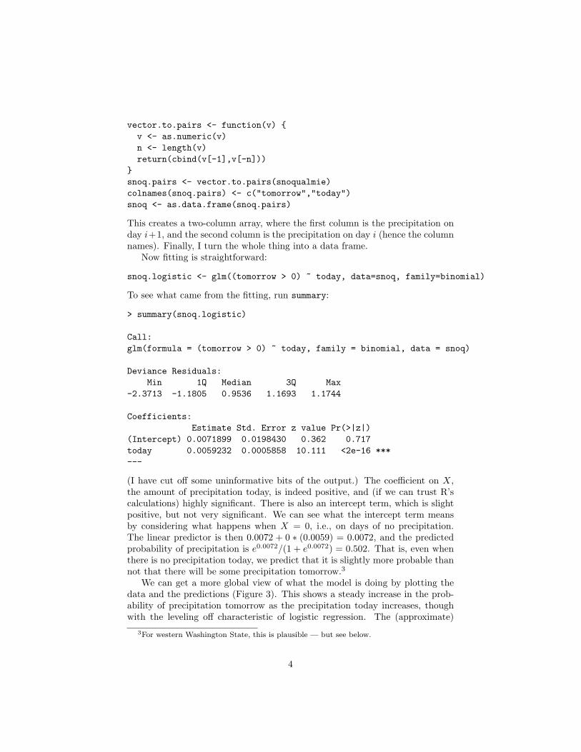
(I have cut off some uninformative bits of the output.) The coefficient on X,the amount of precipitation today, is indeed positive, and (if we can trust R’scalculations) highly significant. There is also an intercept term, which is slightpositive, but not very significant. We can see what the intercept term meansby considering what happens when X = 0, i.e., on days of no precipitation.The linear predictor is then 0.0072 + 0 ∗ (0.0059) = 0.0072, and the predictedprobability of precipitation is e0.0072/(1 + e0.0072) = 0.502. That is, even whenthere is no precipitation today, we predict that it is slightly more probable thannot that there will be some precipitation tomorrow.3

We can get a more global view of what the model is doing by plotting thedata and the predictions (Figure 3). This shows a steady increase in the prob-ability of precipitation tomorrow as the precipitation today increases, thoughwith the leveling off characteristic of logistic regression. The (approximate)

3For western Washington State, this is plausible — but see below.

4

95% confidence limits for the predicted probability are (on close inspection)asymmetric, and actually slightly narrower at the far right than at intermediatevalues of X (Figure ).

How well does this work? We can get a first sense of this by comparingit to a simple nonparametric smoothing of the data. Remembering that whenY is binary, Pr Y = 1|X = x = E [Y |X = x], we can use a smoothing spline toestimate E [Y |X = x] (Figure 5). This would not be so great as a model — itignores the fact that the response is a binary event and we’re trying to estimatea probability, the fact that the variance of Y therefore depends on its mean, etc.— but it’s at least indicative.

The result is in not-terribly-bad agreement with the logistic regression up toabout 1.2 or 1.3 inches of precipitation, after which it runs significantly belowthe logistic regression, rejoins it around 3.5 inches of precipitation, and then (asit were) falls off a cliff.

We can do better by fitting a generalized additive model. In this case,with only one predictor variable, this means using non-parametric smoothing toestimate the log odds — we’re still using the logistic transformation, but onlyrequiring that the log odds change smoothly with X, not that they be linear inX. The result (Figure 6) is actually quite similar to the spline, but a bit betterbehaved, and has confidence intervals. At the largest values of X, the latterspan nearly the whole range from 0 to 1, which is not unreasonable consideringthe sheer lack of data there.

Visually, the logistic regression curve is usually but not always within theconfidence limits of the non-parametric predictor. What can we say about thedifference between the two models more quantiatively?

Numerically, the deviance is 18079.69 for the logistic regression, and 18036.77for the GAM. We can go through the testing procedure outlined in the notesfor lecture 14. We need a simulator (which presumes that the logistic regressionmodel is true), and we need to calculate the difference in deviance on simulateddata many times.

# Simulate from the fitted logistic regression model for Snoqualmie# Presumes: fitted values of the model are probabilities.snoq.sim <- function(model=snoq.logistic) {fitted.probs <- fitted(model)n <- length(fitted.probs)new.binary <- rbinom(n,size=1,prob=fitted.probs)return(new.binary)

}

A quick check of the simulator against the observed values:

> summary(ifelse(snoq[,1]>0,1,0))Min. 1st Qu. Median Mean 3rd Qu. Max.

0.0000 0.0000 1.0000 0.5262 1.0000 1.0000> summary(snoq.sim())

Min. 1st Qu. Median Mean 3rd Qu. Max.

5

0 100 200 300 400

0.0

0.2

0.4

0.6

0.8

1.0

Precipitation today (1/100 inch)

Pos

itive

pre

cipi

tatio

n to

mor

row

?

plot((tomorrow>0)~today,data=snoq,xlab="Precipitation today (1/100 inch)",ylab="Positive precipitation tomorrow?")

rug(snoq$today,side=1,col="grey")

data.plot <- data.frame(today=(0:500))logistic.predictions <- predict(snoq.logistic,newdata=data.plot,se.fit=TRUE)lines(0:500,ilogit(logistic.predictions$fit))lines(0:500,ilogit(logistic.predictions$fit+1.96*logistic.predictions$se.fit),

lty=2)lines(0:500,ilogit(logistic.predictions$fit-1.96*logistic.predictions$se.fit),

lty=2)

Figure 3: Data (dots), plus predicted probabilities (solid line) and approximate95% confidence intervals from the logistic regression model (dashed lines). Notethat calculating standard errors for predictions on the logit scale, and thentransforming, is better practice than getting standard errors directly on theprobability scale.

6

0 100 200 300 400 500

0.01

0.02

0.03

0.04

Difference in probability between prediction and confidence limit for prediction

Precipitation today (1/100 inch)

Δprobability

plot(0:500,ilogit(logistic.predictions$fit)-ilogit(logistic.predictions$fit-1.96*logistic.predictions$se.fit),

type="l",col="blue",xlab="Precipitation today (1/100 inch)",main="Difference in probability between prediction\n

and confidence limit for prediction",ylab = expression(paste(Delta,"probability")))

lines(0:500,ilogit(logistic.predictions$fit+1.96*logistic.predictions$se.fit)-ilogit(logistic.predictions$fit))

Figure 4: Distance from the fitted probability to the upper (black) and lower(blue) confidence limits. Notice that the two are not equal, and somewhatsmaller at very large values of X than at intermediate ones. (Why?)

7

0 100 200 300 400

0.0

0.2

0.4

0.6

0.8

1.0

Precipitation today (1/100 inch)

Pos

itive

pre

cipi

tatio

n to

mor

row

?

snoq.spline <- smooth.spline(x=snoq$today,y=(snoq$tomorrow>0))lines(snoq.spline,col="red")

Figure 5: As Figure 3, plus a smoothing spline (red).

8

0 100 200 300 400

0.0

0.2

0.4

0.6

0.8

1.0

Precipitation today (1/100 inch)

Pos

itive

pre

cipi

tatio

n to

mor

row

?

library(mgcv)snoq.gam <- gam((tomorrow>0)~s(today),data=snoq,family=binomial)gam.predictions <- predict.gam(snoq.gam,newdata=data.plot,se.fit=TRUE)lines(0:500,ilogit(gam.predictions$fit),col="blue")lines(0:500,ilogit(gam.predictions$fit+1.96*gam.predictions$se.fit),

col="blue",lty=2)lines(0:500,ilogit(gam.predictions$fit-1.96*gam.predictions$se.fit),

col="blue",lty=2)

Figure 6: As Figure 5, but with the addition of a generalized additive model(blue line) and its confidence limits (dashed blue lines). Note: the predictfunction in the gam package does not allow one to calculate standard er-rors for new data. You may need to un-load the gam library first, withdetach(package:gam).

9

0.0000 0.0000 1.0000 0.5264 1.0000 1.0000

This suggests that the simulator is not acting crazily.Now for the difference in deviances:

# Simulate from fitted logistic regression, re-fit logistic regression and# GAM, calculate difference in deviancesdiff.dev <- function(model=snoq.logistic,x=snoq[,2]) {y.new <- snoq.sim(model)GLM.dev <- glm(y.new ~ x,family=binomial)$devianceGAM.dev <- gam(y.new ~ s(x),family=binomial)$deviancereturn(GLM.dev-GAM.dev)

}

A single run of this takes about 1.5 seconds on my computer.Finally, we calculate the distribution of difference in deviances under the

null (that the logistic regression is properly specified), and the correspondingp-value:

diff.dev.obs <- snoq.logistic$deviance - snoq.gam$deviancenull.dist.of.diff.dev <- replicate(1000,diff.dev())p.value <- (1+sum(null.dist.of.diff.dev > diff.dev.obs))/(1+length(null.dist.of.diff.dev))

Using a thousand replicates takes about 1500 seconds, or roughly 25 minutes,which is substantial, but not impossible; it gave a p-value of < 10−3, and thefollowing sampling distribution:

> summary(null.dist.of.diff.dev)Min. 1st Qu. Median Mean 3rd Qu. Max.

0.000097 0.002890 0.016770 2.267000 2.897000 29.750000

(A preliminary trial run of only 100 replicates, taking a few minutes, gave

> summary(null.dist.of.diff.dev)Min. 1st Qu. Median Mean 3rd Qu. Max.

0.000291 0.002681 0.013700 2.008000 2.121000 27.820000

which implies a p-value of < 0.01. This would be good enough for many practicalpurposes.)

Having detected that there is a problem with the GLM, we can ask whereit lies. We could just use the GAM, but it’s more interesting to try to diagnosewhat’s going on.

In this respect Figure 6 is actually a little misleading, because it leads the eyeto emphasize the disagreement between the models at large X, when actuallythere are very few data points there, and so even large differences in predictedprobabilities there contribute little to the over-all likelihood difference. Whatis actually more important is what happens at X = 0, which contains a verylarge number of observations (about 47% of all observations), and which wehave reason to think is a special value anyway.

10

Let’s try introducing a dummy variable for X = 0 into the logistic regression,and see what happens. It will be convenient to augment the data frame withan extra column, recording 1 whenever X = 0 and 0 otherwise.

snoq2 <- data.frame(snoq,dry=ifelse(snoq$today==0,1,0))snoq2.logistic <- glm((tomorrow > 0) ~ today + dry,data=snoq2,family=binomial)snoq2.gam <- gam((tomorrow > 0) ~ s(today) + dry,data=snoq2,family=binomial)

Notice that I allow the GAM to treat zero as a special value as well, by givingit access to that dummy variable. In principle, with enough data it can decidewhether or not that is useful on its own, but since we have guessed that it is, wemight as well include it. Figure 7 shows the data and the two new models. Theseare extremely close to each other. The new GLM has a deviance of 18015.65,lower than even the GAM before, and the new GAM has a deviance of 18015.21.The p-value is essentially 1 — and yet we know that the test, with this test,does have power to detect departures from the parametric model. This is verypromising.

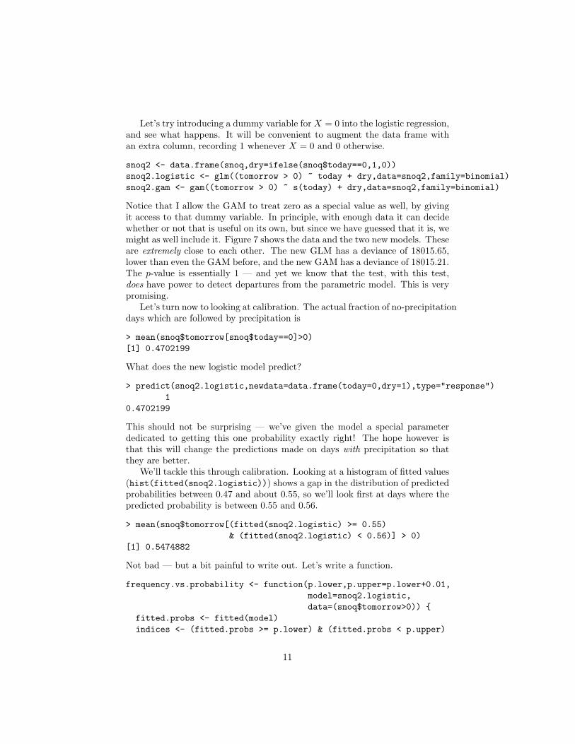
Let’s turn now to looking at calibration. The actual fraction of no-precipitationdays which are followed by precipitation is

> mean(snoq$tomorrow[snoq$today==0]>0)[1] 0.4702199

What does the new logistic model predict?

> predict(snoq2.logistic,newdata=data.frame(today=0,dry=1),type="response")1

0.4702199

This should not be surprising — we’ve given the model a special parameterdedicated to getting this one probability exactly right! The hope however isthat this will change the predictions made on days with precipitation so thatthey are better.

We’ll tackle this through calibration. Looking at a histogram of fitted values(hist(fitted(snoq2.logistic))) shows a gap in the distribution of predictedprobabilities between 0.47 and about 0.55, so we’ll look first at days where thepredicted probability is between 0.55 and 0.56.

> mean(snoq$tomorrow[(fitted(snoq2.logistic) >= 0.55)& (fitted(snoq2.logistic) < 0.56)] > 0)

[1] 0.5474882

Not bad — but a bit painful to write out. Let’s write a function.

frequency.vs.probability <- function(p.lower,p.upper=p.lower+0.01,model=snoq2.logistic,data=(snoq$tomorrow>0)) {

fitted.probs <- fitted(model)indices <- (fitted.probs >= p.lower) & (fitted.probs < p.upper)

11

0 100 200 300 400

0.0

0.2

0.4

0.6

0.8

1.0

Precipitation today (1/100 inch)

Pos

itive

pre

cipi

tatio

n to

mor

row

?

plot((tomorrow>0)~today,data=snoq,xlab="Precipitation today (1/100 inch)",ylab="Positive precipitation tomorrow?")

rug(snoq$today,side=1,col="grey")

data.plot=data.frame(data.plot,dry=ifelse(data.plot$today==0,1,0))logistic.predictions2 <- predict(snoq2.logistic,newdata=data.plot,se.fit=TRUE)lines(0:500,ilogit(logistic.predictions2$fit))lines(0:500,ilogit(logistic.predictions2$fit+1.96*logistic.predictions2$se.fit),

lty=2)lines(0:500,ilogit(logistic.predictions2$fit-1.96*logistic.predictions2$se.fit),

lty=2)gam.predictions2 <- predict.gam(snoq2.gam,newdata=data.plot,se.fit=TRUE)lines(0:500,ilogit(gam.predictions2$fit),col="blue")lines(0:500,ilogit(gam.predictions2$fit+1.96*gam.predictions2$se.fit),

col="blue",lty=2)lines(0:500,ilogit(gam.predictions2$fit-1.96*gam.predictions2$se.fit),

col="blue",lty=2)

Figure 7: As Figure 6, but allowing the two models to use a dummy variableindicating when today is completely dry (X = 0).

12

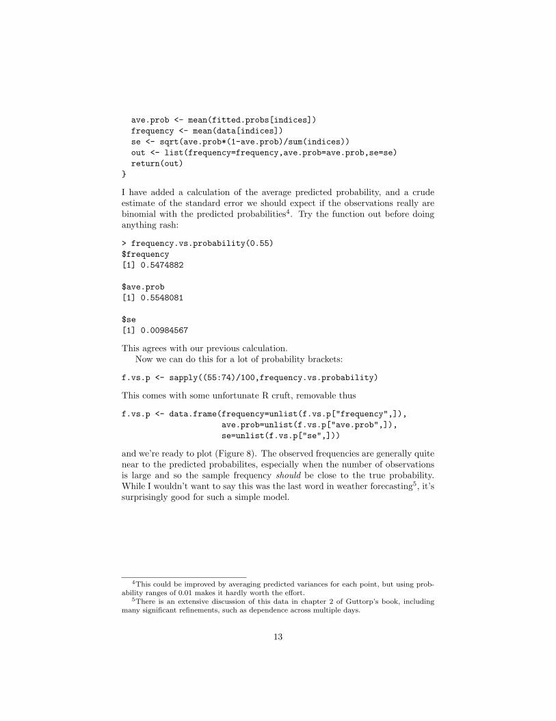
ave.prob <- mean(fitted.probs[indices])frequency <- mean(data[indices])se <- sqrt(ave.prob*(1-ave.prob)/sum(indices))out <- list(frequency=frequency,ave.prob=ave.prob,se=se)return(out)

}

I have added a calculation of the average predicted probability, and a crudeestimate of the standard error we should expect if the observations really arebinomial with the predicted probabilities4. Try the function out before doinganything rash:

> frequency.vs.probability(0.55)$frequency[1] 0.5474882

$ave.prob[1] 0.5548081

$se[1] 0.00984567

This agrees with our previous calculation.Now we can do this for a lot of probability brackets:

f.vs.p <- sapply((55:74)/100,frequency.vs.probability)

This comes with some unfortunate R cruft, removable thus

f.vs.p <- data.frame(frequency=unlist(f.vs.p["frequency",]),ave.prob=unlist(f.vs.p["ave.prob",]),se=unlist(f.vs.p["se",]))

and we’re ready to plot (Figure 8). The observed frequencies are generally quitenear to the predicted probabilites, especially when the number of observationsis large and so the sample frequency should be close to the true probability.While I wouldn’t want to say this was the last word in weather forecasting5, it’ssurprisingly good for such a simple model.

4This could be improved by averaging predicted variances for each point, but using prob-ability ranges of 0.01 makes it hardly worth the effort.

5There is an extensive discussion of this data in chapter 2 of Guttorp’s book, includingmany significant refinements, such as dependence across multiple days.

13

0.0 0.2 0.4 0.6 0.8 1.0

0.0

0.2

0.4

0.6

0.8

1.0

Predicted probabilities

Obs

erve

d fre

quen

cies

plot(f.vs.p$ave.prob,f.vs.p$frequency,xlim=c(0,1),ylim=c(0,1),xlab="Predicted probabilities",ylab="Observed frequencies")

rug(fitted(snoq2.logistic),col="grey")abline(0,1,col="grey")segments(x0=f.vs.p$ave.prob,y0=f.vs.p$ave.prob-1.96*f.vs.p$se,

y1=f.vs.p$ave.prob+1.96*f.vs.p$se)

Figure 8: Calibration plot for the modified logistic regression modelsnoq2.logistic. Points show the actual frequency of precipitation for eachlevel of predicted probability. Vertical lines are (approximate) 95% samplingintervals for the frequency, given the predicted probability and the number ofobservations.

14