15. anova for balanced split-plot experiments among whole-plot-factor marginal means inferences on )
TRANSCRIPT
15. ANOVA for Balanced
Split-Plot Experiments
Copyright c©2018 (Iowa State University) 15. Statistics 510 1 / 47
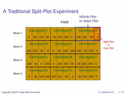
A Traditional Split-Plot Experiment
Field
Block 1
Block 2
Block 3
Block 4 Genotype A Genotype B Genotype C
Genotype A Genotype B Genotype C
Genotype A Genotype B Genotype C
Genotype A Genotype B Genotype C
0 50 100 150 50 0 100 150 150 0 100 50
150 0 100 50 0 100 50 150 100 0 50 150
100 150 50 0 0 50 100 150 50 0 100 150
0 150 50 100 150 0 100 50 50 0 150 100
Whole Plot or Main Plot
Split Plot or
Sub Plot
Copyright c©2018 (Iowa State University) 15. Statistics 510 2 / 47
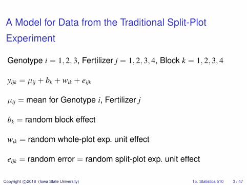
A Model for Data from the Traditional Split-Plot
Experiment
Genotype i = 1, 2, 3, Fertilizer j = 1, 2, 3, 4, Block k = 1, 2, 3, 4
yijk = µij + bk + wik + eijk
µij = mean for Genotype i, Fertilizer j
bk = random block effect
wik = random whole-plot exp. unit effect
eijk = random error = random split-plot exp. unit effect
Copyright c©2018 (Iowa State University) 15. Statistics 510 3 / 47
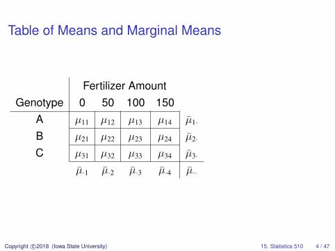
Table of Means and Marginal Means
Fertilizer AmountGenotype 0 50 100 150
A µ11 µ12 µ13 µ14 µ1·
B µ21 µ22 µ23 µ24 µ2·
C µ31 µ32 µ33 µ34 µ3·
µ·1 µ·2 µ·3 µ·4 µ··
Copyright c©2018 (Iowa State University) 15. Statistics 510 4 / 47
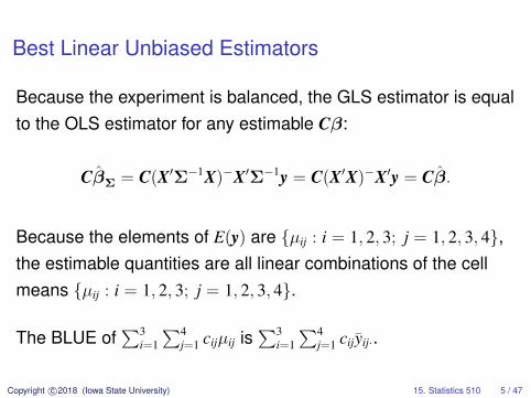
Best Linear Unbiased Estimators
Because the experiment is balanced, the GLS estimator is equalto the OLS estimator for any estimable Cβ:
CβΣ = C(X′Σ−1X)−X′Σ−1y = C(X′X)−X′y = Cβ.
Because the elements of E(y) are {µij : i = 1, 2, 3; j = 1, 2, 3, 4},the estimable quantities are all linear combinations of the cellmeans {µij : i = 1, 2, 3; j = 1, 2, 3, 4}.
The BLUE of∑3
i=1
∑4j=1 cijµij is
∑3i=1
∑4j=1 cijyij·.
Copyright c©2018 (Iowa State University) 15. Statistics 510 5 / 47
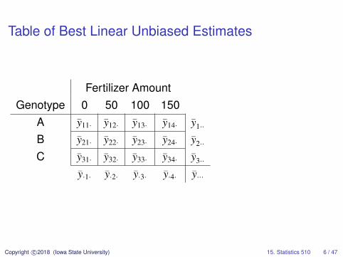
Table of Best Linear Unbiased Estimates
Fertilizer AmountGenotype 0 50 100 150
A y11· y12· y13· y14· y1··
B y21· y22· y23· y24· y2··
C y31· y32· y33· y34· y3··
y·1· y·2· y·3· y·4· y···
Copyright c©2018 (Iowa State University) 15. Statistics 510 6 / 47
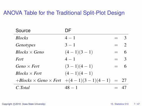
ANOVA Table for the Traditional Split-Plot Design
Source DF
Blocks 4− 1 = 3
Genotypes 3− 1 = 2
Blocks× Geno (4− 1)(3− 1) = 6
Fert 4− 1 = 3
Geno× Fert (3− 1)(4− 1) = 6
Blocks× Fert (4− 1)(4− 1)
+Blocks× Geno× Fert +(4− 1)(3− 1)(4− 1) = 27
C.Total 48− 1 = 47
Copyright c©2018 (Iowa State University) 15. Statistics 510 7 / 47
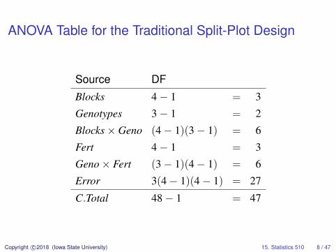
ANOVA Table for the Traditional Split-Plot Design
Source DF
Blocks 4− 1 = 3
Genotypes 3− 1 = 2
Blocks× Geno (4− 1)(3− 1) = 6
Fert 4− 1 = 3
Geno× Fert (3− 1)(4− 1) = 6
Error 3(4− 1)(4− 1) = 27
C.Total 48− 1 = 47
Copyright c©2018 (Iowa State University) 15. Statistics 510 8 / 47
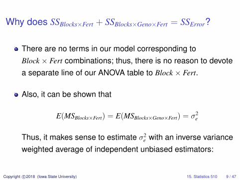
Why does SSBlocks×Fert + SSBlocks×Geno×Fert = SSError?
There are no terms in our model corresponding toBlock × Fert combinations; thus, there is no reason to devotea separate line of our ANOVA table to Block × Fert.
Also, it can be shown that
E(MSBlocks×Fert) = E(MSBlocks×Geno×Fert) = σ2e
Thus, it makes sense to estimate σ2e with an inverse variance
weighted average of independent unbiased estimators:
Copyright c©2018 (Iowa State University) 15. Statistics 510 9 / 47
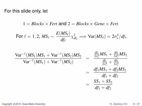
For this slide only, let
1 = Blocks× Fert and 2 = Blocks× Geno× Fert.
For ` = 1, 2, MS` ∼E(MS`)
df`χ2
df` =⇒ Var(MS`) = 2σ4e/df`.
Var−1(MS1)MS1 + Var−1(MS2)MS2
Var−1(MS1) + Var−1(MS2)=
df12σ4
eMS1 + df2
2σ4eMS2
df12σ4
e+ df2
2σ4e
=df1MS1 + df2MS2
df1 + df2
=SS1 + SS2
df1 + df2
Copyright c©2018 (Iowa State University) 15. Statistics 510 10 / 47
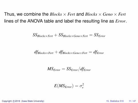
Thus, we combine the Blocks× Fert and Blocks× Geno× Fert
lines of the ANOVA table and label the resulting line as Error.
SSBlocks×Fert + SSBlocks×Geno×Fert = SSError
dfBlocks×Fert + dfBlocks×Geno×Fert = dfError
MSError = SSError/dfError
E(MSError) = σ2e
Copyright c©2018 (Iowa State University) 15. Statistics 510 11 / 47
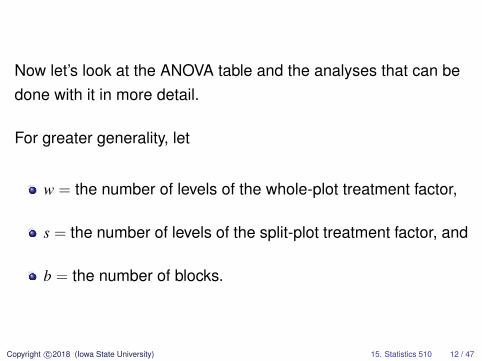
Now let’s look at the ANOVA table and the analyses that can bedone with it in more detail.
For greater generality, let
w = the number of levels of the whole-plot treatment factor,
s = the number of levels of the split-plot treatment factor, and
b = the number of blocks.
Copyright c©2018 (Iowa State University) 15. Statistics 510 12 / 47
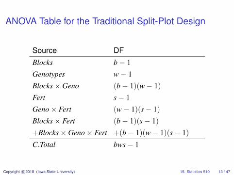
ANOVA Table for the Traditional Split-Plot Design
Source DF
Blocks b− 1
Genotypes w− 1
Blocks× Geno (b− 1)(w− 1)
Fert s− 1
Geno× Fert (w− 1)(s− 1)
Blocks× Fert (b− 1)(s− 1)
+Blocks× Geno× Fert +(b− 1)(w− 1)(s− 1)
C.Total bws− 1
Copyright c©2018 (Iowa State University) 15. Statistics 510 13 / 47

ANOVA Table for the Traditional Split-Plot Design
Source DF
Blocks b− 1
Genotypes w− 1
Blocks× Geno (b− 1)(w− 1)
Fert s− 1
Geno× Fert (w− 1)(s− 1)
Error w(b− 1)(s− 1)
C.Total bws− 1
Copyright c©2018 (Iowa State University) 15. Statistics 510 14 / 47
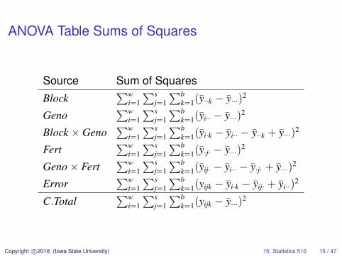
ANOVA Table Sums of Squares
Source Sum of Squares
Block∑w
i=1
∑sj=1
∑bk=1(y··k − y···)2
Geno∑w
i=1
∑sj=1
∑bk=1(yi·· − y···)2
Block × Geno∑w
i=1
∑sj=1
∑bk=1(yi·k − yi·· − y··k + y···)2
Fert∑w
i=1
∑sj=1
∑bk=1(y·j· − y···)2
Geno× Fert∑w
i=1
∑sj=1
∑bk=1(yij· − yi·· − y·j· + y···)2
Error∑w
i=1
∑sj=1
∑bk=1(yijk − yi·k − yij· + yi··)
2
C.Total∑w
i=1
∑sj=1
∑bk=1(yijk − y···)2
Copyright c©2018 (Iowa State University) 15. Statistics 510 15 / 47
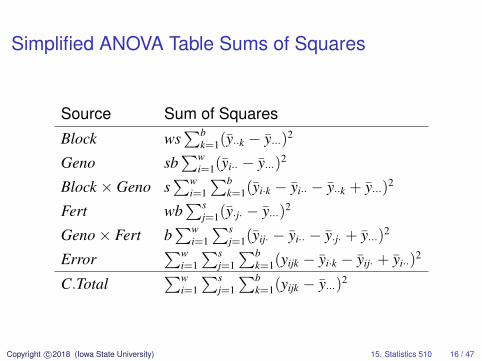
Simplified ANOVA Table Sums of Squares
Source Sum of Squares
Block ws∑b
k=1(y··k − y···)2
Geno sb∑w
i=1(yi·· − y···)2
Block × Geno s∑w
i=1
∑bk=1(yi·k − yi·· − y··k + y···)2
Fert wb∑s
j=1(y·j· − y···)2
Geno× Fert b∑w
i=1
∑sj=1(yij· − yi·· − y·j· + y···)2
Error∑w
i=1
∑sj=1
∑bk=1(yijk − yi·k − yij· + yi··)
2
C.Total∑w
i=1
∑sj=1
∑bk=1(yijk − y···)2
Copyright c©2018 (Iowa State University) 15. Statistics 510 16 / 47

E(MSGeno) =sb
w− 1
w∑i=1
E(yi·· − y···)2
=sb
w− 1
w∑i=1
E(µi· − µ·· + wi· − w·· + ei·· − e···)2
= sb{∑w
i=1(µi· − µ··)2
w− 1+ E
[∑wi=1(wi· − w··)2
w− 1
]+ E
[∑wi=1(ei·· − e···)2
w− 1
]}
= sb∑w
i=1(µi· − µ··)2
w− 1+ sb
σ2w
b+ sb
σ2e
sb
= sb∑w
i=1(µi· − µ··)2
w− 1+ sσ2
w + σ2e
Copyright c©2018 (Iowa State University) 15. Statistics 510 17 / 47
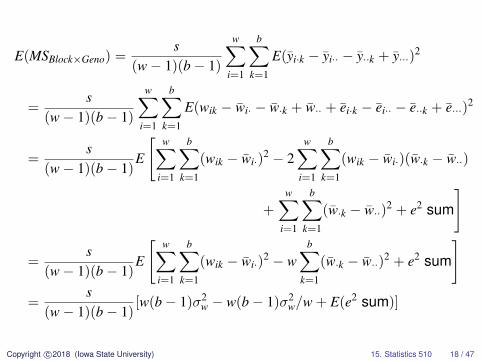
E(MSBlock×Geno) =s
(w− 1)(b− 1)
w∑i=1
b∑k=1
E(yi·k − yi·· − y··k + y···)2
=s
(w− 1)(b− 1)
w∑i=1
b∑k=1
E(wik − wi· − w·k + w·· + ei·k − ei·· − e··k + e···)2
=s
(w− 1)(b− 1)E
[w∑
i=1
b∑k=1
(wik − wi·)2 − 2
w∑i=1
b∑k=1
(wik − wi·)(w·k − w··)
+
w∑i=1
b∑k=1
(w·k − w··)2 + e2 sum
]
=s
(w− 1)(b− 1)E
[w∑
i=1
b∑k=1
(wik − wi·)2 − w
b∑k=1
(w·k − w··)2 + e2 sum
]=
s(w− 1)(b− 1)
[w(b− 1)σ2w − w(b− 1)σ2
w/w + E(e2 sum)]
Copyright c©2018 (Iowa State University) 15. Statistics 510 18 / 47
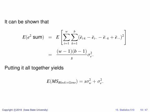
It can be shown that
E(e2 sum) = E
[w∑
i=1
b∑k=1
(ei·k − ei·· − e··k + e···)2
]
=(w− 1)(b− 1)
sσ2
e .
Putting it all together yields
E(MSBlock×Geno) = sσ2w + σ2
e .
Copyright c©2018 (Iowa State University) 15. Statistics 510 19 / 47
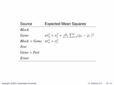
Source Expected Mean Squares
Block
Geno sσ2w + σ2
e + sbw−1
∑wi=1(µi· − µ··)2
Block × Geno sσ2w + σ2
e
Fert
Geno× Fert
Error
Copyright c©2018 (Iowa State University) 15. Statistics 510 20 / 47
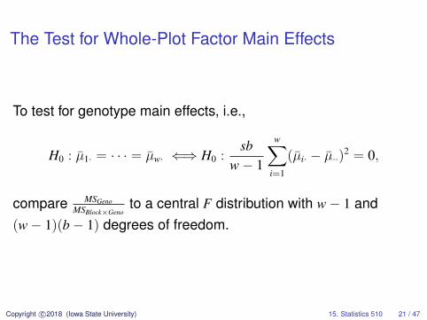
The Test for Whole-Plot Factor Main Effects
To test for genotype main effects, i.e.,
H0 : µ1· = · · · = µw· ⇐⇒ H0 :sb
w− 1
w∑i=1
(µi· − µ··)2 = 0,
compare MSGenoMSBlock×Geno
to a central F distribution with w− 1 and(w− 1)(b− 1) degrees of freedom.
Copyright c©2018 (Iowa State University) 15. Statistics 510 21 / 47
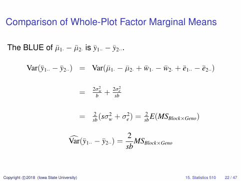
Comparison of Whole-Plot Factor Marginal Means
The BLUE of µ1· − µ2· is y1·· − y2··.
Var(y1·· − y2··) = Var(µ1· − µ2· + w1· − w2· + e1·· − e2··)
= 2σ2w
b + 2σ2e
sb
= 2sb(sσ2
w + σ2e ) = 2
sbE(MSBlock×Geno)
Var(y1·· − y2··) =2sb
MSBlock×Geno
Copyright c©2018 (Iowa State University) 15. Statistics 510 22 / 47

We can use
t =y1·· − y2·· − (µ1· − µ2·)√
2sbMSBlock×Geno
∼ t(w−1)(b−1)
to get tests of H0 : µ1· = µ2·
or construct confidence intervals for µ1· − µ2·.
Copyright c©2018 (Iowa State University) 15. Statistics 510 23 / 47
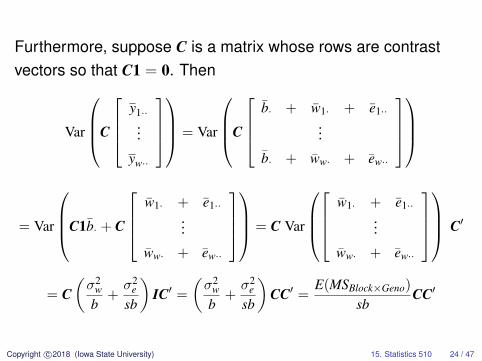
Furthermore, suppose C is a matrix whose rows are contrastvectors so that C1 = 0. Then
Var
C
y1··...
yw··
= Var
C
b· + w1· + e1··
...
b· + ww· + ew··
= Var
C1b· + C
w1· + e1··
...
ww· + ew··
= C Var
w1· + e1··...
ww· + ew··
C′
= C(σ2
w
b+σ2
e
sb
)IC′ =
(σ2
w
b+σ2
e
sb
)CC′ =
E(MSBlock×Geno)
sbCC′
Copyright c©2018 (Iowa State University) 15. Statistics 510 24 / 47
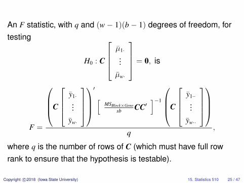
An F statistic, with q and (w− 1)(b− 1) degrees of freedom, fortesting
H0 : C
µ1·...µw·
= 0, is
F =
C
y1·...
yw·
′ [
MSBlock×Genosb CC′
]−1
C
y1··...
yw··
q,
where q is the number of rows of C (which must have full rowrank to ensure that the hypothesis is testable).
Copyright c©2018 (Iowa State University) 15. Statistics 510 25 / 47
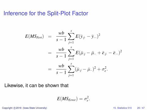
Inference for the Split-Plot Factor
E(MSFert) =wb
s− 1
s∑j=1
E(y·j· − y···)2
=wb
s− 1
s∑j=1
E(µ·j − µ·· + e·j· − e···)2
=wb
s− 1
s∑j=1
(µ·j − µ··)2 + σ2e .
Likewise, it can be shown that
E(MSError) = σ2e .
Copyright c©2018 (Iowa State University) 15. Statistics 510 26 / 47
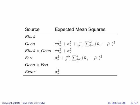
Source Expected Mean Squares
Block
Geno sσ2w + σ2
e + sbw−1
∑wi=1(µi· − µ··)2
Block × Geno sσ2w + σ2
e
Fert σ2e + wb
s−1
∑sj=1(µ·j − µ··)2
Geno× Fert
Error σ2e
Copyright c©2018 (Iowa State University) 15. Statistics 510 27 / 47

The Test for Split-Plot Factor Main Effects
To test for fertilizer main effects, i.e.,
H0 : µ·1 = · · · = µ·s ⇐⇒ H0 :wb
s− 1
s∑j=1
(µ·j − µ··)2 = 0,
compare MSFertMSError
to a central F distribution with s− 1 andw(s− 1)(b− 1) degrees of freedom.
Copyright c©2018 (Iowa State University) 15. Statistics 510 28 / 47
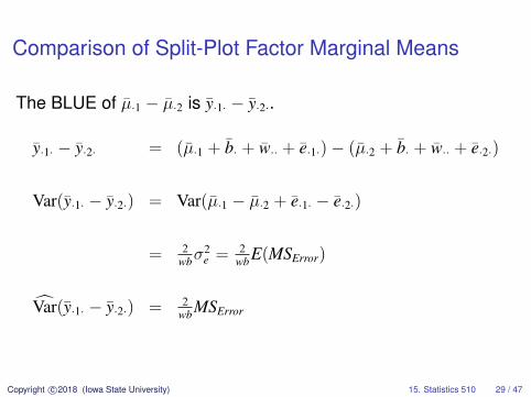
Comparison of Split-Plot Factor Marginal Means
The BLUE of µ·1 − µ·2 is y·1· − y·2·.
y·1· − y·2· = (µ·1 + b· + w·· + e·1·)− (µ·2 + b· + w·· + e·2·)
Var(y·1· − y·2·) = Var(µ·1 − µ·2 + e·1· − e·2·)
= 2wbσ
2e = 2
wbE(MSError)
Var(y·1· − y·2·) = 2wbMSError
Copyright c©2018 (Iowa State University) 15. Statistics 510 29 / 47

We can use
t =y·1· − y·2· − (µ·1 − µ·2)√
2wbMSError
∼ tw(s−1)(b−1)
to get tests of H0 : µ·1 = µ·2
or to construct confidence intervals for µ·1 − µ·2.
Copyright c©2018 (Iowa State University) 15. Statistics 510 30 / 47
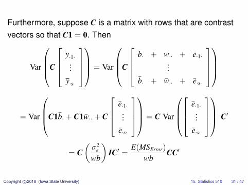
Furthermore, suppose C is a matrix with rows that are contrastvectors so that C1 = 0. Then
Var
C
y·1·...
y·s·
= Var
C
b· + w·· + e·1·
...b· + w·· + e·s·
= Var
C1b· + C1w·· + C
e·1·...
e·s·
= C Var
e·1·...
e·s·
C′
= C(σ2
e
wb
)IC′ =
E(MSError)
wbCC′
Copyright c©2018 (Iowa State University) 15. Statistics 510 31 / 47
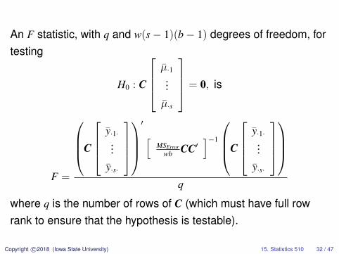
An F statistic, with q and w(s− 1)(b− 1) degrees of freedom, fortesting
H0 : C
µ·1...µ·s
= 0, is
F =
C
y·1·...
y·s·
′ [
MSErrorwb CC′
]−1
C
y·1·...
y·s·
q
where q is the number of rows of C (which must have full rowrank to ensure that the hypothesis is testable).
Copyright c©2018 (Iowa State University) 15. Statistics 510 32 / 47
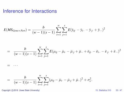
Inference for Interactions
E(MSGeno×Fert) =b
(w− 1)(s− 1)
w∑i=1
s∑j=1
E(yij· − yi·· − y·j· + y···)2
=b
(w− 1)(s− 1)
w∑i=1
s∑j=1
E(µij − µi· − µ·j + µ·· + eij· − ei·· − e·j· + e···)2
= · · ·
=b
(w− 1)(s− 1)
w∑i=1
s∑j=1
(µij − µi· − µ·j + µ··)2 + σ2
e .
Copyright c©2018 (Iowa State University) 15. Statistics 510 33 / 47
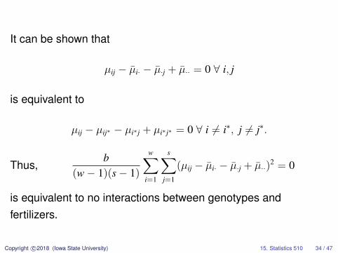
It can be shown that
µij − µi· − µ·j + µ·· = 0 ∀ i, j
is equivalent to
µij − µij∗ − µi∗j + µi∗j∗ = 0 ∀ i 6= i∗, j 6= j∗.
Thus,b
(w− 1)(s− 1)
w∑i=1
s∑j=1
(µij − µi· − µ·j + µ··)2 = 0
is equivalent to no interactions between genotypes andfertilizers.
Copyright c©2018 (Iowa State University) 15. Statistics 510 34 / 47
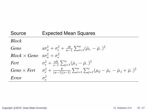
Source Expected Mean Squares
Block
Geno sσ2w + σ2
e + sbw−1
∑wi=1(µi· − µ··)2
Block × Geno sσ2w + σ2
e
Fert σ2e + wb
s−1
∑sj=1(µ·j − µ··)2
Geno× Fert σ2e + b
(w−1)(s−1)
∑wi=1
∑sj=1(µij − µi· − µ·j + µ··)
2
Error σ2e
Copyright c©2018 (Iowa State University) 15. Statistics 510 35 / 47
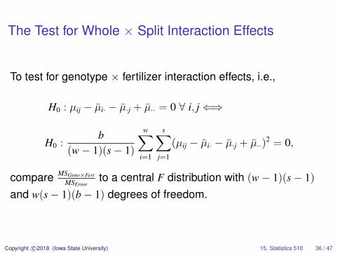
The Test for Whole × Split Interaction Effects
To test for genotype × fertilizer interaction effects, i.e.,
H0 : µij − µi· − µ·j + µ·· = 0 ∀ i, j⇐⇒
H0 :b
(w− 1)(s− 1)
w∑i=1
s∑j=1
(µij − µi· − µ·j + µ··)2 = 0,
compare MSGeno×FertMSError
to a central F distribution with (w− 1)(s− 1)
and w(s− 1)(b− 1) degrees of freedom.
Copyright c©2018 (Iowa State University) 15. Statistics 510 36 / 47
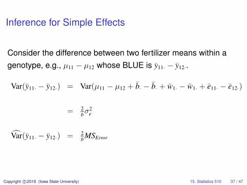
Inference for Simple Effects
Consider the difference between two fertilizer means within agenotype, e.g., µ11 − µ12 whose BLUE is y11· − y12·.
Var(y11· − y12·) = Var(µ11 − µ12 + b· − b· + w1· − w1· + e11· − e12·)
= 2bσ
2e
Var(y11· − y12·) = 2bMSError
Copyright c©2018 (Iowa State University) 15. Statistics 510 37 / 47

We can use
t =y11· − y12· − (µ11 − µ12)√
2bMSError
∼ tw(s−1)(b−1)
to get tests of H0 : µ11 = µ12
or construct confidence intervals for µ11 − µ12.
Copyright c©2018 (Iowa State University) 15. Statistics 510 38 / 47
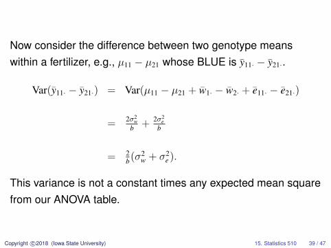
Now consider the difference between two genotype meanswithin a fertilizer, e.g., µ11 − µ21 whose BLUE is y11· − y21·.
Var(y11· − y21·) = Var(µ11 − µ21 + w1· − w2· + e11· − e21·)
= 2σ2w
b + 2σ2e
b
= 2b(σ2
w + σ2e ).
This variance is not a constant times any expected mean squarefrom our ANOVA table.
Copyright c©2018 (Iowa State University) 15. Statistics 510 39 / 47
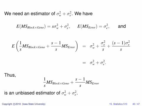
We need an estimator of σ2w + σ2
e . We have
E(MSBlock×Geno) = sσ2w + σ2
e , E(MSError) = σ2e , and
E(
1s
MSBlock×Geno +s− 1
sMSError
)= σ2
w +σ2
e
s+
(s− 1)σ2e
s
= σ2w + σ2
e .
Thus,1s
MSBlock×Geno +s− 1
sMSError
is an unbiased estimator of σ2w + σ2
e .
Copyright c©2018 (Iowa State University) 15. Statistics 510 40 / 47
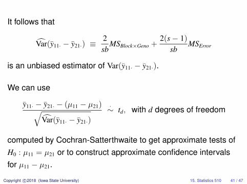
It follows that
Var(y11· − y21·) ≡2sb
MSBlock×Geno +2(s− 1)
sbMSError
is an unbiased estimator of Var(y11· − y21·).
We can use
y11· − y21· − (µ11 − µ21)√Var(y11· − y21·)
·∼ td, with d degrees of freedom
computed by Cochran-Satterthwaite to get approximate tests ofH0 : µ11 = µ21 or to construct approximate confidence intervalsfor µ11 − µ21.
Copyright c©2018 (Iowa State University) 15. Statistics 510 41 / 47
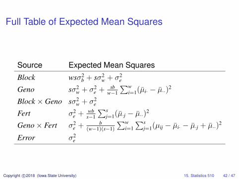
Full Table of Expected Mean Squares
Source Expected Mean Squares
Block wsσ2b + sσ2
w + σ2e
Geno sσ2w + σ2
e + sbw−1
∑wi=1(µi· − µ··)2
Block × Geno sσ2w + σ2
e
Fert σ2e + wb
s−1
∑sj=1(µ·j − µ··)2
Geno× Fert σ2e + b
(w−1)(s−1)
∑wi=1
∑sj=1(µij − µi· − µ·j + µ··)
2
Error σ2e
Copyright c©2018 (Iowa State University) 15. Statistics 510 42 / 47
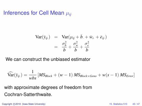
Inferences for Cell Mean µij
Var(yij·) = Var(µij + b· + wi· + eij·)
=σ2
b
b+σ2
w
b+σ2
e
b
We can construct the unbiased estimator
Var(yij·) =1
wbs[MSBlock + (w− 1) MSBlock×Geno + w(s− 1) MSError]
with approximate degrees of freedom fromCochran-Satterthwaite.
Copyright c©2018 (Iowa State University) 15. Statistics 510 43 / 47
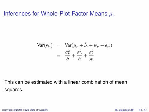
Inferences for Whole-Plot-Factor Means µi·
Var(yi··) = Var(µi· + b· + wi· + ei··)
=σ2
b
b+σ2
w
b+σ2
e
sb
This can be estimated with a linear combination of meansquares.
Copyright c©2018 (Iowa State University) 15. Statistics 510 44 / 47
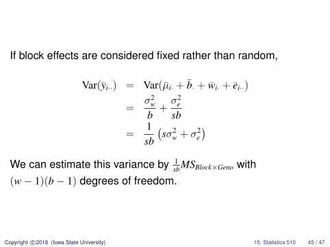
If block effects are considered fixed rather than random,
Var(yi··) = Var(µi· + b· + wi· + ei··)
=σ2
w
b+σ2
e
sb
=1sb
(sσ2
w + σ2e
)We can estimate this variance by 1
sbMSBlock×Geno with(w− 1)(b− 1) degrees of freedom.
Copyright c©2018 (Iowa State University) 15. Statistics 510 45 / 47
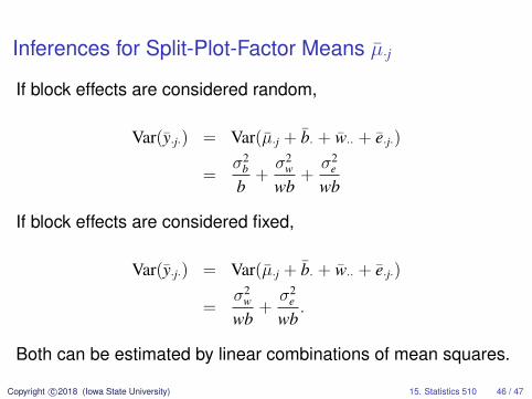
Inferences for Split-Plot-Factor Means µ·j
If block effects are considered random,
Var(y·j·) = Var(µ·j + b· + w·· + e·j·)
=σ2
b
b+σ2
w
wb+σ2
e
wb
If block effects are considered fixed,
Var(y·j·) = Var(µ·j + b· + w·· + e·j·)
=σ2
w
wb+σ2
e
wb.
Both can be estimated by linear combinations of mean squares.
Copyright c©2018 (Iowa State University) 15. Statistics 510 46 / 47
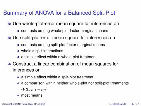
Summary of ANOVA for a Balanced Split-Plot
Use whole-plot-error mean square for inferences oncontrasts among whole-plot-factor marginal means
Use split-plot-error mean square for inferences oncontrasts among split-plot-factor marginal means
whole× split interactions
a simple effect within a whole-plot treatment
Construct a linear combination of mean squares forinferences on
a simple effect within a split-plot treatment
a comparison within neither whole-plot nor split-plot treatments
(e.g., µ11 − µ22)
most means
Copyright c©2018 (Iowa State University) 15. Statistics 510 47 / 47