13-deconvolution corr

8/13/2019 13-Deconvolution CORR

http://slidepdf.com/reader/full/13-deconvolution-corr 1/17

Exercise 13

Deconvolution analysis vs. modelling to document the

process of drug absorptionObjectives

To implement a WNL user model for a monocompartmental model ith to

processes of absorption either ith an algebraic e!uation or ith a set ofdifferential e!uations.

To compare to concurrent models" monocompartmental# ith a single site of

absorption vs. a monocompartmental model ith to sites of absorption using the $%& criterion

To obtain the input function of a drug using deconvolution to reveal informationabout its process of absorption.

Overview

Double pea's in the plasma concentration(time profile folloing oral administrationhave been reported for several compounds. )ultiple pea's after oral administrationof a drug could have several physiological causes.To describe a complicated drug plasma profile li'e a double pea'# there are topossible approaches" *i+ curve fitting using a modified customary compartmentalmodel *ii+ numerical deconvolution to identify the input rate of the drug in the

central compartment.,or the present exercise e ill implement a pharmaco'inetic model in WNL thatas previously used in exercise - *)onte &arlo simulations# ioe!uivalence andithdraal time+ incorporating absorption from to different sites. The results ill becompared ith those from a deconvolution analysis.

Exercise

The goal of this experiment as to compare to formulations *$ and + of a nedrug product administered by the oral route at a dose of 1// 0g'g. Telve *12+animals ere investigated folloing a crossover design and the ra data are givenin the corresponding Excel sheet.

$fter importing the data set in WNL# you ill inspect individual curves# you ill see anirregular initial phase ith a shoulder for some animals *e.g. animal 21+.

1



%t is clear that fitting this animal ith a conventional model ould most li'ely lead tosome misfit especially during the first hours folloing drug administration and even ifa fitting is apparently satisfactory# the estimated parameters could be severelybiased.We ill start to fit these different curves ith a classical monocompartmental model

ith a single rate constant of absorption.

The next figure shos the fitting obtained for animal 21 that loo's rather good.

2



4oever inspection of residuals is more informative and it immediately enablesdeparture to the model to be detected.

&ompute the different parameters associated ith this monocompartmental model.

)onocompartmental model ith a single rate constant of absorption# and meanparameters for the to formulations"

Variable Formulation N Mean SD Min Max CV% Geometric_MeanK10 A 12 0.0418 0.0038 0.0377 0.0490 9.0431 0.0416K10 B 12 0.0371 0.0053 0.0261 0.0447 14.2316 0.0368

V_F A 12 3.1546 0.3450 2.4330 3.5734 10.9365 3.1363V_F B 12 4.1748 1.5003 2.6644 7.8159 35.9374 3.9669K01 A 12 0.0982 0.0140 0.0794 0.1133 14.2178 0.0973K01 B 12 0.1064 0.0121 0.0853 0.1294 11.3558 0.1058

Variable Formulation N Mean SDAUC A 12 766.6596 36.7152AUC B 12 696.0401 123.3195CL_F A 12 0.1307 0.0062CL_F B 12 0.1480 0.0272K01_HL A 12 7.1911 1.0390

K01_HL B 12 6.5905 0.7583Cmax A 12 16.8647 1.0422Cmax B 12 14.7399 3.6567K10_HL A 12 16.7088 1.4535K10_HL B 12 19.0709 3.1261Tmax A 12 15.2337 0.7055Tmax B 12 15.2968 0.7617

3



Diagnostic table for the monocompartmental model"

Formulation Item N Mean SDA AIC 12 14.87 27.6988A CORR_(OBS,PR!" 12 0.9936 0.0064A CSS 12 478.1272 64.4449

A !F 12 11.0000 0.0000A S 12 0.6135 0.4739A SBC 12 16.7937 27.6988A SSR 12 6.4052 6.4875A #CSS 12 478.1272 64.4449A #SSR 12 6.4052 6.4875A !"_C#$$_#&S'($)D* 12 +.,,- +.++4B AIC 12 1+.2112 27.2787B CORR_(OBS,PR!" 12 0.9925 0.0074B CSS 12 378.1471 174.8035B !F 12 11.0000 0.0000B S 12 0.5048 0.3756B SBC 12 12.1284 27.2787

B SSR 12 4.2252 4.4506B #CSS 12 378.1471 174.8035B #SSR 12 4.2252 4.4506B #T_CORR_(OBS,PR!" 12 0.9925 0.0074

Corrected sum of squared observations (CSS), weighted corrected sum of squaredobservations (WCSS), sum of squared residuals (SSR), weighted sum of squaredresiduals (WSSR), estimate of residual standard deviation (S) and degrees offreedom (DF), the correlation between observed Y and redicted Y, the weightedcorrelation, and two measures of goodness of fit! the "#ai#e $nformation Criterion("$C) and Schwar% &a'esian Criterion (S&C)

)odel ith to sites of absorption

We ant to compare results obtained ith this classical model ith those of a usermodel able to describe the same data but ith a model incorporating to sites ofabsorption.This is the model that e previously used to simulate our data set ith &rystal all*exercise -+.

%n this monocompartmental model# a first fraction *,1+ of the administered dose isavailable from site1 ith a rate constant of absorption 5a16 and the second fraction*,2+ of the administered dose is available from site 2 ith a rate constant 5a2. Weassumed that the availability is total and that ,271,16 8c is the volume ofdistribution of the central compartment6This model can describe a double pea' in plasma concentrationtime curves"

9



,raction 1 *:+

,raction 2 *:+

;lasma

8c

5a1

5a2

51/

,1 x Dose

,2 x Dose

,raction 1 *:+

,raction 2 *:+

;lasma

8c

5a1

5a2

51/

,1 x Dose

,2 x Dose

The system can be very easily described by a set of differential e!uations such as"D<*1+ 7 5a1=<*1+D<*2+ 7 5a2=<*2+D<*3+ 7 5a1=<*1+>5a2=<*2+51/=<*3+Where"

D<*1+ 7 5a1=<*1+ is the differential e!uation describing the disappearing of the

drug from the first site of absorption *<*1++ throughout 5a1# a first order rateconstant of absorption#

D<*2+ 7 5a2=<*2+ is the differential e!uation describing the disappearing of the

drug from the second site of absorption *<*2++ throughout 5a2# a first order rate

constant of absorption. ,or both e!uations# the minus sign indicates that the drugdisappears from their respective sites of administration.

D<*3+ 7 5a1=<*1+>5a2=<*2+51/=<*3+ is the differential e!uation describing the

arrival of drug in the central compartment *<3+ ie *5a1=<*1+>5a2=<*2++ minus itsdisappearance from the central compartment ie *51/=<*3++ throughout 51/# thefirst order rate constant of elimination.

$ny ;5 model can be described li'e that ith a rather natural description of the drugdisposition.The next step to describe the model is to !ualify the socall initial condition of thesystem to tell the numerical solver ho to proceed at time /6 here e 'no that afraction of the dose *noted ,?+ is in the first site of absorption and the rest of the

dose *noted 1,?+ in the other site thus"<*1+ 7 ,?=Dose<*2+ 7 *1,?+=Dose<*3+ 7 /Where"

<*1+ 7 ,?=Dose indicates that a ,? fraction of the dose *from / to 1+ is located in

site 1# i.e. *<1+ at time /

<*2+ 7 *1,?+=Dose# indicates that the rest of the dose should be located at time /

in the second site of administration# i.e. < *2+

<*3+ 7 / indicates that there is nothing in the central compartment <*3+ at time /

-



The number of parameters to estimate is 9 namely @,?@# @5a1@# @5a2@# and @51/@.

No e have to rite a set of statements to actually implement this model in WNL.

The folloing set of statements corresponds to the 2 site model ritten ith

differential e!uations to be actually run in WNL.

$ command file is made up of bloc's of text# including a model bloc'# and otherbloc's specifying all or most of the information re!uired to run the model.Each user model must begin ith the 'ey ord MODEL. %t can be folloed by anumber to identify the model# such as )ADEL 1. The model ends ith the commandEOM hich indicates the Bend of the model definitionC.

1. Command blockThe WinNonlin commands are a group of commands *in red+ to define values suchas NP!ME"E!# *the number of parameters+. 4ere e have 9 parameters to

estimate. PNME# $%!$& $'a1$& $'a($& $'1)$ indicates the name of the 9 parameters to beestimated *do not forget !uotation mar's to declare your parameters+.The NCON#"N"# command specifies the number of constants to be used in themodel. ,or our model there ill be only 1 constant that is the dose6 this constantmust be initialied via the WinNonlin interface as for a classical model.The NDE!*+"*+E# command tells WinNonlin the number of differential e!uationsin the model *here n73+.The N%,NC"*ON# command specifies the number of different e!uations that haveobservations associated ith them6 here e declared 3 because if % ish to simulatemy 3 compartments *2 sites of absorption plus the central compartment+# WNLshould solve 3 functions. END bloc' allos WinNonlin commands to be associated ith a model. ,olloing the&A))$ND statement# any WinNonlin command such as N;$?$)ETE?#N&ANT$NT# ;N$)E# etc. may be given. The &A))$ND section concludes ithan END statement.

(. "em-orar variables block8ariables defined in the temporary bloc' are general variables6 that is# they may beused in any bloc'. 4ere % have only one temporary variable *Dose/CON01meaning t2at * can re-lace CON01 in m model b t2e dose 0for e3am-le in t2e

initial condition block.4. #tarting values blockWhen a model is defined by a system of one or more differential e!uations *i.e.NDE!*+"*+E# 4+# the starting values corresponding to each differential e!uation inthe system# must be specified.

5. %unction blockThis group of statements defines the model to be fitted to a set of data. The letter N*here 1# 2 or 3+ denotes the function number. $ function bloc' must appear for eachof the N%,NC"*ON# functions of the command bloc'. The variable , should beassigned to the function value. The function may be"

F



• an algebraic function *e.g. &7Dose8=*'a1=,1=exp*'a1=T+*''a1+ >

'a2=,2=exp*'a2=T+*''a2+ > *'a1=,1=*'a2'+>'a2=,2=*'a1'++=exp*'=T+**'a1'+=*'a2'+++ for our algebraic model

or

• a function of a differential e!uation or differential e!uations defined in one or

more differential bloc's *e.g." ,7<*1+# or ,7 <*1+ etc+

6. Differential e7uation blockThis set of statements is used to define a system of differential e!uations hichdefines a model

M#D)$%ma$& $%ma$& !%)%*+%$- PL T+/a$%ma$& +%* !a/%- 12122009$%ma$& +%* V%$+- 1.0$%ma$& $%ma$&$%ma$& %% m+%*% +mma

C#MMANDS NC#NS"AN" 1 NF0NC"I#NS - ND)$IVA"IV)S - N(A$AM)")$S 4(NAM)S F$' a1' a2' 1+)ND$%ma$& %% /%m+$a$ )a$a*%

")M(#$A$3Doe5C#N1*

)ND $%ma$& %% %$%/a* %:a/+ /a$/; )a*%START<(1" = FR!+%<(2" = (1FR"!+%<(3" = 0>!$%ma$& %% %$%/a* %:a/+

DIFF)$)N"IAD61* 5 a161*D62* 5 a262*D6-* 5 a161*9a262*1+6-*)ND$%ma$& %% a*;%$a /+

F0NC"I#N 1F5 61*)NDF0NC"I#N 2F5 62*)NDF0NC"I#N - F5 6-*)ND$%ma$& %% a %+a$ a$am%/%$

$%ma$& % + m+%*

)#M

G



%f you ant to plot the 3 functions *eg ith a simulation+ you have to edit your dataset indicating the time etc. $lternatively# you can declare only a number of functionse!ual to 1 ie only ,7<*3+.This model using differential e!uations is easy to rite but it is preferable# henever

possible# to use the corresponding algebraic e!uations. %n this case# using theLaplace transform# the e!uation giving the plasma concentration is"

)()( C B AVc

Doset C ++=

With"

)1()110(

11t Ka Exp

Ka K

F Ka A ×−

−

×=

)2()210(

)11(2t Ka Exp

Ka K

F Ka B ×−

−

−×=

( )t K Exp K Ka K Ka

K Ka F Ka K Ka F KaC 10

)102()101(

)101(22)102(11−

−×−

−××+−××=

This model does not exist in the WNL library and e ill implement it.The folloing set of statements corresponds to the 2 site model ritten ith analgebraic e!uation. The structure of the model is the same as for the preceding one6 % Hust add t* as a temorar' variable to tell WNL that the independent variable*alays I+ can be ritten ith a t in my e!uation"

O!L$%ma$& $%ma$& !%)%*+%$- P* /+/a$%ma$& +%* !a/%- 03222011$%ma$& +%* V%$+- 1.0$%ma$& $%ma$&$%ma$& %% m+%*% +mmaCOA>!S>FU>CT?O>S 1>CO> 1>PARATRS 5P>AS @&a1@, @&a2@, @&10@, @V@, @F1@>!$%ma$& %% /%m+$a$ )a$a*%TPORAR!+%=CO>(1"$%ma$&- / /% %%%/ )a$a*%/=>! $%ma$& %% a*;%$a /+FU>CT?O> 1

F= (!+%DV"(((&a1F1%x(&a1/"D(&10&a1"" E (&a2(1F1"%x(&a2/"D(&10&a2"" E (((&a1F1(&a2&10""E(&a2(1F1"(&a1&10"""%x(&10/"D((&a1&10"(&a2&10""""">!$%ma$& %% a %+a$ a$am%/%$$%ma$& % + m+%*

O

J



&reating a ne $&%% model in WNL

elect +ser odel in the )odel Types dialog and clic' -e.t . The $&%% )odelelection dialog appears.

To create this ne Kser )odel# there are to options"

The first option consists of riting your on model ith the assistance of the WNLdialog box that offers a template to edit. To user model templates are providedith WinNonlin" one for models that include only algebraic e!uations and one formodels that include differential e!uations.

The second option consists of selecting one of the to options *differential oralgebraic+ but# instead of riting the hole model yourself# you can copy thepresent ord document and paste it directly in WNL.



?unning the algebraic model corresponding to 2 sites ofabsorption

Ksing the algebraic model# estimate yourself the corresponding parameters for the

29 animals.

Estimate l each individual curve6 loo' at the different graphs including residuals

and then ith the statistical tool of WNL# ma'e the folloing tables.

The first table gives you mean parameters for the 29 animals and the second table isthe diagnostic table provided by WNL and that ill be used to compare the merits ofthe present model against those of the classical monocompartmental model.

)odel ith 2 sites of absorption# mean parameters for the to formulations"

Variable Formulation N Mean SD S) CV% Geometric_Mean

&a1 A 12 0.0543 0.0097 0.0028 17.8621 0.0535&a1 B 12 0.0542 0.0097 0.0028 17.8241 0.0534&a2 A 12 0.0017 0.0004 0.0001 25.2762 0.0016&a2 B 12 0.0018 0.0004 0.0001 24.9447 0.0017F1 A 12 0.6605 0.0694 0.0200 10.5044 0.6570F1 B 12 0.5808 0.1806 0.0521 31.1003 0.5549&10 A 12 0.0815 0.0193 0.0056 23.6972 0.0794&10 B 12 0.0814 0.0194 0.0056 23.8438 0.0793V A 12 1.1852 0.2066 0.0596 17.4331 1.1690V B 12 1.1944 0.2210 0.0638 18.4994 1.1756

Diagnostic table for the model ith 2 sites of absorption"

Formulation

Item N Mean SD Min Max

A A?C 12 42.3582 90.9333 137.2456 47.9836A CORR_(OBS,PR!" 12 0.9939 0.0064 0.9877 1.0000A CSS 12 478.1272 64.4449 414.1760 627.5470A !F 12 9.0000 0.0000 9.0000 9.0000A S 12 0.5761 0.6022 0.0017 1.2943A SBC 12 39.1629 90.9333 134.0503 51.1788A SSR 12 5.9788 6.3681 0.0000 15.0761

A #CSS 12 478.1272 64.4449 414.1760 627.5470A #SSR 12 5.9788 6.3681 0.0000 15.0761A #T_CORR_(OBS,PR!" 12 0.9939 0.0064 0.9877 1.0000B A?C 12 45.4551 85.6979 132.5252 44.3703B CORR_(OBS,PR!" 12 0.9937 0.0066 0.9867 1.0000B CSS 12 378.1471 174.8035 115.9450 670.3750B !F 12 9.0000 0.0000 9.0000 9.0000B S 12 0.4388 0.4728 0.0021 1.1376B SBC 12 42.2598 85.6979 129.3299 47.5656B SSR 12 3.5768 4.2168 0.0000 11.6466B #CSS 12 378.1471 174.8035 115.9450 670.3750B #SSR 12 3.5768 4.2168 0.0000 11.6466B #T_CORR_(OBS,PR!" 12 0.9937 0.0066 0.9867 1.0000

Corrected sum of squared observations (CSS), weighted corrected sum of squaredobservations (WCSS), sum of squared residuals (SSR), weighted sum of squared

1/



residuals (WSSR), estimate of residual standard deviation (S) and degrees offreedom (DF), the correlation between observed Y and redicted Y, the weightedcorrelation, and two measures of goodness of fit! the "#ai#e $nformation Criterion("$C) and Schwar% &a'esian Criterion (S&C)

Com-arison of t2e two concurrent models8

&omparison of the 2 modelling approaches *classical monocompartmental model

against our user model including to phases of absorption+ can be done based ondifferent arguments *goodness of fitting# plot of residuals# and the consideration ofthe $'ai'e %nformation &riterion *$%&++.

$%& is a measure of goodness of fit based on maximum li'elihood. When

comparing several models for a given data set# the model associated ith thesmallest *C is regarded as giving the best fit. $%& is appropriate only forcomparing models that use the same eighting scheme *no eighing here+.

*C / 9N log 0:!## ; (P for modelling in WinNonlin. N is the number of

observations ith positive eight. W? is the eighted residual sum of s!uares.; is the number of parameters that has been estimated.

Muestions"

What are your conclusions

Why is the terminal halflife estimated to be J.-1h */.F3'1/+ hile the classical

monocompartmental model gives an estimate of 1F1 h %s it a flipflopphenomenon

11



Deconvolution analysis

OverviewDeconvolution is primarily used in ;5 to obtain the input function# ie the rate *0gh

or 0g.'g1h+ of drug entry into the central compartment.Deconvolution is useful to reveal in vivo drug release from a given pharmaceuticalform or in our case the delivery from the 2 sites of absorption based on data for a'non drug input *generally an %8 administration+."2e integral of t2e in-ut function gives t2e bioavailabilit.Deconvolution based bioavailability estimation methods are a more general approachto estimate bioavailability than conventional methods since the former provideestimates of both the rate of systemic upta'e and the total systemic dose.Estimated rates of bioavailability may potentially be used to"

• gain insights into the mechanisms of upta'e

•

enable better predictions of bioavailability under varying conditions

Technically# deconvolution is a techni!ue that can be used to estimate an in-utfunction& given the corresponding in-ut9res-onse function 0our data to anal<eand the im-ulse9res-onse function *concentration profile folloing an %8 bolusdose+ for the system.Deconvolution is t2e inverse of convolution.

Literally# if e 'no the disposition curve from a unit %8 dose *bolus+ and the rate ofinput of the drug into the plasma *input rate function+ then e can calculate the

plasma disposition curve from that input by convolution.

12



Deconvolution is the inverse problem# ie to determine the input function from theplasma disposition curve given the unit disposition function# i.e. to determine theinput function f*t+# given the unit impulse response &O*t+ and the input response &*t+.

5ey assumptions for deconvolution are"

1+ linearity" f*D1>D2+ 7 f*D1+ > f*D2+2+ time invariance" f*D+ has the same shape no matter hen D is given.

We ill illustrate these concepts ith our example"

Apen WNL ith our data sheet.

elect Deconvolution from the Tools menu"

The Deconvolution dialog appears!

.

13



Then drag the appropriate variables to the /ime and Concentration fields# dragformulation and animals to the Sort 0ariables field. $ separate analysis is done forevery uni!ue combination of sort variable values.

Enter the dosing units in the Dose units field *here 0g+. The dosing units are used

only hen the input data set has units associated ith the Time and &oncentrationdata *ngmL+. The administered dose as 1//0g'g.

%n the Settings fields# select the number of exponential terms *N+ in the unit

impulse response *here it is 1 because it is a monoexponential model+

Enter the values for $ and alpha in the unit impulse response function *see belo+

The %8 bolus *unit impulse response+ after a 1// 0g'g bolus dose as described bythe folloing e!uation"

)1.0(800)( time Expt C ×−×=

With &*t+ in ngmL thus $7J// ngmL and '1/7/.1 per h ,or this deconvolution# e have to enter a scaled $# ie $1//0g7/.J and alpha is'1/7/.1

elect the setting for Smoothing to be used. "utomatic should be selected if you

ant the program to find the optimal value for the dispersion parameter delta. Thisis the default.

elect the $nitial Change in Rate is 1ero chec' box to constrain the derivative of

the estimated input rate to be ero at the initial time *lag time+.

19



&lic' Calculate. Deconvolution generates a ne chart and or'boo'.Deconvolution generates three charts for each of the sorted 'eys.

The Fitted Curve output plot depicts concentration data from the input data set

plotted against time for animal P21# the curve shos a shoulder in the ascendingphase. This is the deconvoluted curve.

The next figure gives the $nut Rate *0gh+ plot depicting the rate of drug inputagainst time for each profile. 8isual inspection of this figure shos clearly thepresence of to pea's in the input rate describing a rapid and a slo absorptionprocess.

1-



The next figure is the Cumulative $nut plot that displays cumulative drug input *in0gh+ against time for animal 21. 8isual inspection of the curve clearly shos thatthere is a biphasic absorption explaining the initial shoulder seen on the observedcurve.

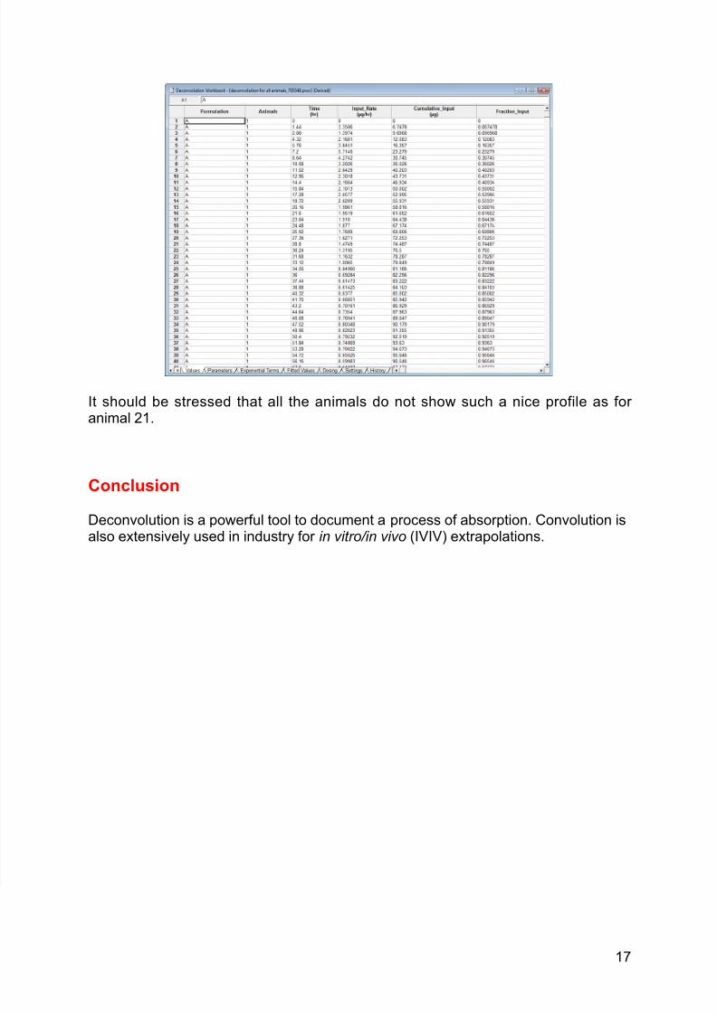
The deconvolution or'boo' contains one or'boo' ith different or'sheets. Thevalues or'sheet includes values for Time# %nput ?ate# &umulative %nput and,raction %nput.

%nspection of the results for animal 1 shos that the total amount of absorbed drugas 1/G 0g'g and that -/: of the drug has been absorbed after a delay of 1-.J9h.

1F



%t should be stressed that all the animals do not sho such a nice profile as foranimal 21.

Conclusion

Deconvolution is a poerful tool to document a process of absorption. &onvolution is

also extensively used in industry for in vitro2in vivo *%8%8+ extrapolations.

1G

13-deconvolution corr

Documents