10/5/2015data mining: concepts and techniques1 chapter 6. classification and prediction what is...
TRANSCRIPT
04/19/23Data Mining: Concepts and Technique
s 1
Chapter 6. Classification and Prediction
What is classification? What
is prediction?
Issues regarding
classification and prediction
Classification by decision
tree induction
Bayesian classification
Rule-based classification
Classification by back
propagation
Support Vector Machines
(SVM)
Associative classification
Lazy learners (or learning
from your neighbors)
Other classification methods
Prediction
Accuracy and error measures
Ensemble methods
Model selection
Summary
04/19/23Data Mining: Concepts and Technique
s 2
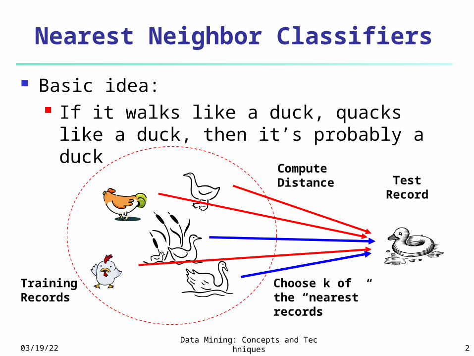
Nearest Neighbor Classifiers
Basic idea: If it walks like a duck, quacks like a duck,
then it’s probably a duck
Training Records
Test Record
Compute Distance
Choose k of the “nearest” records
04/19/23Data Mining: Concepts and Technique
s 3
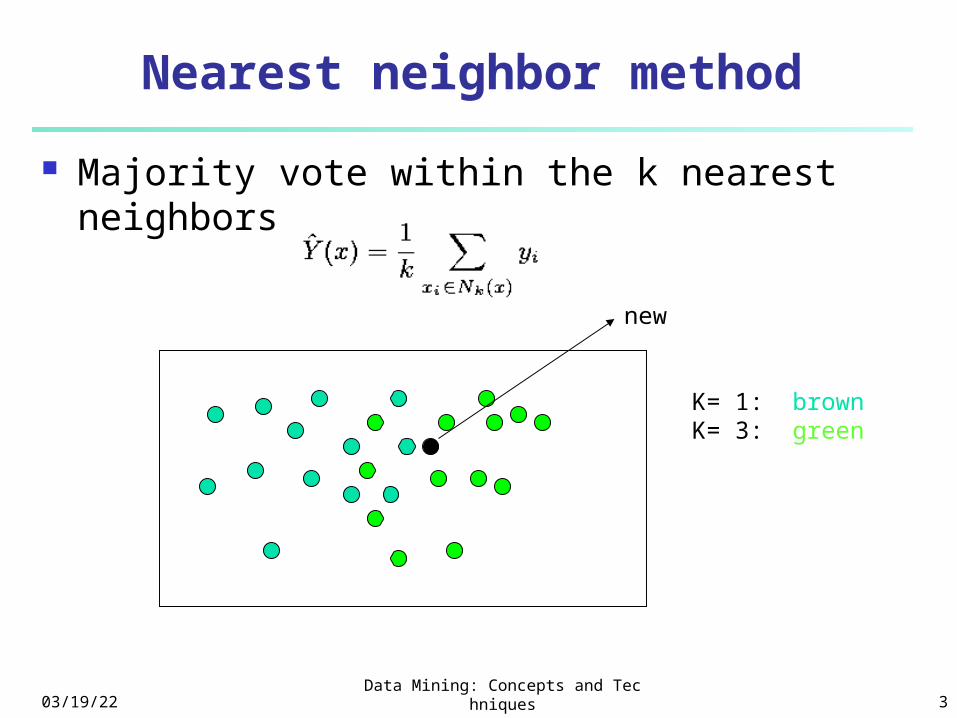
Nearest neighbor method
Majority vote within the k nearest neighbors
K= 1: brownK= 3: green
new
04/19/23Data Mining: Concepts and Technique
s 4
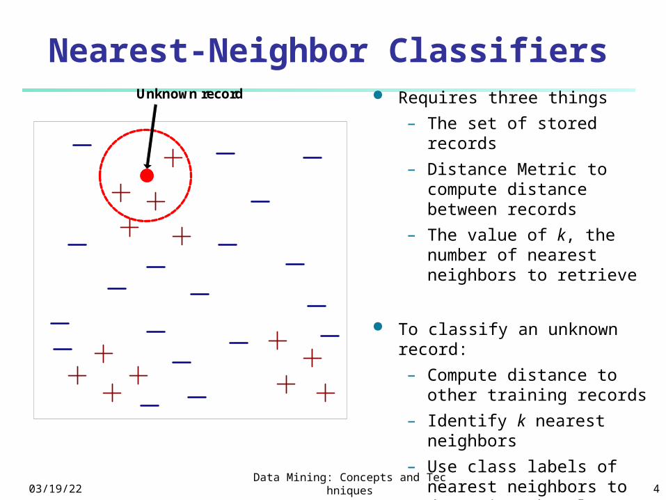
Nearest-Neighbor Classifiers Requires three things
– The set of stored records
– Distance Metric to compute distance between records
– The value of k, the number of nearest neighbors to retrieve
To classify an unknown record:
– Compute distance to other training records
– Identify k nearest neighbors
– Use class labels of nearest neighbors to determine the class label of unknown record (e.g., by taking majority vote)
Unknown record
04/19/23Data Mining: Concepts and Technique
s 5
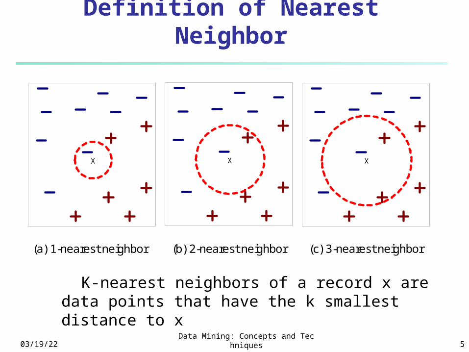
Definition of Nearest Neighbor
X X X
(a) 1-nearest neighbor (b) 2-nearest neighbor (c) 3-nearest neighbor
K-nearest neighbors of a record x are data points that have the k smallest distance to x
04/19/23Data Mining: Concepts and Technique
s 6
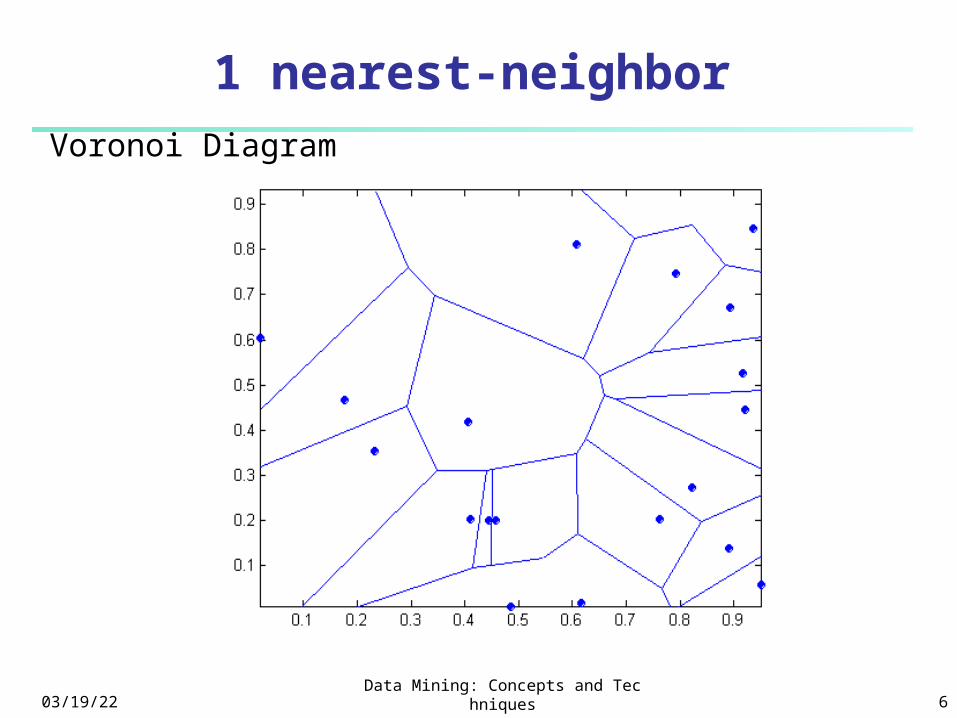
1 nearest-neighborVoronoi Diagram
04/19/23Data Mining: Concepts and Technique
s 7
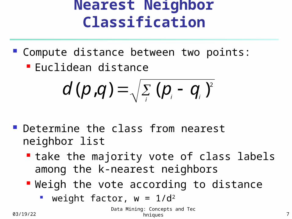
Nearest Neighbor Classification
Compute distance between two points: Euclidean distance
Determine the class from nearest neighbor list take the majority vote of class labels
among the k-nearest neighbors Weigh the vote according to distance
weight factor, w = 1/d2
i ii
qpqpd 2)(),(
04/19/23Data Mining: Concepts and Technique
s 8
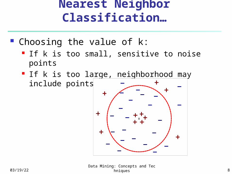
Nearest Neighbor Classification…
Choosing the value of k: If k is too small, sensitive to noise points If k is too large, neighborhood may include
points from other classes
X
04/19/23Data Mining: Concepts and Technique
s 9
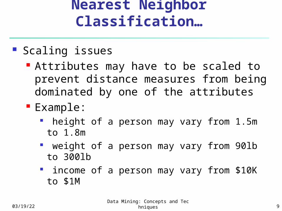
Nearest Neighbor Classification…
Scaling issues Attributes may have to be scaled to
prevent distance measures from being dominated by one of the attributes
Example: height of a person may vary from 1.5m to
1.8m weight of a person may vary from 90lb to
300lb income of a person may vary from $10K to
$1M
04/19/23Data Mining: Concepts and Technique
s 10
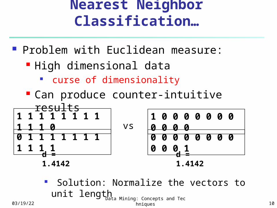
Nearest Neighbor Classification…
Problem with Euclidean measure: High dimensional data
curse of dimensionality Can produce counter-intuitive results
1 1 1 1 1 1 1 1 1 1 1 0
0 1 1 1 1 1 1 1 1 1 1 1
1 0 0 0 0 0 0 0 0 0 0 0
0 0 0 0 0 0 0 0 0 0 0 1vs
d = 1.4142 d = 1.4142
Solution: Normalize the vectors to unit
length
04/19/23Data Mining: Concepts and Technique
s 11
Nearest neighbor Classification…
k-NN classifiers are lazy learners It does not build models explicitly Unlike eager learners such as decision
tree induction and rule-based systems Classifying unknown records are
relatively expensive
04/19/23Data Mining: Concepts and Technique
s 12
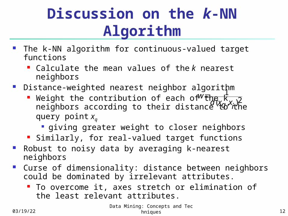
Discussion on the k-NN Algorithm
The k-NN algorithm for continuous-valued target functions Calculate the mean values of the k nearest neighbors
Distance-weighted nearest neighbor algorithm Weight the contribution of each of the k neighbors
according to their distance to the query point xq
giving greater weight to closer neighbors Similarly, for real-valued target functions
Robust to noisy data by averaging k-nearest neighbors Curse of dimensionality: distance between neighbors could
be dominated by irrelevant attributes. To overcome it, axes stretch or elimination of the least
relevant attributes.
wd xq xi
12( , )
04/19/23Data Mining: Concepts and Technique
s 13
Lazy vs. Eager Learning
Lazy vs. eager learning Lazy learning (e.g., instance-based learning): Simply
stores training data (or only minor processing) and waits until it is given a test tuple
Eager learning (the above discussed methods): Given a set of training set, constructs a classification model before receiving new (e.g., test) data to classify
Lazy: less time in training but more time in predicting Accuracy
Lazy method effectively uses a richer hypothesis space since it uses many local linear functions to form its implicit global approximation to the target function
Eager: must commit to a single hypothesis that covers the entire instance space
04/19/23Data Mining: Concepts and Technique
s 14
Lazy Learner: Instance-Based Methods
Instance-based learning: Store training examples and delay the
processing (“lazy evaluation”) until a new instance must be classified
Typical approaches k-nearest neighbor approach
Instances represented as points in a Euclidean space.
Locally weighted regression Constructs local approximation
Case-based reasoning Uses symbolic representations and
knowledge-based inference
04/19/23Data Mining: Concepts and Technique
s 15
Case-Based Reasoning (CBR)
CBR: Uses a database of problem solutions to solve new problems Store symbolic description (tuples or cases)—not points in a Euclidean
space Applications: Customer-service (product-related diagnosis), legal ruling Methodology
Instances represented by rich symbolic descriptions (e.g., function graphs)
Search for similar cases, multiple retrieved cases may be combined Tight coupling between case retrieval, knowledge-based reasoning,
and problem solving Challenges
Find a good similarity metric Indexing based on syntactic similarity measure, and when failure,
backtracking, and adapting to additional cases
04/19/23Data Mining: Concepts and Technique
s 16
Chapter 6. Classification and Prediction
What is classification? What
is prediction?
Issues regarding
classification and prediction
Classification by decision
tree induction
Bayesian classification
Rule-based classification
Classification by back
propagation
Support Vector Machines
(SVM)
Associative classification
Lazy learners (or learning
from your neighbors)
Other classification methods
Prediction
Accuracy and error measures
Ensemble methods
Model selection
Summary
04/19/23Data Mining: Concepts and Technique
s 17
What Is Prediction?
(Numerical) prediction is similar to classification construct a model use model to predict continuous or ordered value for a given
input Prediction is different from classification
Classification refers to predict categorical class label Prediction models continuous-valued functions
Major method for prediction: regression model the relationship between one or more independent or
predictor variables and a dependent or response variable Regression analysis
Linear and multiple regression Non-linear regression Other regression methods: generalized linear model, Poisson
regression, log-linear models, regression trees
04/19/23Data Mining: Concepts and Technique
s 18
Linear Regression
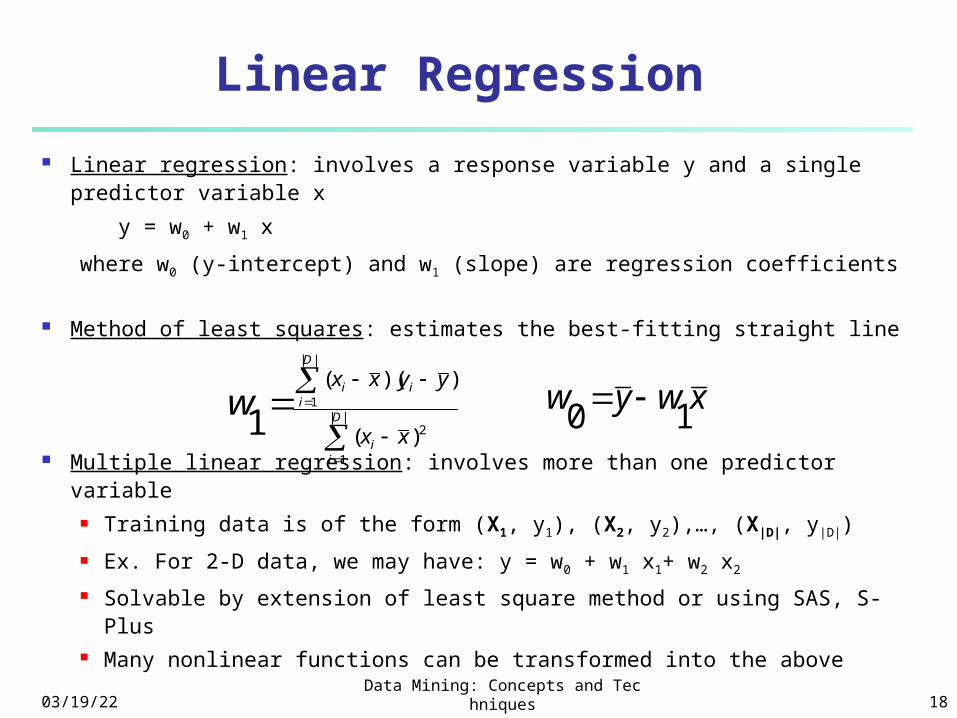
Linear regression: involves a response variable y and a single predictor variable x
y = w0 + w1 x
where w0 (y-intercept) and w1 (slope) are regression coefficients
Method of least squares: estimates the best-fitting straight line
Multiple linear regression: involves more than one predictor variable
Training data is of the form (X1, y1), (X2, y2),…, (X|D|, y|D|)
Ex. For 2-D data, we may have: y = w0 + w1 x1+ w2 x2
Solvable by extension of least square method or using SAS, S-Plus
Many nonlinear functions can be transformed into the above
||
1
2
||
1
)(
))((
1 D
ii
D
iii
xx
yyxxw xwyw
10
04/19/23Data Mining: Concepts and Technique
s 19
Some nonlinear models can be modeled by a polynomial function
A polynomial regression model can be transformed into linear regression model. For example,
y = w0 + w1 x + w2 x2 + w3 x3
convertible to linear with new variables: x2 = x2, x3= x3
y = w0 + w1 x + w2 x2 + w3 x3
Other functions, such as power function, can also be transformed to linear model
Some models are intractable nonlinear (e.g., sum of exponential terms) possible to obtain least square estimates through
extensive calculation on more complex formulae
Nonlinear Regression
04/19/23Data Mining: Concepts and Technique
s 20
Generalized linear model: Foundation on which linear regression can be applied to
modeling categorical response variables Variance of y is a function of the mean value of y, not a
constant Logistic regression: models the prob. of some event
occurring as a linear function of a set of predictor variables Poisson regression: models the data that exhibit a Poisson
distribution Log-linear models: (for categorical data)
Approximate discrete multidimensional prob. distributions Also useful for data compression and smoothing
Regression trees and model trees Trees to predict continuous values rather than class labels
Other Regression-Based Models
04/19/23Data Mining: Concepts and Technique
s 21
Regression Trees and Model Trees
Regression tree: proposed in CART system (Breiman et al. 1984)
CART: Classification And Regression Trees
Each leaf stores a continuous-valued prediction
It is the average value of the predicted attribute for the
training tuples that reach the leaf
Model tree: proposed by Quinlan (1992)
Each leaf holds a regression model—a multivariate linear
equation for the predicted attribute
A more general case than regression tree
Regression and model trees tend to be more accurate than
linear regression when the data are not represented well by a
simple linear model
04/19/23Data Mining: Concepts and Technique
s 22
Predictive modeling: Predict data values or construct generalized linear models based on the database data
One can only predict value ranges or category distributions
Method outline: Minimal generalization Attribute relevance analysis Generalized linear model construction Prediction
Determine the major factors which influence the prediction Data relevance analysis: uncertainty measurement,
entropy analysis, expert judgement, etc. Multi-level prediction: drill-down and roll-up analysis
Predictive Modeling in Multidimensional Databases
04/19/23Data Mining: Concepts and Technique
s 23
Chapter 6. Classification and Prediction
What is classification? What
is prediction?
Issues regarding
classification and prediction
Classification by decision
tree induction
Bayesian classification
Rule-based classification
Classification by back
propagation
Support Vector Machines
(SVM)
Associative classification
Lazy learners (or learning
from your neighbors)
Other classification methods
Prediction
Accuracy and error measures
Ensemble methods
Model selection
Summary
Estimating Error Rates I
Training Error: The proportion of training records that are
misclassified Overly optimistic. Classifiers that overfit the
datasets can have poor accuracy on unseen data
04/19/23 24Data Mining: Concepts and Technique
s
Estimating Error Rates II
Holdout method Partition: Training-and-testing
Given data is randomly partitioned into two independent sets
Training set (e.g., 2/3) for model construction Test set (e.g., 1/3) for accuracy estimation Unbiased, efficient. But require a large number of
samples used for data set with large number of samples
Random sampling: a variation of holdout Repeat holdout k times, accuracy = avg. of the
accuracies obtained
04/19/23 25Data Mining: Concepts and Technique
s
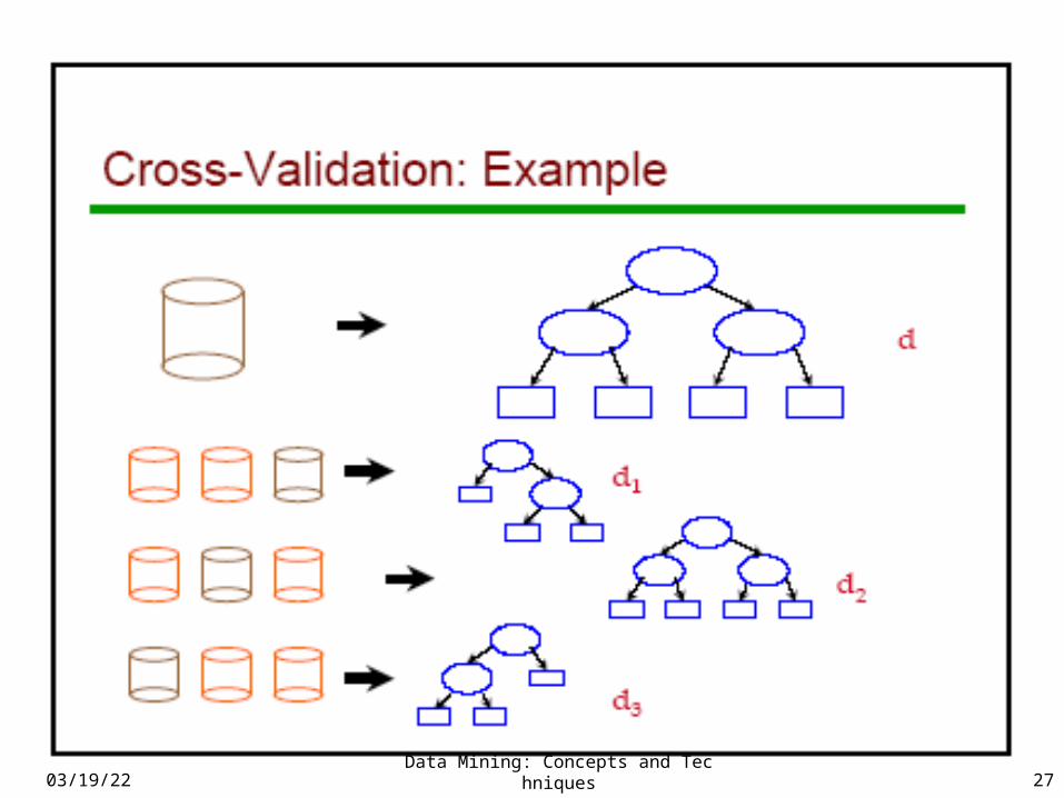
Estimating Error Rates III
Cross-validation (k-fold, where k = 10 is most popular) Randomly partition the data into k mutually
exclusive subsets, each approximately equal size
At i-th iteration, use Di as test set and others as training set
Leave-one-out: k folds where k = # of tuples, for small sized data
Stratified cross-validation: folds are stratified so that class dist. in each fold is approx. the same as that in the initial data
04/19/23 26Data Mining: Concepts and Technique
s
04/19/23 27Data Mining: Concepts and Technique
s
04/19/23 28Data Mining: Concepts and Technique
s
04/19/23Data Mining: Concepts and Technique
s 29
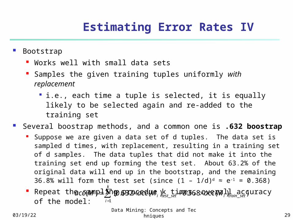
Bootstrap
Works well with small data sets Samples the given training tuples uniformly with replacement
i.e., each time a tuple is selected, it is equally likely to be selected again and re-added to the training set
Several boostrap methods, and a common one is .632 boostrap Suppose we are given a data set of d tuples. The data set is sampled
d times, with replacement, resulting in a training set of d samples. The data tuples that did not make it into the training set end up forming the test set. About 63.2% of the original data will end up in the bootstrap, and the remaining 36.8% will form the test set (since (1 – 1/d)d ≈ e-1 = 0.368)
Repeat the sampling procedue k times, overall accuracy of the model: ))(368.0)(632.0()( _
1_ settraini
k
isettesti MaccMaccMacc
Estimating Error Rates IV
04/19/23Data Mining: Concepts and
Techniques 30
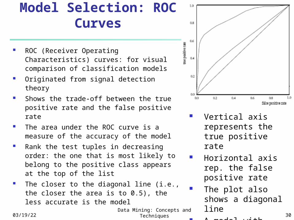
Model Selection: ROC Curves
ROC (Receiver Operating Characteristics) curves: for visual comparison of classification models
Originated from signal detection theory Shows the trade-off between the true
positive rate and the false positive rate The area under the ROC curve is a
measure of the accuracy of the model Rank the test tuples in decreasing
order: the one that is most likely to belong to the positive class appears at the top of the list
The closer to the diagonal line (i.e., the closer the area is to 0.5), the less accurate is the model
Vertical axis represents the true positive rate
Horizontal axis rep. the false positive rate
The plot also shows a diagonal line
A model with perfect accuracy will have an area of 1.0
04/19/23Data Mining: Concepts and Technique
s 31
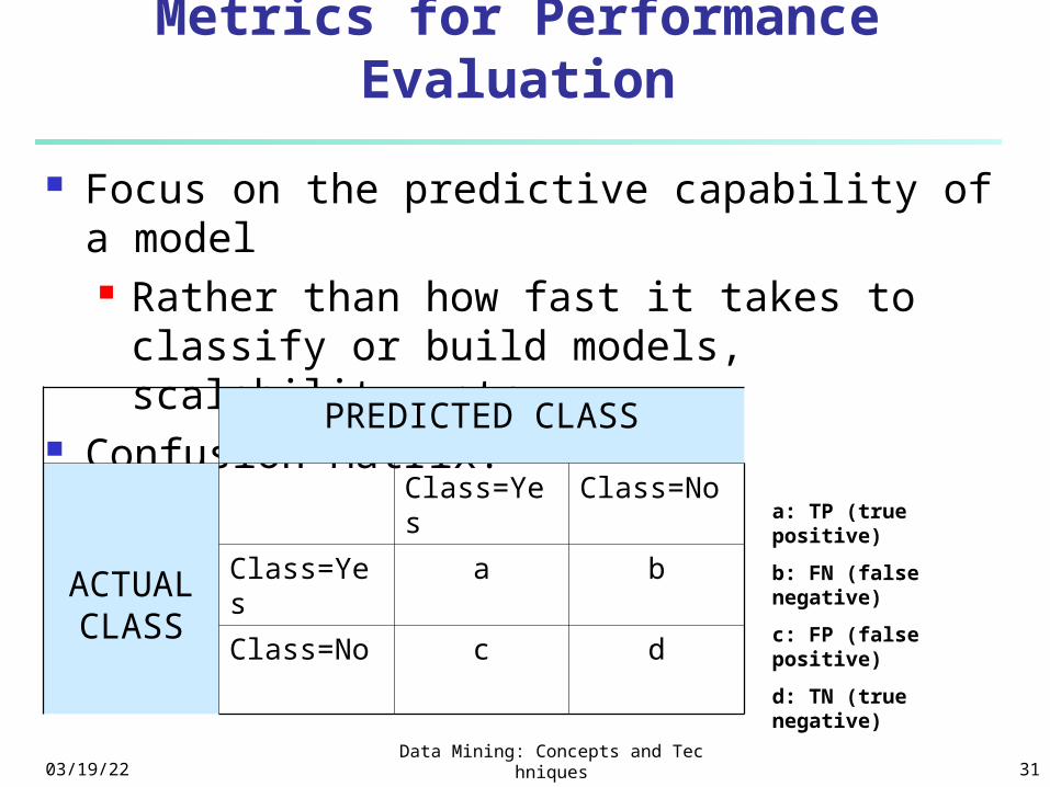
Metrics for Performance Evaluation
Focus on the predictive capability of a model Rather than how fast it takes to classify
or build models, scalability, etc. Confusion Matrix:PREDICTED CLASS
ACTUALCLASS
Class=Yes Class=No
Class=Yes a b
Class=No c d
a: TP (true positive)
b: FN (false negative)
c: FP (false positive)
d: TN (true negative)
04/19/23Data Mining: Concepts and Technique
s 32
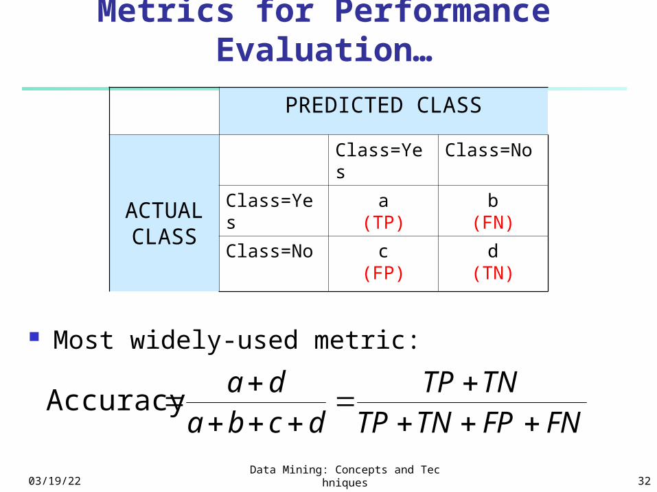
Metrics for Performance Evaluation…
Most widely-used metric:
PREDICTED CLASS
ACTUALCLASS
Class=Yes Class=No
Class=Yes a(TP)
b(FN)
Class=No c(FP)
d(TN)
FNFPTNTPTNTP
dcbada
Accuracy
04/19/23Data Mining: Concepts and Technique
s 33
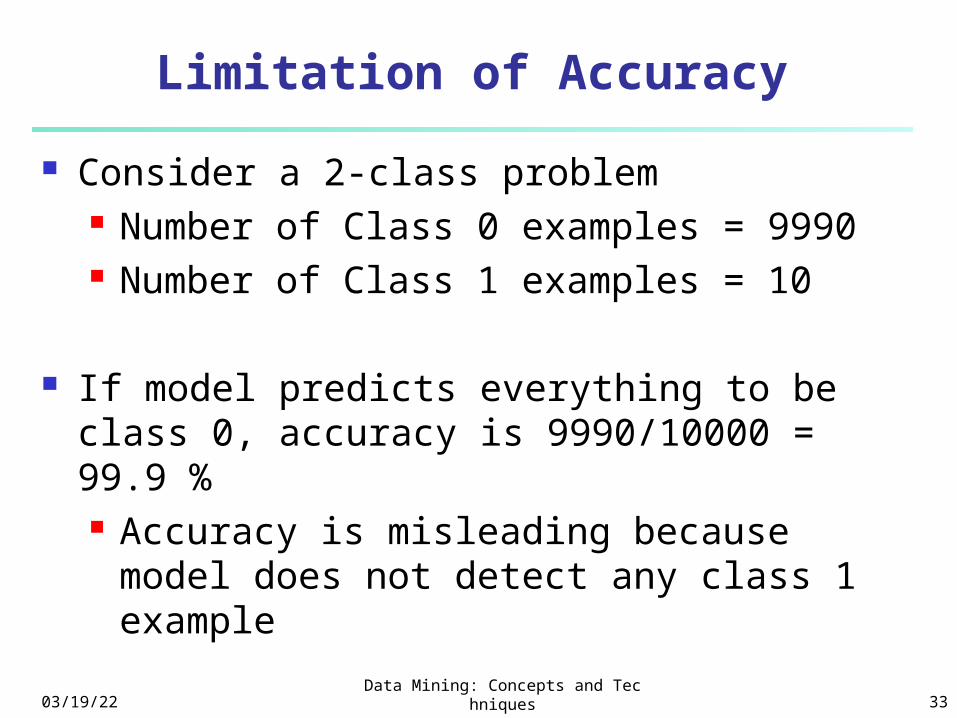
Limitation of Accuracy
Consider a 2-class problem Number of Class 0 examples = 9990 Number of Class 1 examples = 10
If model predicts everything to be class 0, accuracy is 9990/10000 = 99.9 % Accuracy is misleading because model
does not detect any class 1 example
04/19/23Data Mining: Concepts and Technique
s 34
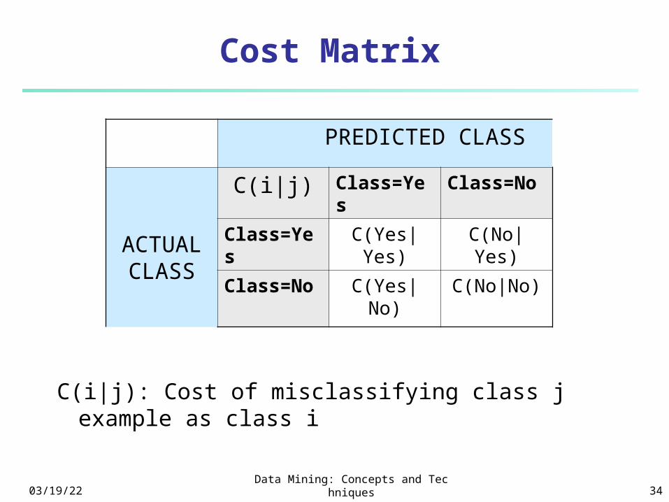
Cost Matrix
PREDICTED CLASS
ACTUALCLASS
C(i|j) Class=Yes
Class=No
Class=Yes
C(Yes|Yes)
C(No|Yes)
Class=No
C(Yes|No) C(No|No)
C(i|j): Cost of misclassifying class j example as class i
04/19/23Data Mining: Concepts and Technique
s 35
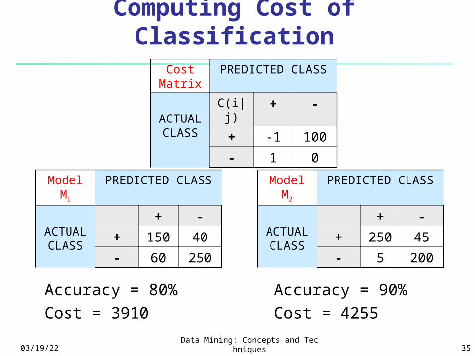
Computing Cost of Classification
Cost Matrix
PREDICTED CLASS
ACTUALCLASS
C(i|j) + -
+ -1 100
- 1 0
Model M1
PREDICTED CLASS
ACTUALCLASS
+ -
+ 150 40
- 60 250
Model M2
PREDICTED CLASS
ACTUALCLASS
+ -
+ 250 45
- 5 200
Accuracy = 80%
Cost = 3910
Accuracy = 90%
Cost = 4255
04/19/23Data Mining: Concepts and Technique
s 36
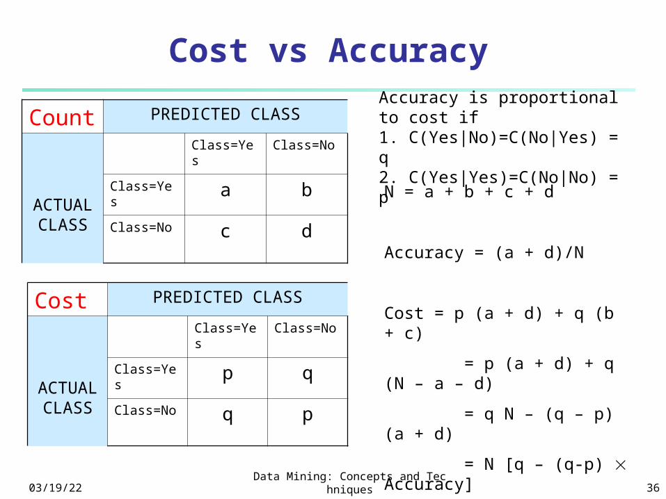
Cost vs Accuracy
Count PREDICTED CLASS
ACTUALCLASS
Class=Yes Class=No
Class=Yes a b
Class=No c d
Cost PREDICTED CLASS
ACTUALCLASS
Class=Yes
Class=No
Class=Yes
p q
Class=No q p
N = a + b + c + d
Accuracy = (a + d)/N
Cost = p (a + d) + q (b + c)
= p (a + d) + q (N – a – d)
= q N – (q – p)(a + d)
= N [q – (q-p) Accuracy]
Accuracy is proportional to cost if1. C(Yes|No)=C(No|Yes) = q 2. C(Yes|Yes)=C(No|No) = p
04/19/23Data Mining: Concepts and Technique
s 37
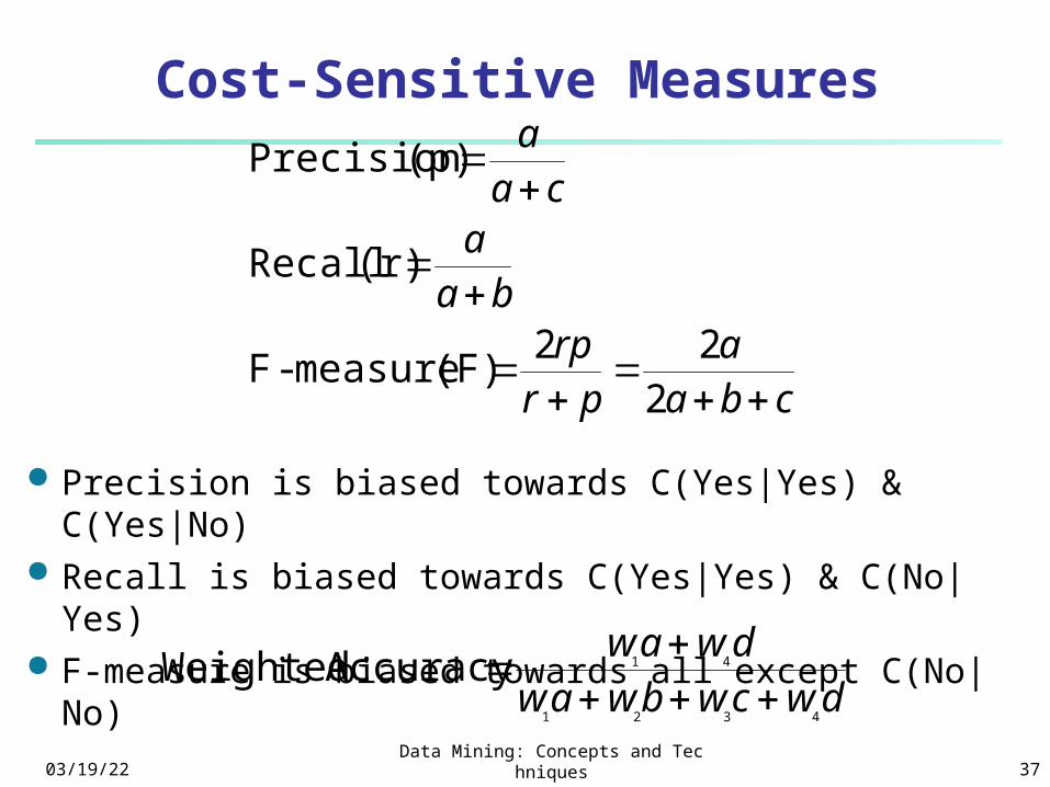
Cost-Sensitive Measures
cbaa
prrp
baa
caa
222
(F) measure-F
(r) Recall
(p)Precision
Precision is biased towards C(Yes|Yes) & C(Yes|No) Recall is biased towards C(Yes|Yes) & C(No|Yes) F-measure is biased towards all except C(No|No)
dwcwbwawdwaw
4321
41Accuracy Weighted
04/19/23Data Mining: Concepts and Technique
s 38
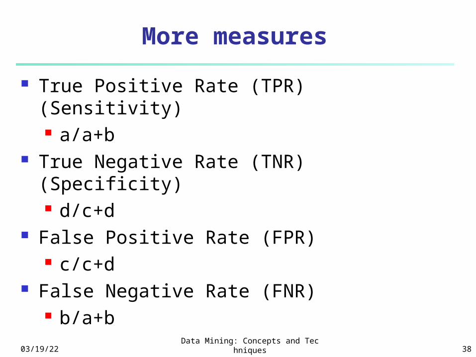
More measures
True Positive Rate (TPR) (Sensitivity) a/a+b
True Negative Rate (TNR) (Specificity) d/c+d
False Positive Rate (FPR) c/c+d
False Negative Rate (FNR) b/a+b
04/19/23Data Mining: Concepts and Technique
s 39
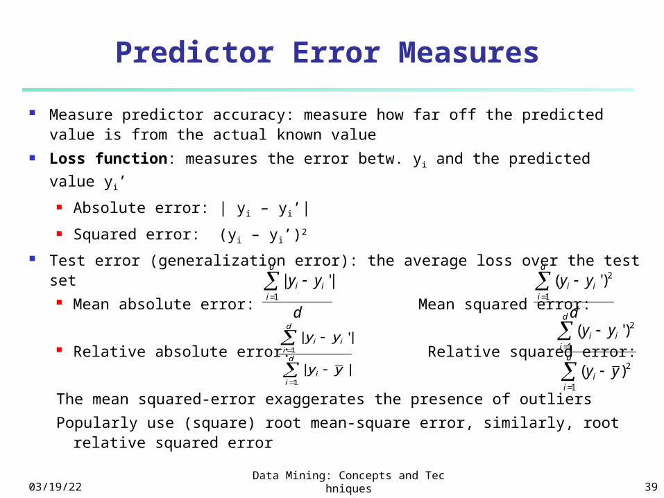
Predictor Error Measures
Measure predictor accuracy: measure how far off the predicted value is from the actual known value
Loss function: measures the error betw. yi and the predicted value
yi’
Absolute error: | yi – yi’|
Squared error: (yi – yi’)2
Test error (generalization error): the average loss over the test set Mean absolute error: Mean squared error:
Relative absolute error: Relative squared error:
The mean squared-error exaggerates the presence of outliers
Popularly use (square) root mean-square error, similarly, root relative squared error
d
yyd
iii
1
|'|
d
yyd
iii
1
2)'(
d
ii
d
iii
yy
yy
1
1
||
|'|
d
ii
d
iii
yy
yy
1
2
1
2
)(
)'(
04/19/23Data Mining: Concepts and Technique
s 40
Chapter 6. Classification and Prediction
What is classification? What
is prediction?
Issues regarding
classification and prediction
Classification by decision
tree induction
Bayesian classification
Rule-based classification
Classification by back
propagation
Support Vector Machines
(SVM)
Associative classification
Lazy learners (or learning
from your neighbors)
Other classification methods
Prediction
Accuracy and error measures
Ensemble methods
Model selection
Summary
04/19/23Data Mining: Concepts and Technique
s 41
Ensemble Methods
Construct a set of classifiers from the training data
Predict class label of previously unseen records by aggregating predictions made by multiple classifiers
04/19/23Data Mining: Concepts and Technique
s 42
Ensemble Methods: Increasing the Accuracy
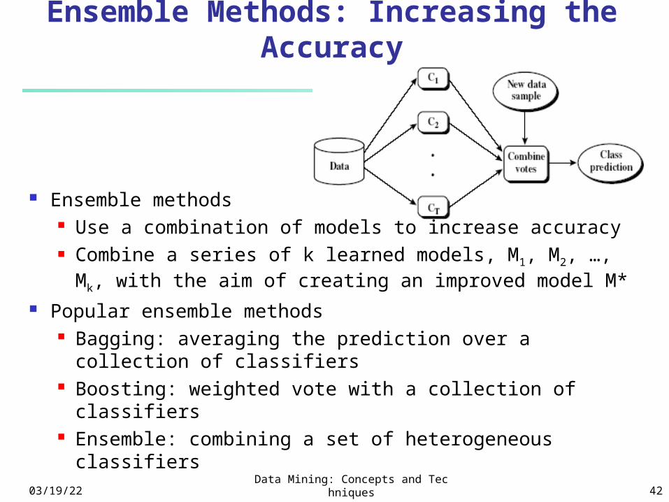
Ensemble methods Use a combination of models to increase accuracy Combine a series of k learned models, M1, M2, …, Mk,
with the aim of creating an improved model M* Popular ensemble methods
Bagging: averaging the prediction over a collection of classifiers
Boosting: weighted vote with a collection of classifiers Ensemble: combining a set of heterogeneous classifiers
04/19/23Data Mining: Concepts and Technique
s 43
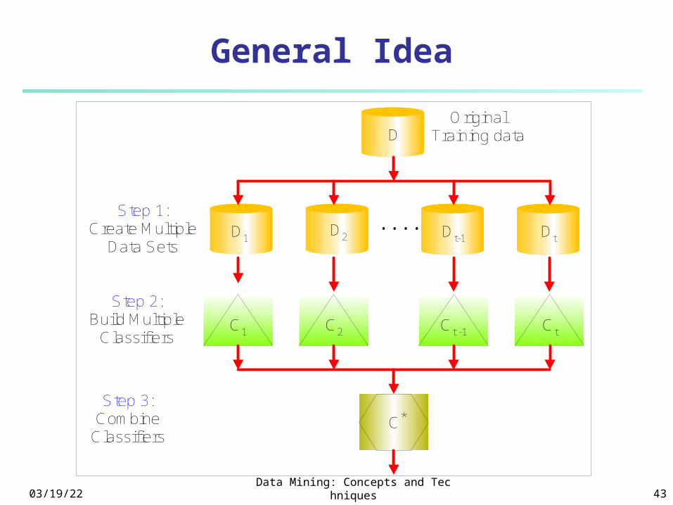
General Idea
OriginalTraining data
....D1D2 Dt-1 Dt
D
Step 1:Create Multiple
Data Sets
C1 C2 Ct -1 Ct
Step 2:Build Multiple
Classifiers
C*Step 3:
CombineClassifiers
04/19/23Data Mining: Concepts and Technique
s 44
Why does it work?
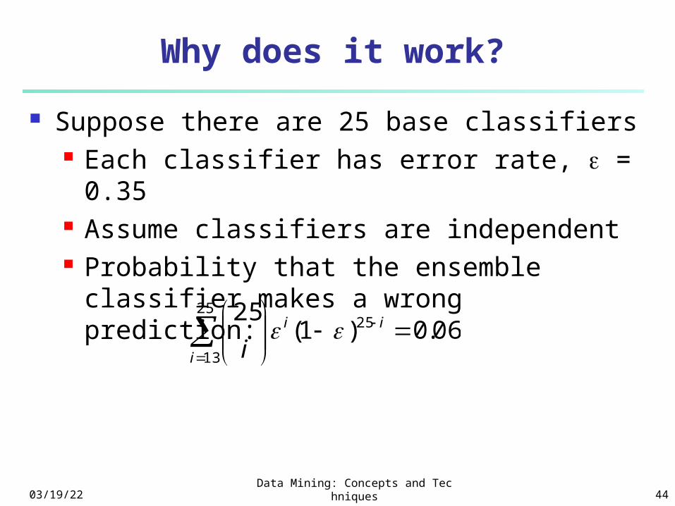
Suppose there are 25 base classifiers Each classifier has error rate, = 0.35 Assume classifiers are independent Probability that the ensemble classifier
makes a wrong prediction:
25
13
25 06.0)1(25
i
ii
i
04/19/23Data Mining: Concepts and Technique
s 45
Examples of Ensemble Methods
How to generate an ensemble of classifiers? Bagging
Boosting
04/19/23Data Mining: Concepts and Technique
s 46
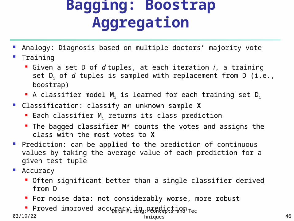
Bagging: Boostrap Aggregation
Analogy: Diagnosis based on multiple doctors’ majority vote Training
Given a set D of d tuples, at each iteration i, a training set Di of d tuples is sampled with replacement from D (i.e., boostrap)
A classifier model Mi is learned for each training set Di
Classification: classify an unknown sample X Each classifier Mi returns its class prediction The bagged classifier M* counts the votes and assigns the
class with the most votes to X Prediction: can be applied to the prediction of continuous values
by taking the average value of each prediction for a given test tuple
Accuracy Often significant better than a single classifier derived from D For noise data: not considerably worse, more robust Proved improved accuracy in prediction
04/19/23Data Mining: Concepts and Technique
s 47
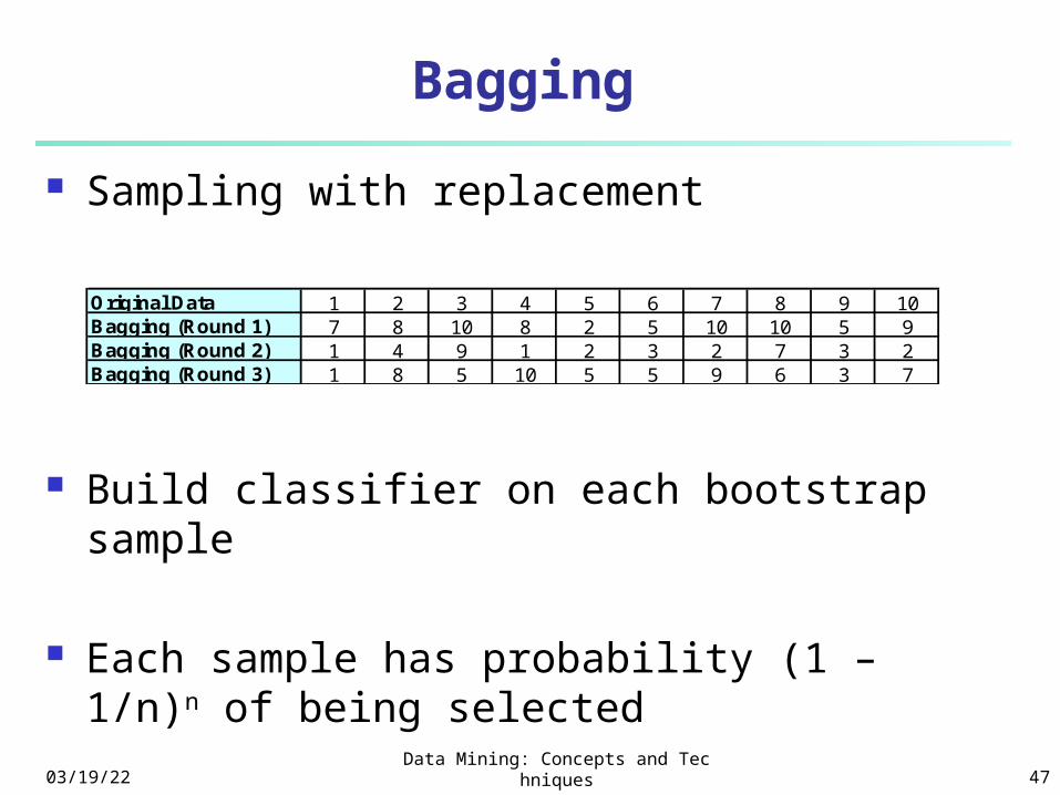
Bagging
Sampling with replacement
Build classifier on each bootstrap sample
Each sample has probability (1 – 1/n)n of being selected
Original Data 1 2 3 4 5 6 7 8 9 10Bagging (Round 1) 7 8 10 8 2 5 10 10 5 9Bagging (Round 2) 1 4 9 1 2 3 2 7 3 2Bagging (Round 3) 1 8 5 10 5 5 9 6 3 7
04/19/23Data Mining: Concepts and Technique
s 48
Boosting
An iterative procedure to adaptively change distribution of training data by focusing more on previously misclassified records Initially, all N records are assigned equal
weights Unlike bagging, weights may change at
the end of boosting round
04/19/23Data Mining: Concepts and Technique
s 49
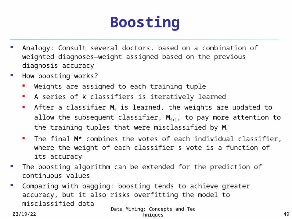
Boosting
Analogy: Consult several doctors, based on a combination of weighted diagnoses—weight assigned based on the previous diagnosis accuracy
How boosting works? Weights are assigned to each training tuple A series of k classifiers is iteratively learned After a classifier Mi is learned, the weights are updated to allow
the subsequent classifier, Mi+1, to pay more attention to the
training tuples that were misclassified by M i
The final M* combines the votes of each individual classifier, where the weight of each classifier's vote is a function of its accuracy
The boosting algorithm can be extended for the prediction of continuous values
Comparing with bagging: boosting tends to achieve greater accuracy, but it also risks overfitting the model to misclassified data
04/19/23Data Mining: Concepts and Technique
s 50
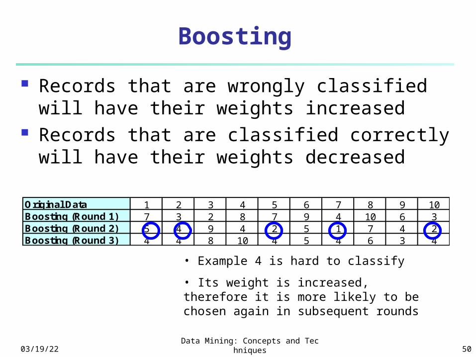
Boosting
Records that are wrongly classified will have their weights increased
Records that are classified correctly will have their weights decreased
Original Data 1 2 3 4 5 6 7 8 9 10Boosting (Round 1) 7 3 2 8 7 9 4 10 6 3Boosting (Round 2) 5 4 9 4 2 5 1 7 4 2Boosting (Round 3) 4 4 8 10 4 5 4 6 3 4
• Example 4 is hard to classify
• Its weight is increased, therefore it is more likely to be chosen again in subsequent rounds
04/19/23Data Mining: Concepts and Technique
s 51
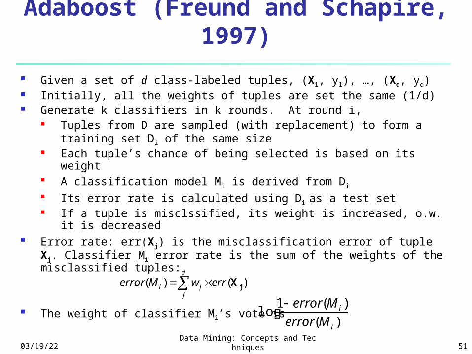
Adaboost (Freund and Schapire, 1997)
Given a set of d class-labeled tuples, (X1, y1), …, (Xd, yd) Initially, all the weights of tuples are set the same (1/d) Generate k classifiers in k rounds. At round i,
Tuples from D are sampled (with replacement) to form a training set Di of the same size
Each tuple’s chance of being selected is based on its weight A classification model Mi is derived from Di
Its error rate is calculated using Di as a test set If a tuple is misclssified, its weight is increased, o.w. it is
decreased Error rate: err(Xj) is the misclassification error of tuple Xj.
Classifier Mi error rate is the sum of the weights of the misclassified tuples:
The weight of classifier Mi’s vote is )(
)(1log
i
i
Merror
Merror d
jji errwMerror )()( jX
04/19/23Data Mining: Concepts and Technique
s 52
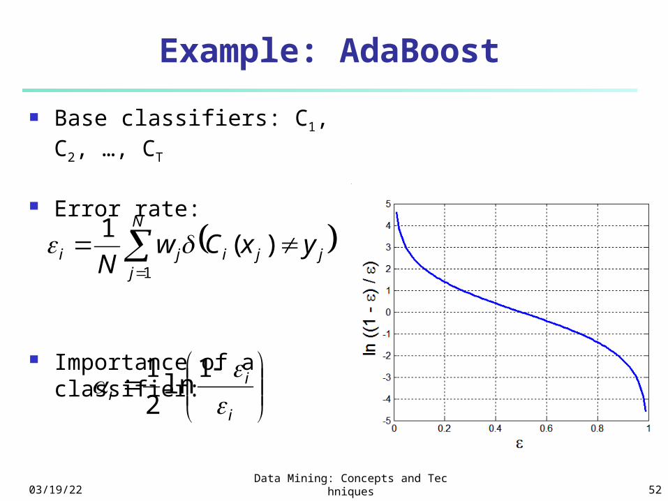
Example: AdaBoost
Base classifiers: C1, C2, …, CT
Error rate:
Importance of a classifier:
N
jjjiji yxCw
N 1
)(1
i
ii
1ln
2
1
04/19/23Data Mining: Concepts and Technique
s 53
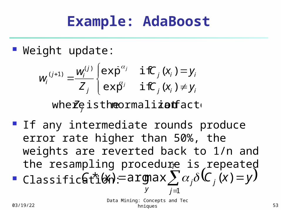
Example: AdaBoost
Weight update:
If any intermediate rounds produce error rate higher than 50%, the weights are reverted back to 1/n and the resampling procedure is repeated
Classification:
factor ionnormalizat theis where
)( ifexp
)( ifexp)()1(
j
iij
iij
j
jij
i
Z
yxC
yxC
Z
ww
j
j
T
jjj
yyxCxC
1
)(maxarg)(*
04/19/23Data Mining: Concepts and Technique
s 54
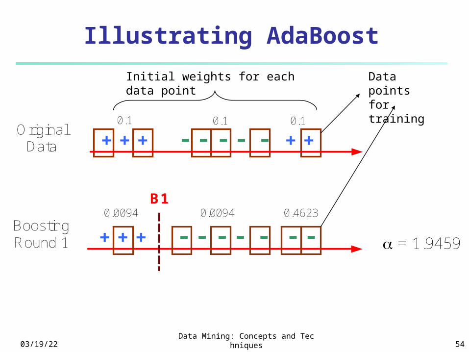
BoostingRound 1 + + + -- - - - - -
0.0094 0.0094 0.4623B1
= 1.9459
Illustrating AdaBoost
Data points for training
Initial weights for each data point
OriginalData + + + -- - - - + +
0.1 0.1 0.1
04/19/23Data Mining: Concepts and Technique
s 55
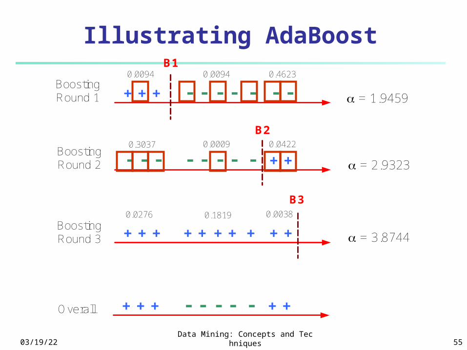
Illustrating AdaBoost
BoostingRound 1 + + + -- - - - - -
BoostingRound 2 - - - -- - - - + +
BoostingRound 3 + + + ++ + + + + +
Overall + + + -- - - - + +
0.0094 0.0094 0.4623
0.3037 0.0009 0.0422
0.0276 0.1819 0.0038
B1
B2
B3
= 1.9459
= 2.9323
= 3.8744