1 SPARQL Language Overview

Scientific SPARQL query language is a superset of the W3C SPARQL 1.1 Standard, and is designed to query RDF with Arrays datasets. The semantics of SciSPARQL is thus focused both on graph pattern matching, defined by the SPARQL standard, and on array processing introduced in our extension

The purpose of this section is to introduce the essential features of SPARQL, as specified by the W3C Standard, including different kinds of graph patterns (basic, optional, alternative), property path expressions, filters, grouping and aggregation. W3C SPARQL 1.1 Specification can also be recommended as a tutorial for the standard language.

The next part continues this overview by discussing the extensions introduced in SciSPARQL, including array expressions, parameterized views, lexical closures, and second-order functions. Together these features make a noticeable shift towards a functional query language, albeit retaining the property of declarativeness.

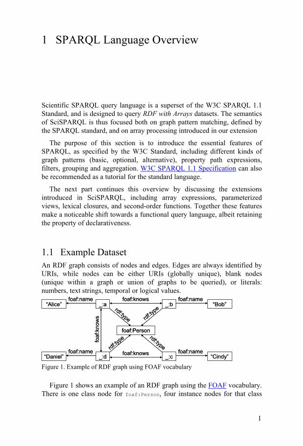
1.1 Example Dataset An RDF graph consists of nodes and edges. Edges are always identified by URIs, while nodes can be either URIs (globally unique), blank nodes (unique within a graph or union of graphs to be queried), or literals: numbers, text strings, temporal or logical values.

“Cindy”foaf:name

_:c

rdf:type

foaf:Person

“Bob”foaf:name

_:b

foaf:knows

“Alice”foaf:name

_:a

“Daniel”foaf:name

_:d

rdf:ty

pe

rdf:ty

perdf:type

foaf:knows

foaf

:kno

ws

“Cindy”foaf:name

_:c

rdf:type

foaf:Person

“Bob”foaf:name

_:b

foaf:knows

“Alice”foaf:name

_:a

“Daniel”foaf:name

_:d

rdf:ty

pe

rdf:ty

perdf:type

foaf:knows

foaf

:kno

ws

Figure 1. Example of RDF graph using FOAF vocabulary

Figure 1 shows an example of an RDF graph using the FOAF vocabulary. There is one class node for foaf:Person, four instance nodes for that class

1

identified by blank nodes, and a foaf:name property for each of them. Additionally they participate in the foaf:knows relationships, which happen to be symmetric - double-sided arrows indicate pairs of symmetric properties.

At the same time, an RDF graph is also a set of (subject, property, value)1 triples. Subject and value of each triple correspond to nodes in the graph, while properties corresponds to edges.

1.1.1 Turtle Syntax There is a number of ways to serialize RDF graphs to text. The RDF graph in Figure 1 can be expressed as a set of triples, e.g.

_:a a foaf:Person ; foaf:name "Alice" ; foaf:knows _:b , _:d . _:b foaf:knows _:a . ...

Throughout this Thesis we will use Turtle - Terse RDF Triple Language to present the RDF datasets. The fully specified triples are separated by dot '.', while triples sharing the same subject are separated by semicolon ';', and triples sharing both subject and property are separated by comma ',', and we usually place them in the same line. So the above fragment contains five triples, with two unique subjects and four unique subject-property pairs. The same syntax is used for specifying triple patterns in SPARQL, as shown in Section 1.2.

Generally, the dot sign separating the triples in RDF and SPARQL has the semantics of a conjunction (along with comma and semicolon). So what technically appears to be a set of triples, from the epistemological perspective is a conjunction of facts.

Both Turtle and SPARQL use prefixes in order to abbreviate URIs. The Turtle file with the dataset on Figure 1 would contain a prefix definition

@prefix foaf: <http://xmlns.com/foaf/0.1/> .

It specifies that e.g. foaf:name property is a shorthand for the URI <http://xmlns.com/foaf/0.1/name>. The reserved property a stands for <http://www.w3.org/1999/02/22-rdf-syntax-ns#type>, otherwise commonly abbreviated as rdf:type. It indicates the relationship between instances and classes when both are represented by RDF nodes.

1 Another common way to refer to triple components is (subject, predicate, object). We prefer to avoid the confusion with ObjectLog predicates.

2

Blank nodes, e.g. _:a are used whenever no URI is provided to identify the node, and different blank node labels specify different nodes. Blank nodes are typically used to represent instances identified by the values of their key properties (as foaf:Person intances are identified by foaf:name values in our example). Another common use case are linked lists, formed with rdf:first and rdf:rest properties. Turtle has a compact syntax to represent such lists, e.g the following Turtle construct:

:s :p ((1 2) (3 4)) .

It encodes a graph, with six blank nodes generated by the Turtle reader, along with 12 triples of the hierarchical linked list.

1.2 Graph Patterns At the core of all non-trivial SPARQL queries there is at least one graph pattern, for example

PREFIX foaf: <http://xmlns.com/foaf/0.1/> SELECT ?person WHERE { ?person foaf:name "Alice" }

contains a graph pattern

?person “Alice”foaf:name

This graph pattern consists of a single triple pattern, with the variable ?person used as a wildcard to match a graph node. The result of such a query would be the set of bindings for the projected variable ?person. If applied to the dataset on Figure 1, this would result in a single blank node _:a.

A graph pattern may be more complex and include a conjunction of several triple patterns, connected with the '.' operator. Whenever the triple patterns have the same subject, '.' is substituted with ';' for a more compact syntax2:

PREFIX foaf: <http://xmlns.com/foaf/0.1/> SELECT ?friend_name WHERE { ?person foaf:name "Alice" ; foaf:knows ?friend . ?friend foaf:name ?friend_name }

2 ... and whenever the triple patterns have the same subject and property, comma sign ',' is used to connect them - similarly to the Turtle syntax explained in Section 1.1.1.

3

Here we need to distinguish between the query results, which contain the binding only for the projected variable ?friend_name, and the solutions, which contain the bindings for all variables in the WHERE block. Given the dataset on Figure 1, the solutions would consist of:

?person ?friend ?friend_name _:a _:b "Bob" _:a _:d "Daniel"

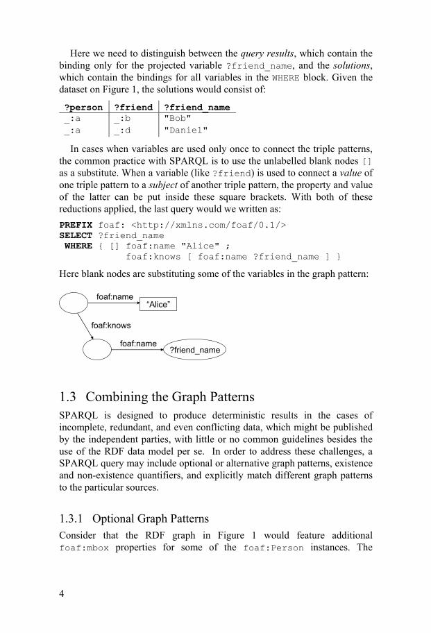
In cases when variables are used only once to connect the triple patterns, the common practice with SPARQL is to use the unlabelled blank nodes [] as a substitute. When a variable (like ?friend) is used to connect a value of one triple pattern to a subject of another triple pattern, the property and value of the latter can be put inside these square brackets. With both of these reductions applied, the last query would we written as:

PREFIX foaf: <http://xmlns.com/foaf/0.1/> SELECT ?friend_name WHERE { [] foaf:name "Alice" ; foaf:knows [ foaf:name ?friend_name ] }

Here blank nodes are substituting some of the variables in the graph pattern:

“Alice”foaf:name

foaf:name?friend_name

foaf:knows

1.3 Combining the Graph Patterns SPARQL is designed to produce deterministic results in the cases of incomplete, redundant, and even conflicting data, which might be published by the independent parties, with little or no common guidelines besides the use of the RDF data model per se. In order to address these challenges, a SPARQL query may include optional or alternative graph patterns, existence and non-existence quantifiers, and explicitly match different graph patterns to the particular sources.

1.3.1 Optional Graph Patterns Consider that the RDF graph in Figure 1 would feature additional foaf:mbox properties for some of the foaf:Person instances. The

4

following query will return the emails of Alice friends, if they are available, and return their names in any case:

PREFIX foaf: <http://xmlns.com/foaf/0.1/> SELECT ?friend_name ?friend_email WHERE { ?person foaf:name "Alice" ; foaf:knows ?friend . ?friend foaf:name ?friend_name . OPTIONAL { ?friend foaf:mbox ?friend_email } }

The nested OPTIONAL graph pattern is thus a source of unbound values in both query solutions and the results of the query:

?friend_name ?friend_email "Bob" mailto:bob@example.org "Daniel"

Being largely similar to the relational algebra left outer join operator applied to the sets of solutions, the OPTIONAL keyword in SPARQL introduces certain issues with declarativeness. In short, there are cases where moving around two OPTIONAL graph patterns may result in a non-equivalent query.

1.3.2 Matching Alternatives Assume some of the emails in the graph are listed using the FOAF standard foaf:mbox property, while others use a domain-specific property <http://example.org/email>. There are two ways to address this inconsistency. The general Semantic Web approach would use an OWL equivalence statement owl:sameAs, so that all SPARQL queries, with OWL entailment enabled, would treat these two properties as equivalent in all RDF graphs.

However, one might instead prefer to treat a set of properties as equivalent just for the purpose of a specific SPARQL query, without manipulating the datasets and affecting the results of other queries. This would be one of the use cases for the alternative graph patterns, combined with UNION, as in the query:

PREFIX foaf: <http://xmlns.com/foaf/0.1/> PREFIX ex: <http://example.org/> SELECT ?friend_name ?friend_email WHERE { ?person foaf:name "Alice" ; foaf:knows ?friend . ?friend foaf:name ?friend_name . { ?friend foaf:mbox ?friend_email } UNION { ?friend ex:email ?friend_email } }

5

Arbitrary graph patterns can be used as alternatives. For the purpose of another example, consider that the foaf:knows relationship is not restricted to be symmetric in the dataset, so we would like to trace it in either direction. The following query returns the names of all people who know Alice and all people whom Alice knows:

PREFIX foaf: <http://xmlns.com/foaf/0.1/> SELECT ?friend_name WHERE { ?friend foaf:name ?friend_name . ?alice foaf:name "Alice" . { ?alice foaf:knows ?friend } UNION { ?friend foaf:knows ?alice } }

This query will effectively express two alternative graph patterns:

?alice “Alice”foaf:name

?friendfoaf:name

?friend_name

foaf:knows

?friend

“Alice”

foaf:name

?alicefoaf:name

?friend_name

foaf:knows

However, if the foaf:knows relationship happens to be mutual in some case, the same bindings will be generated twice for ?friend and ?friend_name. To avoid this, and return every person at most once, one would use DISTINCT option on the ?friend variable in the SELECT clause:

SELECT DISTINCT ?friend ?friend_name

Different branches of the same union might provide bindings for the different variables. For example, the following query might return a more informative result, while generating some unbound values as well:

PREFIX foaf: <http://xmlns.com/foaf/0.1/> SELECT ?name_Alice_knows ?name_knows_Alice WHERE { ?alice foaf:name "Alice" . { ?alice foaf:knows [ foaf:name ?friend_name] } UNION { [] foaf:knows ?alice ; foaf:name ?friendOf_name } }

1.3.3 Existence Quantifiers and Other Filters The presence of at least a single solution to a graph pattern, or the absence of such, can be turned into a Boolean value using the existence quantifiers. For example, the following query checks for the persons who have foaf:homepage property but no foaf:mbox property:

6

PREFIX foaf: <http://xmlns.com/foaf/0.1/> SELECT ?name_Alice_knows ?name_knows_Alice WHERE { ?p rdf:type foaf:Person . FILTER ( EXISTS { ?p foaf:homepage [] } && NOT EXISTS { ?p foaf:mbox [] } ) }

The FILTER conditions in SPARQL queries may appear in a conjunction with graph patterns. They may contain any kind of logical expression, using the logical '&&' (conjunction), '||' (disjunction), and '!' (negation) operators. Besides the quantifiers used in these examples, a large variety of arithmetic and string expressions can be used as terms in the filter conditions. If a filter expression evaluates to anything else than a Boolean value, the Effective Boolean Value of the expression is used. The values equivalent to true are non-zero numbers, non-empty strings and typed RDF literals, all possible date/time values and URIs.

1.3.4 Addressing Multiple Graphs The queries presented so far did not explicitly identify the dataset they address - in this case, they were accessing the default graph of the SPARQL endpoint they are sent to. In the Semantic Web context, a multitude of graphs is typically combined for the purpose of querying. An explicit set of graphs to be combined can thus be specified in the FROM clause of a SPARQL query. Another option is to treat these graphs separately, addressing the specific graph patterns to each of them.

W3C Specifications suggest the following example (presented here with minor simplifications):

PREFIX foaf: <http://xmlns.com/foaf/0.1/> SELECT ?who ?g ?mbox FROM NAMED <http://example.org/alice> FROM NAMED <http://example.org/bob> WHERE { ?who foaf:made ?g GRAPH ?g { ?x foaf:mbox ?mbox } }

This query retrieves the foaf:mbox information from either of the named source graphs, and returns it along with the source graph identifier and the publisher. Here, the graph pattern querying for the foaf:mbox property is matched against every available graph, which is listed in the default graph as a value in a foaf:made triple.

1.4 Property Path Expressions A powerful feature introduced in the W3C SPARQL 1.1 Standard are regular path expressions as another kind of graph patterns, making it easy to

7

specify chains of properties, alternative and reversed properties. For example, the first two queries in Section 1.3.2 can be reformulated using patterns like

?friend foaf:mbox|ex:email ?friend_email

and

?alice foaf:knows|^foaf:knows ?friend

respectively, where the '|' operator denotes the alternatives and '^' specifies the reversed property.

Still, the main power of the regular path expressions is the ability to query for graph nodes connected by chains of properties of arbitrary length but with certain repeating structure. For example, the following query would list the names of people who are listed as Alice's friend, friend-of-a-friend (that's what FOAF vocabulary name actually stands for), and so on:

PREFIX foaf: <http://xmlns.com/foaf/0.1/> SELECT ?friend_name WHERE { [] foaf:name "Alice" ; foaf:knows+/foaf:name ?friend_name }

Here the '+' operator denotes the transitive closure of the foaf:knows property, and '/' denotes the chaining of property paths. If the '*' operator were used instead of '+', the reflexive-transitive closure would include "Alice" among the results.

The transitive and reflexive-transitive closures are implemented as graph traversal algorithms, which internally check for equivalence of the nodes, and terminate at the point where no new nodes can be reached.

1.4.1 Precedence of Path Operators Path operators can be freely combined in a path expression. According to W3C SPARQL 1.1 Specifications the precedence order of the path operators3 is the following:

transitive '+', reflexive '?', and reflexive-transitive closure '*' reversal '^' chaining '/' alternative paths '|'

3 We do not include the negated property set operator in the current version of SciSPARQL, due to the problems with its standard definition, explored in [88]. Though not theoretically ambiguous, together with reversal it introduces certain counter-intuitive 'butterfly effect' in the set of query solutions.

8

Whenever a different precedence is desired, parentheses can be used to control associatively. For example, a graph pattern

?x (ex:motherOf|ex:fatherOf)+/foaf:name "Alice"

would bind ?x to all ancestors of a person named Alice.

1.4.2 Algebraic Properties of Path Operators Even though the W3C Standard does not list the properties of path operators explicitly, they are trivial to deduce, and are invaluable if one would like to transform the regular path expressions within their class of equivalence, for the purpose of simplification or normalization. The SPARQL users, formulating queries with path expressions, might also benefit from the structured summary presented in this section.

In the following triangular table (Table 1) we summarize the equivalent expressions that arise when one or two path operators are combined. Given A, B, and C are path fragments, the identities listed in the table cells always hold.

Table 1. Algebraic properties of path operators + * ? ^ / |

+ A++ = A+ (A+)* = A*(A*)+ = A*

(A?)+ = A* ^A+ = (^A)+ - -

* A** = A* (A?)* = A*(A*)? = A*

^A* = (^A)* - -

? A?? = A? ^A? = (^A)* - - ^ ^^A = A ^(A/B) = ^B/^A ^(A|B) = ^A|^B

/ A/(B/C) = = (A/B)/C

(A|B)/C = A/C|B/C A/(B|C) = A/B|A/C

| A|B = B|A

A|(B|C) = (A|B)|C

In mathematical terms, Table 1 lists the following properties: idempotence of closure operators '+', '*', and '?', subsumption of transitive '+' and reflexive '?' closures into the

reflexive-transitive closure '*' - the latter can also be constructed by applying transitive closure '+' on top of the reflexive closure '?' (but not the other way around),

involution property of the reversal operator '^', commutative property of the alternative operator '|', self-distributiveness and mutual distributiveness of chaining '/' and

alternative '|' operators, distributiveness of the reversal operator '^' with respect to closures

and the alternative '|' operator, and reversal of the chains of path fragments with the reversal operator '^'.

9

1.5 Aggregation and Grouping The SELECT part of a SPARQL query may contain a list of projected variables (as seen in all the queries presented so far), or named expressions. A variety of functions, including arithmetic and string manipulation, are available, and, in the case of SciSPARQL, easily extensible, as we show in Section 2.4. For example a query with the SELECT statement

SELECT (round(?x) AS ?result) ...

would return the rounded value for each ?x binding among the query solutions, i.e. the round() function will be applied independently every time the query is about to emit.

There are, however, certain SPARQL functions which operate on bags (multisets) of bindings - the aggregate functions. Most of them, like SUM(), AVG() etc. operate only on numerical values, whereas COUNT() operates on all kinds of values. For example, the following query would return minimum and maximum age of persons listed in the graph:

PREFIX foaf: <http://xmlns.com/foaf/0.1/> SELECT (MIN(?age) AS ?min_age) (MAX(?age) AS ?max_age) WHERE { ?p rdf:type foaf:Person ; foaf:age ?age }

emitting a single result (or none if no persons or their age information is found).

If one would need to compute e.g. the average age of each persons friends, this would require grouping the query solutions by person, and applying the aggregate AVG() function within each group. This is achieved with the GROUP BY clause:

PREFIX foaf: <http://xmlns.com/foaf/0.1/> SELECT ?name (AVG(?friend_age) AS ?avg_friend_age) WHERE { ?p rdf:type foaf:Person ; foaf:name ?name ; foaf:knows ?friend . ?friend foaf:age ?friend_age } GROUP BY ?p ?name

Note that we need to group by the variable ?p, bound to foaf:Person instance nodes, not by the person name (which might not be unique). Listing ?name as an additional grouping variable might seem redundant, as ?name is fully functionally dependent on ?p, i.e. we do not expect different ?name values for the same person. Unfortunately, SPARQL requires that every variable projected out from the aggregate query (or used for post-filtering or ordering) should be also listed in GROUP BY clause. In SciSPARQL we lift this restriction, implicitly adding such variables to the effective GROUP BY clause.

10

Additional post-filter conditions can make use of the aggregate values computed. For example, adding

HAVING (?avg_friend_age <= 30 && COUNT(?friend) > 3)

to the end of the last query would restrict the resulting groups of solutions by size and average age. Note that this adds another aggregate value to be computed for each group.

1.6 Error Handling It is worth noting that in SPARQL every valid query is always evaluated without raising any exceptions. This is achieved by two separate mechanisms:

I. The validity of the query can be determined at compile time - a process separate from actually executing the query on a given dataset. A SPARQL query processor emits a wide range of error conditions at different phases of validating the query. The lexical and syntactic errors, corresponding e.g. to an unmatched quotation mark or an unexpected keyword, indicate that the query cannot be reconstructed from a given textual representation. Next, a range of semantic checks is performed - a semantic error can be raised e.g. if aggregate function calls are nested. Finally, the query is transformed to an execution plan, making sure that every variable gets a finite multiset of potential bindings. If this is found impossible, the query will be reported as non-executable.

II. A valid query may still produce errors, when applied to a certain dataset. Division by zero, or a non-numeric operand passed to an arithmetic operator (since SPARQL is dynamically typed) produce a special error value, which is passed further through the expressions. Query solutions containing an error value for a variable never produce a result. Hence, evaluating a FILTER expression to error is equivalent to evaluating it to false. A SELECT expression evaluating to error effectively discards the solution. This includes aggregate functions evaluating once per group.

For example, if a group of solutions contains a non-numeric binding for a variable under SUM(), the aggregate function would return error, and the group will not be part of query result. In our system, returning error value from a function is in all ways equivalent to returning no values at all. Saying that a function does not return in a certain case should be understood as returning error value in the standard SPARQL terms.

11

1.7 Ordering and Segmentation By default, the result of a SPARQL query is a multiset of bindings for the query output variables. It is, however, possible to return these bindings in a certain order, by using the ORDER BY clause.

The following query would list the persons in the dataset sorted by age (in descending order) and, in the case of coevals, by name (alphabetically):

PREFIX foaf: <http://xmlns.com/foaf/0.1/> SELECT ?name ?age WHERE { ?p rdf:type foaf:Person ; foaf:name ?name foaf:age ?age } ORDER BY DESC(?age) ?name

Once the order of the results is defined, it becomes possible to retrieve certain portions of results. For example, adding

LIMIT 3

to the end of the query would make it return the information about the three oldest people (thus probably saving considerably on communication), and adding instead

OFFSET 500 LIMIT 100

would be typical for a query retrieving the portions of results on demand.

Since the SPARQL standard specifies that the comparison '<' and '>' operators are defined only on the values of the same type, the order of results where an ordering variable is bound to values of the different (incomparable) types is not defined, and hence the segmentation cannot be used in the reliable way. SciSPARQL addresses this problem by defining a certain order among the values of all possible types in RDF with Arrays, including URIs, blank nodes, all kinds of literals and arrays.

1.8 Constructing New RDF Graphs As mentioned before, the result of a SELECT query in SPARQL is a list of mappings of its output variables to values (which might include unbound values). Sometimes, it is instead desirable to produce a set of triples, which can be regarded as a derived RDF graph. For this purpose, CONSTRUCT queries are available in the language4.

4 The W3C SPARQL standard also specifies ASK queries, wich are the shorthand of using EXISTS quantifier, and mentions DESCRIBE queries, not actually defined in the standard.

12

The following query would construct a derived graph, listing ex:mutualFriend properties for all pairs of persons connected with foaf:knows relationship both ways:

PREFIX foaf: <http://xmlns.com/foaf/0.1/> PREFIX ex: <http://example.org/> CONSTRUCT { ?x ex:mutualFriend ?y } WHERE { ?x rdf:type foaf:Person ; foaf:knows ?y ; ?y rdf:type foaf:Person ; foaf:knows ?x }

The CONSTRUCT clause contains a graph construction pattern. For every solution of the WHERE block, the corresponding triples will be constructed and emitted. Note that since the graph pattern in the WHERE clause is symmetric there will be two solutions for each matching pair of persons.

The solutions with unbound variables will not produce triples in those construction patterns where these variables are used.

1.9 Updating the Datasets The separate W3C Standard Recommendation governs the SPARQL Update language.

The Data Definition Language is limited to creating (with the CREATE statement) and dropping (with the DROP statement) the named RDF graphs, since, in contrast to the relational data model, there are no schemas to be defined separately from the data.

The Data Manipulation Language is mainly represented by the DELETE/INSERT statement. For example, instead of deriving a new RDF graph (as in Section 1.8), one could insert the new triples into the same graph, by simply changing the CONSTUCT keyword to INSERT.

Deleting triples is as simple - the following statement would delete all personal emails from the graph:

PREFIX ex: <http://example.org/> DELETE { ?p foaf:mbox ?email } WHERE { ?p rdf:type foaf:Person ; foaf:mbox ?email ;

For every solution of the WHERE block (i.e. for every combination of ?p and corresponding ?email values), this statement will delete all triples according to the deletion triple pattern. In principle, this would be possible to do with some of the pattern variables free, but SPARQL (and the current implementation of SciSPARQL) requires that all delete pattern variables

13

should be bound. It is part of the future work on SciSPARQL to lift this unnecessary restriction.

The DELETE and INSERT clauses can be combined in a single statement, sharing the WHERE block (e.g. for replacing certain properties according to a pattern). Deletion and insertion patterns may include a named GRAPH specifier, similarly to the syntax shown in Section 1.3.4, or a named graph addressed by the whole statement can be specified using the WITH keyword. A different graph can be used in the WHERE block, introduced with the USING keyword instead.

A different mechanism is used for evaluating simple INSERT DATA and DELETE DATA statements: they do not contain a WHERE block, hence their patterns are free from variables and are purely constant. Their purpose is the massive insertion or deletion of RDF triples in a streamed fashion. They are evaluated at parse time, and thus can be arbitrarily long.

14

2 Scientific SPARQL

The main purpose of Scientific SPARQL is to enable data processing tasks common in science and engineering to be expressed as queries in extended SPARQL. These tasks are generally characterized by extensive computations, and also by large amounts of numeric data, typically ordered along a number of orthogonal axes. Such data can be represented as numeric multidimensional arrays, which become a class of RDF terms in our extended RDF with Arrays data model.

Computations are used either for filtering or post-processing the retrieved data, and may typically be expressed in a functional way. Existing computational libraries (many of which became de-facto standards in scientific computing, and are often referred for reproducibility of results) can be interfaced and invoked from the query language as foreign functions. Cost estimates and alternative directions of evaluation can be additionally specified (see Section 2.4), in order to aid the construction of better execution plans.

Though real-life scientific computing tasks find much more compact formulations in SciSPARQL than in high-level algorithmic languages like Matlab (mainly thanks to declarativeness and more natural metadata management), we expect complex tasks to be formulated as complex queries. Good query modularity becomes as important for scalability as good data design and annotation. In this respect, SciSPARQL allows expressing common query sub-tasks as functional views, i.e. SciSPARQL functions defined as parameterized queries.

Such flexibility in defining functions and using them in queries is further strengthened by functional language abstractions such as lexical closures and second-order functions. When it comes to the array processing tasks, besides a library of the most common functions, SciSPARQL offers array constructors, mappers and condensers as second-order functions.

This chapter summarizes the contributions presented in Scientific SPARQL as a language extension in terms of syntax and semantics. Implementation details are reserved for the next chapter, however, certain notes on potential scalability opportunities are given, in order to encourage

15

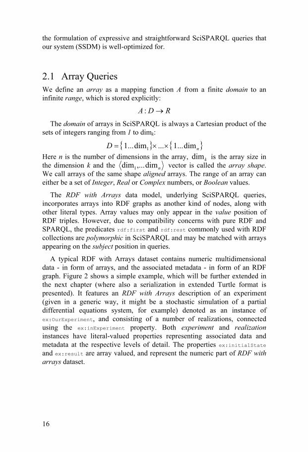
the formulation of expressive and straightforward SciSPARQL queries that our system (SSDM) is well-optimized for.

2.1 Array Queries We define an array as a mapping function A from a finite domain to an infinite range, which is stored explicitly:

RDA :

The domain of arrays in SciSPARQL is always a Cartesian product of the sets of integers ranging from 1 to dimk:

nD dim...1...dim...1 1 Here n is the number of dimensions in the array, kdim is the array size in the dimension k and the ndim,...dim1 vector is called the array shape. We call arrays of the same shape aligned arrays. The range of an array can either be a set of Integer, Real or Complex numbers, or Boolean values.

The RDF with Arrays data model, underlying SciSPARQL queries, incorporates arrays into RDF graphs as another kind of nodes, along with other literal types. Array values may only appear in the value position of RDF triples. However, due to compatibility concerns with pure RDF and SPARQL, the predicates rdf:first and rdf:rest commonly used with RDF collections are polymorphic in SciSPARQL and may be matched with arrays appearing on the subject position in queries.

A typical RDF with Arrays dataset contains numeric multidimensional data - in form of arrays, and the associated metadata - in form of an RDF graph. Figure 2 shows a simple example, which will be further extended in the next chapter (where also a serialization in extended Turtle format is presented). It features an RDF with Arrays description of an experiment (given in a generic way, it might be a stochastic simulation of a partial differential equations system, for example) denoted as an instance of ex:OurExperiment, and consisting of a number of realizations, connected using the ex:inExperiment property. Both experiment and realization instances have literal-valued properties representing associated data and metadata at the respective levels of detail. The properties ex:initialState and ex:result are array valued, and represent the numeric part of RDF with arrays dataset.

16

ex:OurExperiment

ex:OurExperimentRealization

ex:experiment1

_:r1

rdf:type

rdf:type

ex:inExperiment

ex:OurSimulationAlgorithm

ex:simulationMethod

1 ex:id

0.3ex:parameter_A

0.85ex:parameter_B

ex:in

itialS

tate ex:result

ex:OurExperiment

ex:OurExperimentRealization

ex:experiment1

_:r1

rdf:type

rdf:type

ex:inExperiment

ex:OurSimulationAlgorithm

ex:simulationMethod

1 ex:id

0.3ex:parameter_A

0.85ex:parameter_B

ex:in

itialS

tate ex:result

Figure 2. An example RDF with Arrays dataset (fragment)

We will refer to the queries aimed at retrieving arrays from RDF with Arrays datasets, and containing array-specific operations as array queries.

A trivial (but important) case is retrieving an array based on the associated metadata. For example, one might be interested in the ex:result arrays together with the corresponding realization ids, based on the experiment properties and realization parameters:

SELECT ?id, ?A WHERE { ?e a ex:OurExperiment ex:simulationMethod ex:OurSimulationAlgorithm . ?r ex:inExperiment ?e ; ex:parameter_A 0.3 ; ex:parameter_B ?b ; ex:id ?id ; ex:result ?A . FILTER ( ?b > 0.8 ) }

The rest of this section introduces the key features of array queries. In the examples we deliberately omit the PREFIX part of the queries, since SciSPARQL allows the prefix declarations to be specified once per session - with a separate statement:

PREFIX ex: <http://udbl.uu.se/ex#>

2.1.1 Array Dereference Syntax SciSPARQL allows array subscripts in square brackets, where subscripts for the respective dimensions are separated with commas.

For each dimension either single subscripts or range selections can be specified. By default, range selections are specified with a colon as lo:hi,

17

and selections with a stride as lo:stride:hi, where both lo and hi address the elements that are included in the selection, and the elements are counted from 1. This design was chosen to make Matlab users feel at home5.

Either or both lo and hi values can be omitted, with default for lo being 1 and default for hi always being the array size in the respective dimension. Thus the expressions ?A[:] and ?A[:1:] are always equivalent to ?a.

If valid single subscripts for all array dimensions are specified, the array is dereferenced to a single element. Otherwise, complete ranges are assumed for the remaining dimensions. SciSPARQL thus makes a difference between three kinds of array dereferences:

single element dereference, for example ?A[2,1] for a 2D array ?a, where single subscripts are provided for all dimensions. The result is always a number, or error if a subscript falls out of range.

projection dereference, for example ?A[:,1] or ?A[2] or ?A[1:3,2] or ?A[2,:5:] for a 2D array ?A, where single subscripts are provided for some dimensions, and range selections (explicit or implicit) for the others. The result is a smaller array with fewer number of dimensions (only those of the original dimensions for which ranges were provided), or error if a single subscript falls out of range or the range selection results in an empty selection.

range selection dereference, for example ?A[1:5,2:3], ?A[1:5], ?A[:5,:2:], where range selections (explicit or implicit) are provided for all array dimensions. The result is a smaller array with the same number of dimensions as the original one, or error if the range selection results in an empty selection.

The latter two are also collectively called array slicing operations. Each array slicing is resulting in an array subset Figure 3 shows the elements selected from a 2D array using projection on the first (rows) dimension, and range selection on the second (columns) dimension.

5 However, with the _sq_python_ranges_ flag a user may opt for a different dialect of SciSCPARQL, which supports Python notation for ranges. In this case, elements are counted from 0, hi element is never part of the selection, and optional strides are specified as lo:hi:stride. No other differences are introduced. This switch only takes effect at the stage when a SciSPARQL query, update, or function definition is passed to the interpreter. The definitions of SciSPARQL functions and parameterized updates are stored internally in a way that is invariant to these syntactic differences, so it is safe to switch back and forth between the two dialects in a session. In the rest of this work, the default (Matlab) notation is used.

18

pro

ject

ion

i

lo histride

range selection Figure 3. A projection and range selection ?A[4,3:2:7], applied to a 2D array

If a range selection effectively specifies a single element, it is still treated as a range selection with respect to the dimensionality reduction. Thus, (unlike Matlab) SciSPARQL makes a difference between arrays that have different number of "single-element" trailing dimensions, and between singleton arrays and numbers, so that ?A[2,3:3] is not equal to ?A[2,3]. For a 2D array ?A where these subscripts are valid, the former expression would return a 1D-projection with a single element in it, whereas the latter expression would dereference directly to that element.

Since SciSPARQL is designed to handle very large arrays, any dereference operation that returns a derived array does not allocate any memory to store the new array's elements - internally, it just allocates a new descriptor object pointing to the same storage space. Thus, creating sets of projections and slices of arrays is very cheap, and is encouraged as a simple way to formulate many data-reduction operations. This principle extends to arrays stored externally (and retrieved lazily).

2.1.2 Variables Bound to Array Subscripts One important feature of SciSPARQL as a declarative query language is the possibility to automatically bind a query variable to its valid range of values. Just as a triple pattern

?x foaf:name "Alice" .

binds variable ?x to every node that has a property foaf:name with value "Alice", an array dereference expression

?A[?i]

with the otherwise unbound variable ?i becomes an array access pattern: the variable ?i will assume all valid subscript values, that is, integers from 1 and up to the size of array ?A in its first dimension.

Unless otherwise restricted, such binding will form a Cartesian product with bindings for other variables in the query solution. So, for example,

SELECT ?i, ?j (?A[?i,?j] AS ?value) WHERE { [] ex:id 1 ; ex:result ?A }

19

will return every element of the 2D array ?A (or respective projections if ?A is array of grater dimensionality, or nothing otherwise), together with subscript values. Similarly,

SELECT ?i, ?j (?A[?i,?j] AS ?value) WHERE { [] ex:id 1 ; ex:result ?A . FILTER ( ?i >= ?j ) }

will return bottom-left triangle of ?A, and

SELECT ?i (?A[?i,?i] AS ?value) WHERE { [] ex:id 1 ; ex:result ?A }

will return the diagonal elements.

2.1.3 Built-in Array Functions A number of basic functions are defined in SciSPARQL in order to access the array shape and element type, construct arrays and perform operations not covered by the array dereference syntax:

adims(?a) - return the shape of an array as a 1D integer array containing sizes of a in each dimension. To obtain the number of dimensions, use adims(adims(?a))[1].

elttype(?a) - return element type of array, with 0 for Integer, 1 for Double, 2 for Complex.

A(?e1, ?e2, ?e3, ...) - construct a 1D array of the given numeric elements.

find(?a, ?e) - return the indexes of elemets in ?a equal to ?e, as 1D integer arrays.

permute(?a, ?d1, ?d2, ...) - change the shape of array by rearranging its dimensions (generalized transposition). The integer values ?d1, ?d2, ... denote the new order for the array dimensions. The effect the is same as with Matlab permute() function6.

transpose(?a) - simple 2D matrix transposition, equivalent to permute(?a, 2, 1).

Rearranging array dimensions, similarly to an array slicing operation, involves no copying of array elements, and thus produces a derived array.

2.1.4 Array Arithmetic The standard binary operators operating on numbers in SPARQL are extended to operate element-wise on arrays in SciSPARQL. This includes addition '+', subtraction '-', multiplication '*', and division '/' operators. For

6 http://mathworks.com/help/matlab/ref/permute.html

20

example, an expression ?a + ?b will be evaluated in four cases, as shown in the Table 2.

Table 2. Polymorphism of an arithmetic operator in SciSPARQL (example)

?a binding ?b binding value of ?a + ?b number number number number array array, where ?a is added to each element of ?b array number array, where ?b is added to each element of ?a array array array of sums of corresponding ?a and ?b

elements, if ?a and ?b have the same shape

However, in order to let the SciSPARQL query optimizer distinguish between scalar and array-valued operations (the latter are expected to be sufficiently more expensive, both in terms of computation and memory), SciSPARQL users are encouraged to use the special array-oriented dot-prefixed operators, for example '.+' in cases where array values are expected.

The expression ?a .+ ?b is semantically equivalent to ?a + ?b as described by Table 2, e.g. it produces a number if both operands are numbers. However, it hints the query optimizer that an array value is expected here, so it will try to schedule this operation at the point where fewer intermediate results (i.e. candidate bindings for ?a and ?b) are anticipated.

This is different for the comparison operators '<', '<=', '>', '>=', which, when applied to an array (or two arrays of the same shape) will produce a deterministic albeit not a meaningful result, used only for ordering. Equality of arrays, however, is well defined below in Section 2.1.6. In the same cases, dot-prefixed comparison operators will produce a new array of type Boolean, containing the results of element-wise comparison.

Numeric aggregate functions, like SUM(), MIN(), MAX(), AVG(), etc. are also extended to handle bags of array values. They return only if all arrays in the bag have the same shape, and construct a new array value. No optimizer hints are available.

Another possibility is that due to the modular structure of SciSPARQL queries, there might be two parameterized aggregate subqueries invoked as functions from a third query on the same level - then the optimization might benefit from knowing which aggregation involves arrays and which one does not. We leave these optimization opportunities, based on a more accurate cost estimate for the aggregate functions as a matter of the future work.

21

2.1.5 Intra-array Computations Arrays, apart from bags, form another conceptual layer of collections in SciSPARQL. While it is possible to combine all elements of a bag of numbers (or arrays) with the aggregate function SUM(), it should also be possible to apply an aggregate function to all (or certain) elements of a given array. There are actually three ways to do this in SciSPARQL:

I. Shorthand functions as array_sum(), array_avg(), array_min(), and array_max() are available in SciSPARQL for the basic computation tasks, and should be preferred as the most efficient ones. They operate on all elements of a given array, and ignore the logical dimensionality.

II. It is always possible to "open" an array into a bag of its elements, as shown in Section 2.1.2, and then apply a traditional aggregate function. This allows arbitrary conditions on the element places and values to be expressed in a query. For example, the following query would sum up only positive elements on even positions in the main diagonal of ?A:

SELECT (SUM(?A[?i,?i]) AS ?sum_diag_even_positive) WHERE { [] ex:id 1 ; ex:result ?A . FILTER ( ?A[?i,?i] > 0 ) && mod(?i, 2) = 0 }

Here, the free variable ?i binds to all valid values for the row and column subscripts of ?A, and then is checked for an even value. Only in those cases, array elements are considered eligible to be summed up. As the example shows, this way is highly general, but might clutter the FILTER expression (which is typically used for metadata conditions) and also forces bag-based aggregation where it could have been avoided.

III. In order to alleviate for the said shortcomings, SciSPARQL borrows Array Algebra primitives used in Rasdaman, as a matter of ongoing integration. The second-order functions MAP(), CONDENSE(), and ARRAY()are supported in our system, making use of the powerful lexical closure mechanism, explained in Section 2.3.

2.1.6 Array Equality The only cases where dot-prefixed operators differ from the original ones is the comparison of arrays with '=' and '!=', which results in a single Boolean value, and the comparison of array elements with '.=' and '.!=', which results in array of Boolean. While the second case is trivial, the equality of arrays needs a definition.

Two arrays are equal iff all of the following conditions are satisfied: they have the same number of dimensions, they have the same size in each respective dimension, their respective elements are numerically equal.

22

Note that the same element type is not a requirement - an integer array might be equal to an array of real numbers. However, whenever the floating-point arithmetic is involved, it is always a good idea to round the array elements down to a certain precision before comparing, in order to avoid precision-induced artifacts. For this purpose the round() function is extended to handle arrays, taking the desired precision as a second argument.

SciSPARQL does not trim the trailing dimensions of size 1 as e.g. Matlab does, which might lead to the loss of structural metadata, important in our setting. Hence e.g. a 1-dimensional array of size 3 can never be equal to a 2-dimensional 3x1 array, even though they both might represent the same mathematical object - a column vector. Similarly, SciSPARQL does not treat simple numeric values as equivalent to singleton arrays: a number 5 is not equal to an array with a single element of 5.

2.2 Parameterized Queries - Functional Views The good modularity of potentially complex SciSPARQL queries is achieved by isolating common parts as parameterized queries, also known as functional views. We use these two terms interchangeably, since by stressing different aspects of the same mechanism, together they convey the desired dualistic notion of the subject.

There is DEFINE FUNCTION statement in SciSPARQL. As shown below in Section 2.4, its use extends far beyond the functional views and SciSPARQL per se; however, for the purpose of this section its use is quite simple. The following example defines a function resultById() retrieving the value of ex:result property of a realization of the ex:OurExperiment experiment class, given the realization id:

DEFINE FUNCTION resultById(?id) AS SELECT ?A WHERE { ?r ex:inExperiment [ a ex:OurExperiment ] ; ex:id ?id ; ex:result ?A }

Naturally, a call to this function can be used as a part of an expression. This has the potential of formulating short queries without a proper WHERE clause at all. For example, the following query returns the third row of the ex:result matrix of a realization with id = 1:

SELECT (resultById(1)[3] AS ?row3)

A function definition is parsed and validated (but not optimized) at the moment it is submitted as a SciSPARQL statement. This implies, in particular, that the prefixes used in a function definition (unless supplied directly before the DEFINE FUNCTION clause) should be already defined for

23

a session. Similarly, any other functions called inside the definition should already be defined. This way SciSPARQL forbids mutual- and self-recursion, and imposes an acyclic dependency graph among the function definitions it maintains.

This principle does not extend to accessing the named RDF graphs. A graph specified in a FROM, FROM NAMED, or GRAPH clause inside a function definition does not need to be present among the available graphs at the time of function definition - thus the library of functional views can be loaded into a SciSPARQL session (using SOURCE directive) independently of loading or creating the named RDF graphs.

Apart from query modularity benefits, with functional views it is possible to express some otherwise inexpressible computations in a single query. In particular, it is possible to nest aggregate operations - for example computing the sum of positive diagonal elements of ex:result for each array, and then finding the average value across all realizations in the given experiment instance:

DEFINE FUNCTION sum_diag_positive(?r) AS SELECT (SUM(?A[?i,?i]) AS ?res) WHERE { ?r ex:result ?A . FILTER ( ?A[?i, ?i] > 0 ) } SELECT (MAX(sum_diag_positive(?r)) AS ?max) WHERE { ?r ex:inExperiment ex:experiment1 }

In the next section (2.3), we show how functions similar to sum_diag_positive(), returning numeric values, can be used with second-order functions like ARGMIN() and ARGMAX().

Another important benefit of functional views is the ability to express top-k selections for a non-fixed parameter k. For example, the following function will find the given number of highest values on the ex:result diagonal:

DEFINE FUNCTION k_top_diag(?r ?k) AS SELECT (?A[?i,?i] AS ?e) WHERE { ?r ex:result ?A } ORDER BY DESC(?e) LIMIT ?k

While the SPARQL Standard requires that LIMIT and OFFSET values should be constants, in SciSPARQL they can be expressions not depending on the variables inside the query. A parameter in a parameterized query thus may be used.

24

2.3 Lexical Closures and Second-Order Functions SciSPARQL offers second-order functions that allow expressing common computational tasks easily. For example, optimizing a function over a finite domain is the in the general case done by evaluating it for every valid set of arguments and comparing the results. In order to express this declaratively, SciSPARQL features the ARGMIN() and ARGMAX() second-order functions. For example, finding a realization having the greatest sum of positive diagonal elements in ex:result matrix is expressed as

SELECT (ARGMAX(sum_diag_positive(*)) AS ?r_max)

or, since SciSPARQL allows function calls as separate statements, simply:

ARGMAX(sum_diag_positive(*))

The free parameter denoted by the asterisk will sweep across all nodes in the RDF graph, matched as subjects by the triple patterin inside the function sum_diag_positive(), as it is defined in the previous section.

Another feature inspired by Array Algebra are the generic array constructor, mapper and condenser, represented by the ARRAY(), MAP(), and CONDENSE() second-order functions in SciSPARQL, explained below in Section 2.3.1.

All of these take a functional argument - a lexical closure, consisting of a function name and values provided for some (or none) of its parameters, with other parameters marked by asterisk '*' placeholder. Inside a second-order function, a lexical closure is evaluated exactly like a normal function with a number of arguments equal to the number of asterisks. For example, ARGMIN() and ARGMAX() require unary functions - the lexical closures will always contain one asterisk. The rest of the arguments are bound to values provided at the point of closure formation.

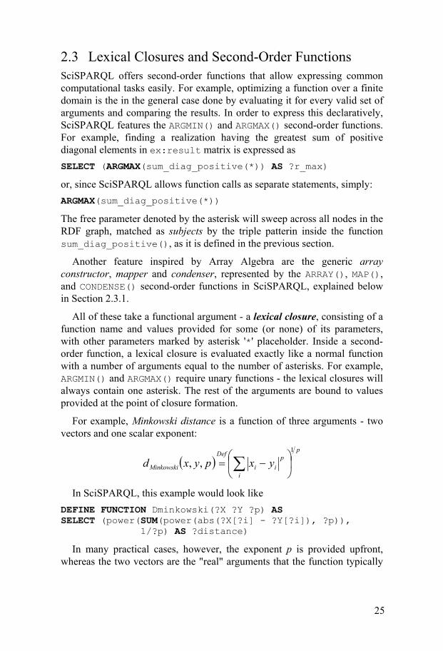
For example, Minkowski distance is a function of three arguments - two vectors and one scalar exponent:

p

i

p

ii

Def

Minkowski yxpyxd1

,,

In SciSPARQL, this example would look like

DEFINE FUNCTION Dminkowski(?X ?Y ?p) AS SELECT (power(SUM(power(abs(?X[?i] - ?Y[?i]), ?p)), 1/?p) AS ?distance)

In many practical cases, however, the exponent p is provided upfront, whereas the two vectors are the "real" arguments that the function typically

25

maps over. For example, Euclidean distance can be defined as a function of two arguments

2,,, yxdyxd Minkowski

Def

Euclid

Lexical closures eliminate the need of defining and naming single-use functions. So, instead of separately defining, and then providing dEuclid as a functional argument, one could directly use Dminkowski(*, *, 2) as an equivalent binary function.

2.3.1 Array Algebra Second-order Functions An array constructor returns an array of given type and shape. It expects a unary function (or closure) that takes a vector of logical subscripts as a single argument, and computes the array elements:

ARRAY(type, shape, mapper)

An array mapper maps over a collection of aligned arrays. It returns a new array of given type aligned to that collection. It expects an n-ary function (or closure) that is mapped over the respective elements of the given arrays:

1n

MAP(type, mapper, v1, ..., vn)

An array condenser computes an intra-array aggregate value applying a given aggregate operation to all array elements. No particular order is guaranteed; hence the aggregate operation (represented by a binary function or closure) is required to be commutative and have identical domain and range.

CONDENSE(op, v)

An additional unary filter function, if provided, will be applied first, in order to select elements based on their value:

CONDENSE(op, v, filter)

Intra-array aggregate functions like array_sum(), array_avg(), etc. are equivalent to particular condenser calls.

2.4 Foreign Functions As mentioned above, a typical scientific or engineering data processing task involves both data retrieval and extensive computations. While the querying capabilities of SciSPARQL address the data retrieval task in a more general and expressive way than generally seen in manually written programs,

26

calling various computational routines should stay similar to the way it is normally done in C, Python, or Matlab. At the same time, the query optimizer should retain the freedom to call the filtering and post-procesing tasks in the optimal order, based on the cost and cardinality estimates, as explained below.

For this purpose, SciSPARQL offers a mechanism for extensibility with foreign functions. While being implemented in algorithmic languages (currently C/C++, Java, Lisp, Python, or Matlab), these functions are used directly in a query: the SELECT clause typically contains the post-processing expressions, and FILTER/HAVING clauses contain the expressions that filter the potential query solutions. In the same way as functional views, foreign functions can be used to form lexical closures and be passed to second-order functions, as explained in Section 2.3.

The process of introducing a foreign function to SciSPARQL typically involves three steps: providing a function implementation or a wrapper for a library

function, with the signature (header) compatible to SciSPARQL, linking the implementation to SSDM (mechanisms for different

languages vary), and defining the new SciSPARQL function using the DEFINE FUNCTION

statement, optionally providing cost and cardinality estimates.

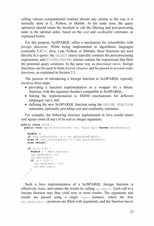
For example, the following function implemented in Java would return real square roots (if any) of its real or integer argument:

public class MyLib { public void sqroot(CallContext cxt, Tuple tpl) throws AmosException { double x; if (tpl.isDouble(0)) x = tpl.getDoubleElem(0); else if (tpl.isInteger(0)) x = tpl.getIntElem(0); else return; if (x >= 0.0) { double r = Math.sqrt(x); tpl.setElem(1, r); cx if (x > 0.0) {

t.emit(tpl);

tpl.setElem(1, -r); cxt.emit(tpl); } } } }

Such a Java implementation of a SciSPARQL foreign function is effectively static, and returns the results by calling cxt.emit(). Each call to a foreign function may thus yield zero or more results. The arguments and results are passed using a single Tuple instance, where the first tpl.getArity()-1 positions are filled with arguments, and the function has to

27

fill the last one with its result before emitting. In all these respects, C/C++ and Lisp interfaces are similar and offer the same degree of flexibility, while Python and Matlab interfaces offer a direct mapping of SciSPARQL function arguments to those of the implementing function.

Since SciSPARQL is a dynamically typed language, in all cases a runtime type check is necessary. By convention, as explained in Section 1.6, a runtime error is not an exception, but instead the absense of any emitted result. An invalid value passed to a filter or postprocessing function is equivalent, e.g., to an unmatched triple pattern, simply resulting in a discarded solution. Hence, AmosException is reserved only for so-called internal errors, and cannot be thrown because of the wrong input.

Linking of such a Java implementation is achieved by including the bytecode for MyLib into Java's CLASSPATH when running SSDM under JVM. In case of Python, the source code needs to be placed in PYTHONPATH. In case of C/C++, linking involves compiling a separate dynamic-link library, and dynamically loading it into SSDM process, by issuing LOAD_EXTENSION('mylib'), referring to mylib.dll in Windows path or libmylib.so in Linux library path. Lisp source files are loaded in a similar way using SOURCE_LISP(). Matlab foreign functions require no additional linking, since they are available as callbacks from the SSDM process embedded into Matlab.

Finally, the SciSPARQL definition of sqroot() would look like:

DEFINE FUNCTION sqroot(?x) AS JAVA 'MyLib/sqroot' COST 4 FANOUT 1

Here the optional COST and FANOUT parts specify the cost and cardinality estimates. Even very rough estimates would help the optimizer much better than the absence of any. By convention, the unit cost corresponds to a simple arithmetic operation like + or * over scalar operands. FANOUT specifies the average amount of results emitted per function call - in our case it averages to one (i.e. zero for negative arguments and two for positive).

Whenever possible, the users are encouraged to provide foreign functions as multidirectional so that the optimizer might choose to compute the function arguments if the result happens to be bound eariler. Such definitions are made by specifying the alternative binding patterns as strings composed of 'b' for bound and 'f' for free (or, respectively, '-' and '+'), and providing an implementation for each. For example, if a similar

28

implementation square() is defined7 in MyLib Java class, the multidirectional definition would be:

DEFINE FUNCTION sqroot(?x) AS FOR 'bf' JAVA 'MyLib/sqroot' COST 4 FANOUT 1 FOR 'fb' JAVA 'MyLib/square' COST 1 FANOUT 1

In this example we have shown a function dealing with simple types, like Double and Integer, wich are mapped to Java's (or other languages') native type system. Since the RDF with Arrays data model introduces RDF-specific types, like langage- and locale-annotated strings, typed literals, URIs, and most notably, Numeric Multidimensional Arrays; each language interface provides the additional classes for each of these. For example, a Java implementation would use UString, TypedRDF, URI, and NMA (array) wrapper classes defined in ssdm package. Each of them provides constructors and field accessors to facilitate the native data processing.

The complete extensibility interface documentation for each language is a part of the SciSPARQL User Manual.

2.5 Calling SciSPARQL from Algorithmic Languages SciSPARQL queries can easily be incorporated into traditional algorithmic programs - this appoach would be somewhat opposite to the one descibed in the previous section. However, both approaches are typically combined in sufficiently complex real-life applications. Declarative SciSPARQL queries may thus be embedded in traditional data processing routines, which might include data acquisition, logging, visualisation, user interactions, or feedback loops in a control system.

The process of calling SciSPARQL queries (or SciSPARQL functions as parameterized queries - see Section 2.2) relies on the concepts of connection and scan (result set), and involves the following steps:

establishing a connection to SSDM server, passing a query string (or a function name and actual arguments) to

the server, and retrieving a scan, iterating through the scan, effectively running the query execution

plan just enough to retrieve yet another result, closing the scan, closing the connection.

7 The implementation of square() should be aware of the binding pattern it is called

with, as it has to retrieve its de-facto argument from position 1 and write its result into position 0. For this reason, sqroot_fb() might be a better name for such implementation.

29

30

An important scalability feature is the lazy evaulation of SciSPARQL queries. A query does not have to be executed in its entirety in order to obtain a scan. Instead, it is the scan object that calls back SSDM in order to advance the query execution on demand. After retrieving each result, the application program is free close the scan, thus terminating the query - a feature more powerful than LIMIT clause inside a query, as any application logic can be involved. However, providing the LIMIT clause is still a good practice when the number of results to retrieve is fixed - this provides more freedom to the optimizer.

Usage of embedded SciSPARQL queries, in the context of Matlab integration, is demonstrated here. Java, C/C++, and Python programs may use the respective APIs, implementing the Connection and Scan classes.