1

PUBLIC SPENDING IN DEVELOPING COUNTRIES:

TRENDS, DETERMINATION, AND IMPACT

Shenggen Fan and Anuja Saurkar1

1. INTRODUCTION

Government spending patterns in developing countries have changed dramatically over the last several decades. Thus, it is important to monitor trends in the levels and composition of government expenditures, and to assess the causes of change over time. It is even more important to analyze the relative contribution of various expenditures to production growth and poverty reduction, as this will provide important information for more efficient targeting of these limited and often declining financial resources in the future. There have been numerous studies on the role of government spending in the long-term growth of national economies (Aschauer 1989; Barro 1990; Tanzi and Zee 1997). These studies found conflicting results about the effects of government spending on economic growth. Barro was among the first to formally endogenize government spending in a growth model and to analyze the relationship between size of government and rates of growth and saving. He concluded that an increase in resources devoted to non-productive (but possibly utility-enhancing) government services is associated with lower per capita growth. Tanzi and Zee also found no relationship between government size and economic growth. On the other hand, Aschauer’s empirical results indicate that non-military public capital stock is substantially more important in determining productivity than is the flow of non-military or military spending, that military capital bears little relation to productivity, and that the basic stock of infrastructure of streets, highways, airports, mass transit, sewers, and water systems has most explanatory power for productivity. Many studies also attempted to link government spending to agricultural growth and poverty reduction (Elias 1985; Fan et al. 2000; Fan et al. 2004; Fan and Pardey 1998, and Lopez 2005). Most of these studies found that government spending contributed to agricultural production growth and poverty reduction, but different types of spending may have differential effects on growth and poverty reduction. The purpose of this study is to review and analyze the trends and causes of change in government expenditures and their compositions in the developing world, and to develop an analytical framework for determining differential impacts of various government expenditures on economic growth. We first review trends in and the composition of government expenditures across developing regions of Africa, Asia, and Latin America. We then model determinants of composition of government expenditures. Next, we model effects of government expenditures on gross domestic product (GDP) growth by estimating a GDP function and estimate the impact of various public capitals on agricultural GDP growth. We conclude with the study’s major findings.

1 The authors thank Annie White and Neetha Rao for able research assistance.

2

2. GOVERNMENT SPENDING: TRENDS, SIZE, AND COMPOSITION

Measures Total expenditure is broken down into various sectors following the International Monetary Fund’s Government Finance Statistics (GFS) Yearbook sectors. This study concentrates on six sectors, namely agriculture, defense, education, health, social security, and transportation and communication. Appendix Table 2.1 provides further description on these sectoral definitions.

To convert expenditures, denominated in current local currencies, into international dollar aggregates expressed in base year (2000), prices were first deflated from current local currency expenditures to a set of base year prices using each country’s implicit GDP deflator. We then used 2000 exchange rates measured in 2000 purchasing power parity reported by the World Bank Indicators (2006) to convert local currency expenditures measured in terms of 2000 prices into a value aggregate expressed in terms of 2000 international dollars.

We included 44 developing countries from three regions in our analysis, partly reflecting the availability of data and partly because these countries are important in their own right while representing broader rural development throughout all developing countries. The 17 countries included for Africa are Botswana, Burkina Faso, Cameroon, Côte D’Ivoire, Egypt, Ethiopia, Ghana, Kenya, Malawi, Mali, Morocco, Nigeria, Togo, Tunisia, Uganda, Zambia, and Zimbabwe. We included 11 countries from Asia: Bangladesh, China, India, Indonesia, Korea, Malaysia, Myanmar, Nepal, Philippines, Sri Lanka, and Thailand. For Latin America, we included 16 countries: Argentina, Belize, Bolivia, Brazil, Chile, Colombia, Costa Rica, Dominican Republic, Ecuador, El Salvador, Guatemala, Mexico, Panama, Paraguay, Uruguay, and Venezuela. In 2002, these countries account for more than 80% of both total GDP and agricultural GDP in developing countries.

The data coverage for the Asian countries includes both central and sub-national expenditure in the GFS. Many of the African countries have minimal local government expenditures or lack sub-national government entities. In addition, expenditures by the local governments are central government transfers that are reflected in the central government budget. However some Latin America countries have made significant decentralization efforts in the recent decades. These efforts have been captured in the data for the large countries such as Argentina, Bolivia, Chile, Colombia, Mexico and Paraguay. But for smaller countries in the region, some of the local government expenditures may have not been captured by the IMF dataset. Budgetary support on social sectors to local NGOs is not captured by the data.

Finally, we geometrically extrapolated data for countries whose values were missing to ensure continuity of data (see Appendix Table 2.2 for a summary of these extrapolations by country).

Size of Government Spending Over the past two decades, total government expenditures, in the 44 developing countries considered in this study, experienced overall growth. During the 1980s, expenditures increased from $993 billion in 1980 to $1,595 billion in 1990, with an annual growth rate of 4.8 percent

3

(Table 2.1). In the 1990s, governments increased their spending power by 5.6 percent per year. By 2000, total government expenditures increased to $2,748. billion. They further reached $3,347.6 billion in 2002. Therefore, we have seen accelerated growth in government expenditures in developing countries.

However, amongst developing countries, regional deviations from these averages were quite marked. Across all regions, Asia experienced the most rapid growth, while Africa and Latin America increased at a much slower pace. In fact, most of the increase in total government expenditures came from Asia, accounting for 67 percent of total expenditures in 2002, up from 50 percent in 1980. This is due to the fact that most Asian countries experienced rapid growth in per capita GDP. With the exception of Sri Lanka and Myanmar, all countries in the region at least doubled their total expenditures for the period 1980–2002. Republic of Korea and Bangladesh had the most rapid growth over 1980–2002, followed by India and Thailand.

For African countries, expenditures grew at 3.8 percent over 1980–2002. Growth was much slower in the 1980s, at 2.92 percent per annum. In fact, there was a brief contraction after 1982, and it was not until 1986 that total government expenditures recovered to 1982 levels, when many African countries implemented macroeconomic structural adjustments. However, during the 1990s African countries gained momentum in expanding government expenditures, growing at 4.8 percent per annum. Botswana had the most rapid growth, mainly due to the outstanding performance of its national economy: more than 10 percent growth per annum during 1980–2002.

Latin American countries had the slowest growth in spending between 1980 and 2002. The share of the 16 countries of the total expenditure reduced from 38% in 1980 to 26% in 2000. The growth rate in the 1980 was 4% and much less in the 1990s with 2.29%. Many countries in the region including large ones like Argentina and Brazil were faced with structural adjustment programs which led lower spending in the social sectors and overall government expenditure.

Total government expenditure as a percentage of GDP measures the amount a country spends relative to the size of its economy. For countries in this study, the percentage increased from 19 percent in 1980 to 22 percent in 2002. 2 On average, developing countries spend much less than developed countries. For example, total government outlays as a percentage of GDP in Organization for Economic Cooperation and Development (OECD) countries range from 27 percent in 1960 to 48 percent in 1996 (Gwartney et al 1998), compared to 13–35 percent in most developing countries (For detailed information on each country, refer to Appendix Table 2.3).

For Asia, the percentage increased from 19 percent in 1980 to 20 percent in 2002. There is a strong correlation between the level of economic development and government spending power in this region, with the exception of Sri Lanka. In 2002, Myanmar spent the least, only 8 percent of its GDP, while the rest of the Asian countries spent 14–25 percent of their GDP. India has been spending 17 percent of its GDP since it liberalized its economy in the 1990s whereas China has accelerated its spending since 2000. Thailand has also accelerated its spending to a quarter of its GDP.

2 Since the weighted commonly calculated at the regional and global level may bias towards large countries, we also report unweighted average at the regional and global levels.

4

Surprisingly, among the three regions, Africa spent the most as a percentage of GDP. Government spending as a percentage of GDP was roughly 27–34 percent over the last two decades, almost 10 percentage points higher than Asia and Latin America. Among all countries in the region, Botswana, Nigeria, Malawi, Ethiopia, Tunisia, and Zimbabwe were among the largest spenders, often spending 35 - 67 percent of their GDP. Uganda and Cote d’Ivoire spent only a fraction as much, about 3-16 percent, the least among African countries in our study.

Latin America experienced even more of an erratic spending pattern. The percentage increased at a rate of 2–3 percent per year until 1986, then declined thereafter at a rate of 1–2 percent per year from 1987 to 1991. After 1992, the percentage began another upward trend. For the region, the percentage averaged 25 percent in 2002, slightly higher than Asian countries. Uruguay spent over 30 percent, while Guatemala spent roughly 14 percent equivalent to their respective GDPs.

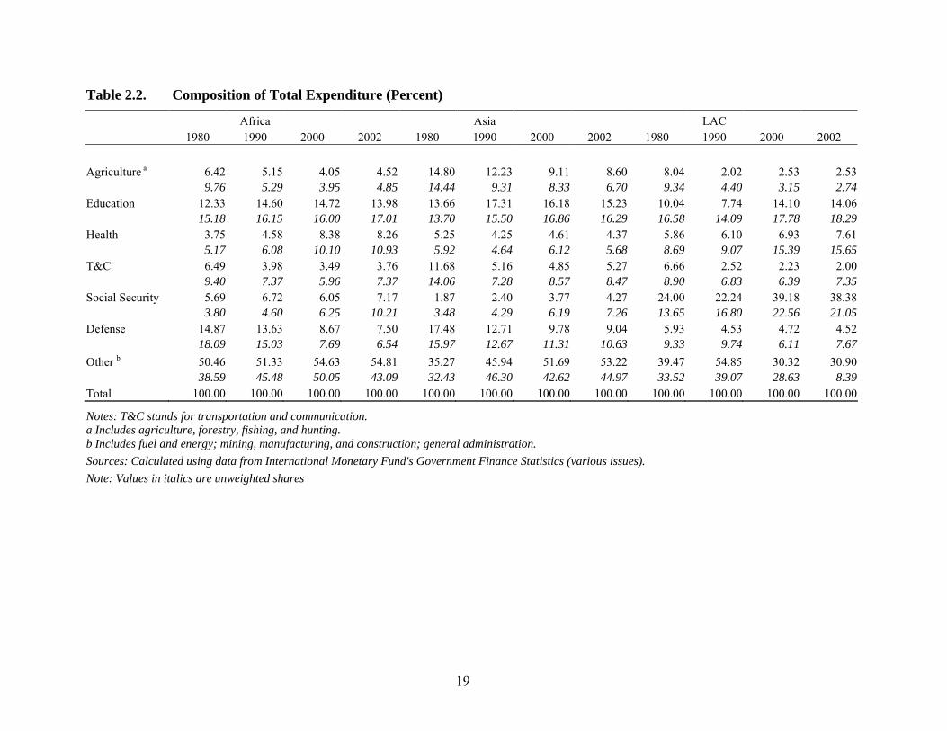
Composition of Government Spending Equally important is the composition of government expenditures, which reflects government spending priorities. The composition of total expenditure across regions reveals many differences (Table 2.2).3

The top three expenditures for Africa in 2002 were education, defense, and health. Although education expenditure was the largest (14 percent), the percentage is smaller than in Asia and comparable to Latin America. Defense accounted for 8 percent of total government expenditures in the region, similar to Asia. African countries spent 8 percent of total government expenditures on health. A discouraging trend is that African countries and Latin America spent very little on transportation and telecommunication. Africa’s share in total government expenditures gradually declined from 6.4 percent in 1980 to 3.8 percent in 2002. The decline is much sharper in the case of Latin America from 6.6 percent to 2 percent from 1980 to 2002.

Education spending was the largest among all government expenditures in Asia, accounting for 16 percent in 2002. It is not surprising that Asia has the highest quality of human capital among regions. Defense and agriculture spending ranked second and third, accounting for 9 percent each, of total government expenditures in 2002, reduced from 18 percent and 15 percent, respectively, in 1980.

Governments in Asia slightly reduced their spending in health as a share of total government spending from 1980 to 2002. This indicates that as the economy continues to recover from the 1997 Asian Crisis, governments in the region may be spending less on health, though is much needed to protect disadvantaged groups. Although defense spending declined from 18 percent in 1980 to 9 percent in 2002, the percentage was still high compared to Latin America, which spent 4.5 percent on defense, and was substantially higher than the region’s spending on infrastructure, social security, and health.

For Latin America, social security spending ranked at the top of all government expenditure items, indicating that higher income inequality among population groups in the

3 Comparison is made across six sectors, namely agriculture, education, health, defense, social security, and transportation and communication. Other sectors, such as mining, manufacturing and construction, fuel and energy, and general administration, are not included in our analysis and are collectively termed “other” expenditures.

5

region may call for government intervention. In addition, Latin America spent 10-14 percent of total expenditure on education between 1980 and 2002. Agricultural expenditure accounted for a small fraction of total government expenditures (2.5 percent), mainly due to the small share of agriculture in national GDP.

Other expenditures (which include government spending in fuel and energy, mining, manufacturing and construction, and general administration) accounted for roughly 50 percent of total government spending in Africa over 1980–2002. For Asia, the share of this type of expenditures increased from 35 percent in 1980 to 53 percent in 2002. For Latin America, it also accounted for more than 31 percent of total government spending in 2002. Most of these expenditures were either government subsidies or expenses relating to general administration. The large and increasing share of these expenditures may have competed with more productive spending items such as agriculture, education, and infrastructure.

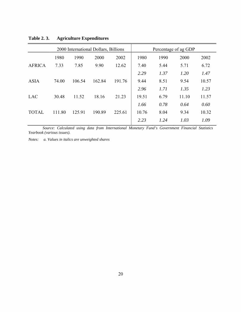
Agricultural Spending Agriculture is the largest sector in many developing countries in terms of their shares in GDP and employment. More importantly, the majority of the world’s poor live in rural areas and depend on agriculture for their livelihood. Sustainable agricultural development is therefore imperative in the quest for development. Therefore, agricultural expenditure is one of the most important government instruments for promoting economic growth and alleviating poverty in rural areas of developing countries. Agriculture expenditures increased at an annual growth rate of 3.2 percent between 1980 and 2002 (Table 2.3). During the same period of time, rural population grew at approximately 1 percent per year, and agricultural GDP by 4.2 percent. Therefore, we saw a slight increase in agricultural expenditures per capita of rural population, and a decrease of agricultural expenditures per unit of agricultural GDP.

In Africa, government expenditure on agriculture increased gradually at an annual rate of 2.5 percent. Agricultural expenditures in Asia more than doubled in the past two decades, with an annual growth rate of 4.4 percent, the highest growth among the three regions. Latin America was the only region that reduced its spending in agriculture, with an annual reduction of 1.6 percent. Six out of the 16 Latin American countries included in this study reduced their government expenditures in agriculture.

Agriculture expenditure as a percentage of agriculture GDP, measures government spending on agriculture relative to the size of the sector. Compared to developed countries, agricultural spending as a percentage of agricultural GDP is extremely low in developing countries. The former usually has more than 20 percent, while the latter averages less than 10 percent. In Africa, agriculture expenditure as a percentage of agricultural GDP remained at relatively similar levels (5.4–7.4 percent) throughout the study period. About half of African countries decreased agriculture expenditure relative to agricultural GDP. Asia’s performance was much higher to that of Africa, as its percentage remained constant at 8.5-10.5 percent. For Latin America, agricultural spending as a percentage of agricultural GDP decreased from 19.5 percent in 1980 to 11.5 in 2002.

Among all types of agricultural expenditures, agricultural research and development is the most crucial to growth in agricultural and food production. Beintema and Stads (2004) show that agricultural research and development (R&D) expenditures as a percentage of agricultural

6

GDP saw a relatively stable increase in the last three decades. For example, in 2000, the share of agricultural R&D expenditure in agricultural GDP in Africa and Asia was between 0.5–0.9 percent, and Latin America’s share was 0.98 percent. These rates are relatively low compared to 2–3 percent in developed countries.

3. DETERMINATION OF GOVERNMENT EXPENDITURES

In this section, we attempt to gain insights by modeling government spending patterns. Determination of total government spending and its patterns is complex and may include many factors, such as fiscal conditions and political, cultural and economic factors.

In the 19 the century, economists generally advocated a state with minimal economic functions, or the so-called Laissez-Faire. This was a response to failures in the 18th century due to heavy government distortions (Tanzi and Schuknecht, 2000). After World War I, the perception about the role of government changed again due to the influence of Keynes who argued that the government still had many things to do that were not being done. In response to the Great Depression, the United States introduced major public expenditure programs to generate public goods and create employment. This period continued up to the 1980s. For OECD countries, percentages of total government expenditures in total GDP increased sharply from 13.1% in 1913, to 23.8% in 1937, 28% in 1960, and 41.9% in 1980. During the 1980s and 1990s, skepticism about the large size of the government grew increasingly over time due to government failures to use public spending to achieve higher growth and better income distribution outcome. But for many OECD countries, the size of government continued to grow, but in a much slower pace (for example, government spending as a percentage of GDP grew from 43.1% in 1980 to 44.8% in 1990 and 45.6% in 1996).

More complicated is the determination of the composition of government spending. Rent seeking behavior, economic and political structures, economic development level among others are all important in this process. The government can act as a social planner when allocating public spending. The social planner determines the optimal allocation by maximizing a weighted social welfare function. Under this approach, the government maximizes a utility function⎯ defined over a set of public services consumed by the individuals or electorate⎯subject to a budget constraint equal to the sum of public service expenditures (Deacon 1978).

Rent seeking behavior has been an increasingly important subject under study in determining the allocation of government spending. Specifically, the distribution of potential individual beneficiaries of rents, the number of groups competing, the rule used to distribute private good transfers within groups, and the individual valuation of the local public good shape public spending patterns (Nitzan 1994). Public choice economics provides a theoretical basis for studying the role of political processes in the level and composition of public expenditures. Sass (1991), for example, constructed a model of municipal government choice based on the constitutional choice model of Buchanan and Tullock (1962) to analyze the impact of differing government structures on two categories of public spending: educational and non-educational

7

expenditures.4 The results suggest that voter preferences appear not only determine the level of municipal expenditures but the structure of local governments as well.

Ideological difference between groups and the parties that represent these groups matter suggesting that lower income groups favor a large and active state while upper income groups aim at minimizing the role of the state. Cusack (1997) analyzed the role of ideologically based partisan preferences in influencing public spending levels in a regression analysis using data from 15 OECD countries over the 1950-1989 period. To account for the impact of partisan politics, the author constructed two indices with a similar structure to represent government and electorate ideological preferences on left-right scale. These indices represent the ideological preference of the government party that shapes the preferences for more or less spending. The results support the partisan politics model in that the left increases the size of the public sector while the right reduces it.

While political factors influence the level and structure of public expenditures, economic and demographic factors are also important to consider. For example, Rodrik (1998) relates the degree of openness of the economy to the level of government spending. Demographic variables also influence the level and composition of public spending as an aging population demand greater spending on health, housing, and social security (Feldstein 1996). Similarly, a rise in the proportion young people affects the demand for education spending (Marlow and Shiers 1999). Structural differences, such as the degree of urbanization or population density, also affect government spending (Dao 1995). Dao found that population density has a positive influence on per capita expenditures on housing, social security and welfare, and education in developed economies. On the other hand, urbanization helps explain variations in per capita expenditures on social security and welfare among developing countries. It is not our objective in this paper to model the political and cultural factors. Our major purpose is to analyze how the structural adjustment programs have affected the spending pattern. However, in order to avoid the bias due to the omission of these variables, we use country dummies to control for these effects assuming that these factors have not changed over time.

TOTAL GOVERNMENT SPENDING

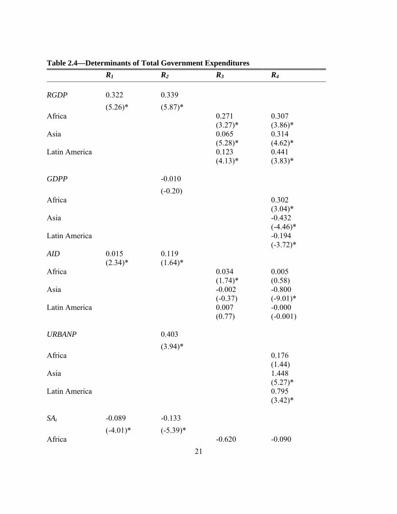
When we control for political, social and cultural factors, how much a government can spend depends on its revenues and its ability to borrow from international and domestic sources. For many small developing countries, international aid also has become a significant source of government expenditures. In Uganda, Tanzania and Ghana, total foreign aid accounts for 15-30% of total GDP (World Bank, 2006). The relative importance of these factors changes over time. In particular, when a government introduces budget cuts under the aegis of macroeconomic reforms and adjustments, spending patterns are likely to be affected. We use the following specification to model changes in government expenditures.

GEPGDPt = f(RGDPt, AIDt, SAt,, Xt) (1) 4 Buchanan and Tullock’s (1962) constitutional choice model shows that individuals select the collective choice mechanism, which minimizes the costs associated with group decision-making. The optimal form of government involves a tradeoff between external and internal or decision-making costs.

8

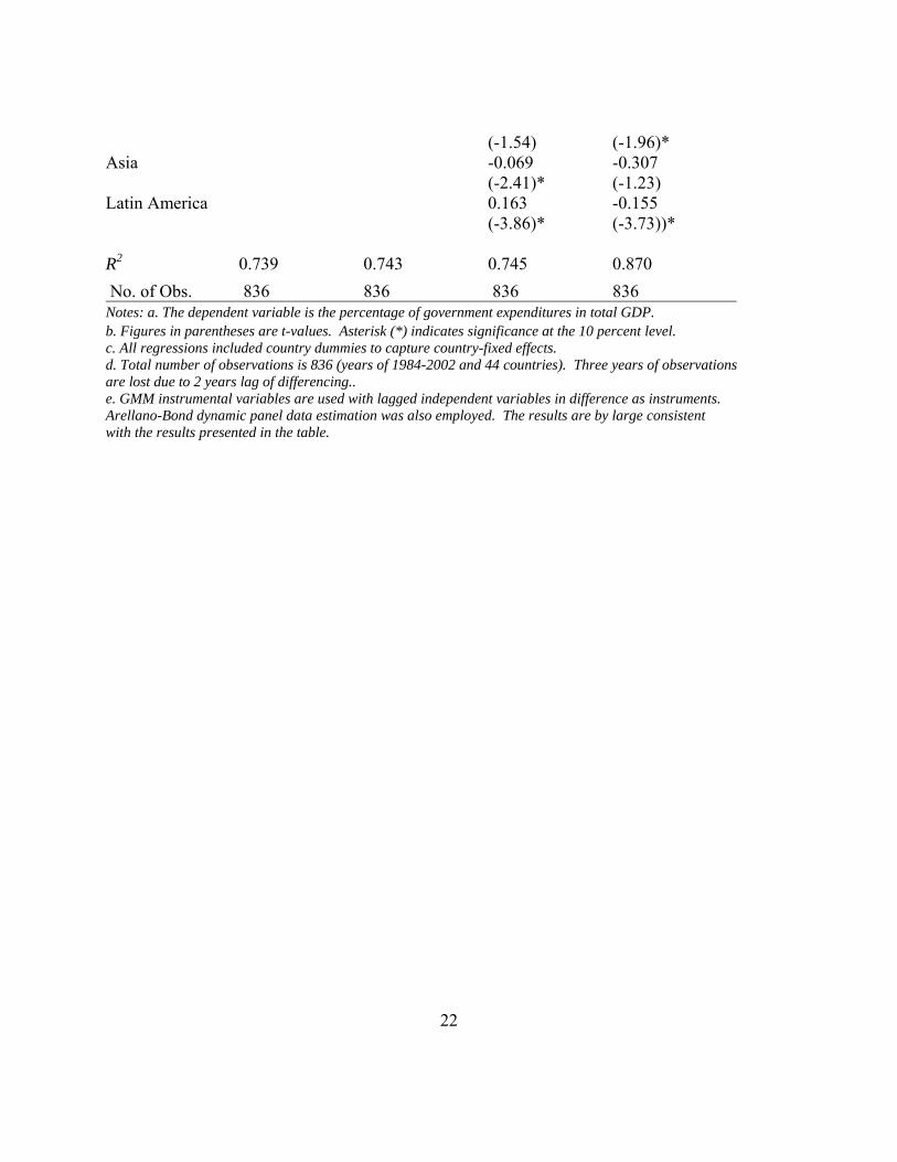
Where GEPGDPt is government expenditure as a percentage of GDP and RGDPt is government revenue as a percentage of GDP. AIDt is total aid received by the country measured as a percentage of GDP. The variable SAt is a dummy variable that is equal to 1 when macroeconomic adjustments are implemented and equal to 0 otherwise.5 Apart from revenue and structural adjustment variables, Xt captures the effect of other factors on government spending. Since it is difficult to quantify them, we use both year and country dummies to proxy these factors. Since revenue, aid and structural adjustment programs can also be the function of government revenue, there may exist a reverse causality. The ordinary least square estimation technique will lead to biased estimation. To avoid the potential endogeneity problem of the independent variables, the GMM instrumental variable approach is used. Two years lagged independent variables in difference are used as instruments. Another estimation issue that may cause spurious regressions is possible existence of unit roots or nonstationarity of variables included in the analysis. However, when the number of cross-sectional units (N) is much larger than the number of time periods (T), the nonstationarity problem commonly seen in time-series data can be attenuated (Holtz-Eakin et al., 1988). Just to ensure that there is no unit root problem in our panel dataset, we used Dickey-Fuller approach to conduct various tests. When we conduct tests country by country, we found that for government revenues, expenditures, foreign aid, and agricultural expenditures, the hypothesis of unit root is rejected for most of the countries. For GDP and agricultural GDP, however, hypothesis is rejected for only one third of the countries. However, when we pool all countries together, all variables do not show existence of unit root when country dummies are added or both country and year dummies are added. When dummies are not added, only GDP and agricultural GDP show an existence of unit root. Therefore, to avoid the problem of unit root, at least country dummies must be added. More details on the estimation procedures in a panel dataset are attached as 1. Regression results are presented in Table 2.4. We have four different specifications. Regression 1 includes only revenue and structural adjustment program variables. In regression 2, we added GDP per capita (GDPPt), and urbanization (URBANPt) variables. These two variables illustrate how economic development levels and demographic shifts affect government spending. Regressions 3 and 4 are results from variable coefficient models in which all parameters in the regressions vary by region. This is because determination of government expenditures may differ by region even after controlling for all variables in the equations. Results in regression 1 indicate that government expenditure is largely determined by revenue and structural adjustment. The latter was found to reduce government expenditure (the coefficient of the structural adjustment variables is negative and statistically significant). Regression 2 shows that after controlling for GDP per capita and for urbanization, the structural adjustment program variable is still statistically significant and negative. When we break our analysis into regions, we find that for all regions, structural adjustments reduced government spending. All these coefficients are statistically significant except for those of Africa when per GDP and urbanization are not controlled for and those for Asia when these two variables are

5 The initiation years of structural programs by country were reported by IMF (Barro and Lee 2003). It is defined as the first year when the IMF implemented its structural adjustment program loans.

9

controlled for. This finding is by large in consistent with the objective of the structural programs of cutting down the government spending.6

COMPOSITION OF SPENDING

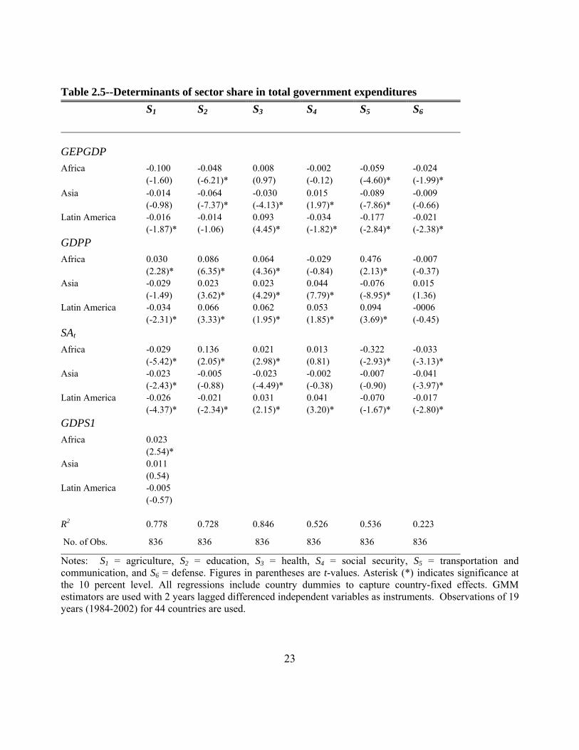
Some studies have analyzed the impact of composition of government spending on economic growth (Devarajan, Swaroop, and Zou 1996), but few have modeled the determination of composition. Understanding why certain countries spend more on one sector than others will help developing countries reallocate government resources to the most productive sector by focusing on major forces behind existing patterns. The composition of government spending is modeled in the following specification:

Si,t = g(GEPGDPt, GDPPt, SAPt, Zi,t) (2) where Si,t is the share of ith sector7 in total government expenditure, GEPGDt is government expenditure as a percentage of GDP, GDPPt is per capita GDP, and Zi,t comprises other factors that may affect government spending in the sector. Again, we use year and country dummies to proxy for Z and to control for other factors excluded from the equation. Similar to equation 1, we also use GMM instrumental estimator for estimating the share equations. Regression results are presented in Table 2.5. For all regressions, we disaggregated our analysis into regions. As total government expenditures increase, the share of agriculture expenditure (S1) declines in all regions although the coefficient is statistically significant only in Latin America. The share of the agriculture sector in total GDP (GDPS1) is not statistically correlated with government expenditure shares in agriculture in Asia and Latin America. In Africa, as the share of the agricultural sector increases, the share of the government spending on agriculture also increases. The most important finding is that structural adjustments reduced government expenditure shares in the agriculture sector in all regions. Since agricultural spending is the most pro-poor and contributes to overall economic growth, the cut in agricultural spending may adversely affect the poor and overall economic growth. Results for S2 (education sector) indicate that as a country becomes richer, the share of education expenditures becomes larger, evidenced by positive and statistically significant coefficients of the per capita GDP variable in the education share equation. Structural adjustments increased spending share on education in Africa, but reduced share in Latin America. It had no statistically significant impact on education spending in Asia. Similar to education, as countries become richer, they tend to spend more on health. Coefficients of per capita GDP are all positive and significant. The structural adjustment

6 Barro and Lee (2003) found no significant effects of SAPs on government consumption. 7 where S1 = agriculture, S2 = education, S3 = health, S4 = social security, S5 = transportation and communication, and S6 = defense.

10

programs increased spending on health in Africa and Latin America, but reduced the share in Asia. Results from S4 show that the share of social security in total government expenditures in Africa has generally no relationship with their economic development level (per capita GDP). By contrast, as economy expands, governments tend to spend more on social security in Asia and Latin America. The structural adjustment programs increased social security spending in Latin America, but had no statistically significant impact in Asia and Africa. Structural adjustments had an adverse impact on government spending on infrastructure across all regions, although they are statistically insignificant in Asia (regression S5 in Table 2.5). This implies that governments may have reduced infrastructure investment during macroeconomic structural adjustment programs, particularly in Africa and Latin America. The relationship between government spending on defense and economic development level is not statistically significant. As government revenues increase, developing countries tend to reduce their shares on defense. Structural adjustment programs have reduced government spending share on defense in all regions.

4. IMPACT OF GOVERNMENT SPENDING ON GROWTH

Many studies have analyzed how government expenditures contribute to economic growth (Barro 1990; Kelly 1997). However, they focused on the impact of total government expenditures and overall GDP growth. Very few studies attempted to link different types of government spending to growth, and even fewer attempted to analyze the impact of government spending at the sector level. In this section, we first model the impact of different types of government spending on overall GDP growth, and then analyze the effect of agricultural spending on agricultural GDP.

SPENDING AND OVERALL GDP GROWTH

We estimate a production function with national GDP as the dependent variable, and labor, capital investment, and various government expenditures as independent variables.

GDPt = h(LABORt, Kt, KGE i,t, SAt, Wt) (3) Where GDPt is GDP at year t, LABORt and Kt are labor and private capital inputs at year t, and KGEi,t is capital stock constructed from current and past government spending in the ith

sector with KAGEXPt representing government stock in the agricultural sector, KEDEXPt representing the education sector, KHEXPt representing the health sector, KTCEXPt representing the transportation and telecommunication sector, KSSEXPt representing the social security sector, and KDEXPt representing the defense sector. Usually this stock cannot be observed directly, so it serves more as a part of the conceptual apparatus than an empirical tool. To construct a capital stock series from data on capital formation, we used the following procedure:

11

1-tK)δ(1−+= tt IK (4) Where Kt is the capital stock in year t, It is gross capital formation in year t, and δ is the depreciation rate. Since the depreciate rate varies by country, we simply assume a 10 percent depreciation rate for all the countries. To obtain initial values for the capital stock, we used a similar procedure to Kohli (1982):

)rδ(1980

1980 +=

IK (5)

Equation 5 implies that the initial capital stock in 1980 (K1980) is capital investment in 1980 (I1980) divided by the sum of real interest rate (r) and depreciation rate. Impact of structural adjustment programs on economic growth is captured by variable SAt, and other factors not included in the equations are captured through the year and country dummies of Wt.

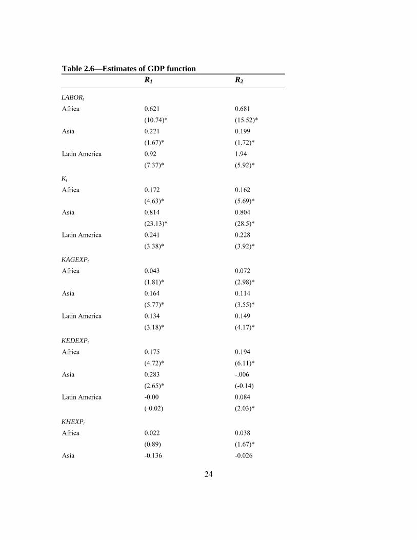
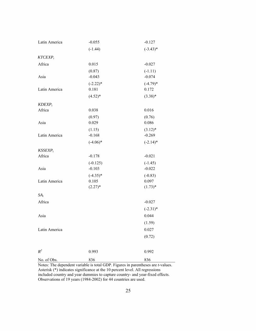
Since government expenditure variables on the right hand side can also be a function of GDP, therefore, there might exist reverse causality. There have been many empirical studies to address these problems by using different econometric techniques, for example, differencing approach and instrumental variables approach. Level-based regressions generally show a much higher return to public capital (either in terms of physical terms such as length of roads or in stock measured in monetary value) than private capital, while difference-based regressions tend to find insignificant or even negative effects. To reconcile this controversy, Zhang and Fan (2004) first apply a system GMM method to empirically test the causal relationship between productivity growth and infrastructure development using the India district level data over 1970 to 1994. The test shows a long-term relationship between these two, therefore calling for a level-based regression. They then proposed an approach to estimate the equation in level but with lagged dependent variables in difference as instruments by using the GMM system estimator, so the long term effects can be estimated while the endogeniety of independent variables can be controlled. They found that infrastructure development in rural roads is productive with a magnitude lying between those obtained from conventional level estimates and differenced estimates. This study uses the similar approach to Zhang and Fan. Two years lag of dependent variables (labor, capital, and various government expenditures) are used as instruments. More years lag can also be used to ensure there is no correlation of lagged independent variables and dependent variables. But more observations will be lost if longer lag differencing is used. For more details, refer to Appendix 1. Results are shown in Table 2.6. Regression 1 (R1) reports results by region when structural adjustment variables SA,t are excluded, while regression 2 (R2) reports those with SA,t included. The labor and capital coefficients are positive and statistically significant for all regions. For government expenditures on agriculture, coefficients are positive and statistically

12

significant in all regions. For education expenditure, the coefficients are also positive and statistically significant in most regions except that for Latin America when the SAP variable is not included and that for Asia when the SAP variable is included. The coefficients for health expenditures are generally not statistically significant except that for Asia when the SAP variable is included and that for Latin America when the SAP variable is included. This may be due to the fact that this variable is highly correlated with the education spending variable.8 The coefficient of social security spending in Africa is not statistically significant regardless whether the SAP variable is included. In Asia, the coefficient is negatively correlated with growth when the SAP variable is not included and becomes insignificant when included. The transportation and communication expenditures did not have a positive and statistically significant impact on economic growth in Africa, but negatively correlated with growth in Asia. In Latin America, the coefficient is positive and statistically significant. Lack of public investment in infrastructure in Africa may fail to show the positive relationship between investment and growth. In Asia, public investment may crowd out private investment in the sector, leading to a negative effect. Defense expenditure had an insignificant impact on growth in Africa and Asia. But in Latin America, it had a very strong negative impact on economic growth. Finally, structural adjustment programs reduced GDP growth in Africa, but statistically insignificant in Asia and Latin America. This effect is additional to the effects through reduced spending in productive sectors such as in agriculture and infrastructure.

AGRICULTURAL SPENDING AND GROWTH IN AGRICULTURE

Since agricultural growth has been one of the most effective ways for poverty reduction through the so-called “trickle-down” process, we estimate the determinants of agricultural growth in developing countries. We pay special attention to how government spending can promote growth in the agricultural sector. We include an explanatory variable in the agricultural production function that measures government expenditures on agriculture to identify output-enhancing effects of public expenditures. The production function to be estimated is specified as: AGOUTt = h(AGLANDt, LABORt, FERTt, TRACTt, ANIMALSt, ROADSt, LITEt, KAGEXPt, Ut) (6) where AGOUTt is agricultural output, the dependent variable; the independent variables are labor (LABORt), land (AGLANDt), fertilizer (FERTt), number of tractors (TRACTt), number of draft animals (ANIMALSt), and public input variables such as road density (ROADSt), literacy rate (LITEt), and an agricultural expenditure capital variable (KAGEXPt). Traditionally, an irrigation variable is also often included. But irrigation is a result of government spending and inclusion of this variable may double count the effects of government spending. The variable Ut is used to capture the other factors not included in the equation, and is proxied by year and country dummies.

8 Indeed, when we aggregate education and health spending together as spending in human capital, coefficients in all regions are statistically significant and positive.

13

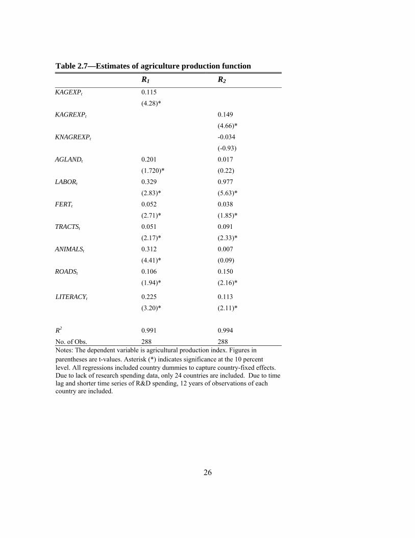
We further disaggregate government expenditures into research (KAGREXPt) and non-research expenditure capitals (NKAGREXPt) to capture separate effects of these two types of expenditures. These capital variables are converted from government expenditures using procedures similar to those described in equations 4 and 5. Output is measured as the agricultural output index reported by Food and Agriculture Organization (FAO), where agriculture is broadly defined to include crop, livestock, forestry, and fishery production. All these variables were incorporated into the estimating equation as indices and in logarithm forms to minimize bias that may arise from using different scales or units of input and output for each country. Two different specifications were estimated, and the results are presented in Table 2.7. The first specification includes conventional inputs such as labor, land, fertilizer, machinery, and draft animals; physical public inputs such as road density, and literacy rate; and a stock variable of total government expenditure on agriculture. The second specification disaggregates total agricultural expenditures into agricultural and non-agricultural research expenditures (total agricultural expenditures net of agricultural research expenditures). Due to the limited number of observations (24), we were unable to conduct this analysis at the regional level. The estimation procedure used is similar to that of the GDP function, i.e., a system GMM estimator with two year lag of independent variables as instruments. The procedure can maintain the long-term relationship and in the meantime to avoid the problem of endogeniety of many righ-hand side variables, particularly those related to government spending. Similar to the results in Table 2.6, total agricultural expenditures had a significant effect on agricultural GDP, as shown in the first regression of Table 2.7. The coefficients for all conventional inputs are statistically significant. Physical public capital inputs, including roads and literacy rate, are all positive and statistically significant. This strongly suggests that broader rural investments in infrastructure and education contributed to agricultural production growth. Disaggregating total agricultural expenditure into research and non-research expenditures reveals an interesting finding: the coefficient for agricultural research is statistically significant and positive while that of non-research spending variable is not statistically significant. The coefficient of research variable in this equation is larger than the coefficient of total agricultural spending variable (includes both research and non research spending) and more statistically significant reported in R1. This is prima facie evidence that productivity-enhancing expenditures, such as agricultural research investments have much larger output-promoting effects than other forms of public spending (including subsidies).

5. MAJOR FINDINGS

In this study, we compiled government expenditures by type across 44 developing countries between 1980 and 2002. We then analyzed trends, determination, and impact of various forms of government spending. The following are the major findings of this study.

14

Total government expenditures for 44 countries included in the study increased over time. Macroeconomic adjustments did indeed reduce the total government spending size. However, they had different consequences for different sectors. For almost all regions, the programs have reduced the spending share on agriculture and on infrastructure. As many studies have shown that, these two productive investments have large returns to GDP growth and poverty reduction, the structural adjustment programs adversely affect these final development indicators by cutting down spending in these two sectors. The performance of government spending in economic growth is mixed. In Africa and Asia, government spending in agriculture and education were particularly strong in promoting economic growth. In Latin America, spending in agriculture, infrastructure and social secutiy had positive growth-promoting effects. Structural adjustment programs had a negative effect on growth in Africa, but no statistically significant effects in Asia and Latin America. Agricultural spending, education, and roads contributed strongly to agricultural growth. Disaggregating total agricultural expenditures into research and non-research spending reveals that research had a larger productivity enhancing impact than non-research spending. Several lessons can be drawn from this study. First, various types of government spending have differential impacts on economic growth, implying greater potential to improve efficiency of government spending by reallocation among sectors. Second, governments should reduce their spending in unproductive sectors such as defense, and curtail excessive subsidies in fertilizer, irrigation, power, and pesticides. Third, all regions should increase spending in agriculture, particularly on production-enhancing investments such as agricultural R&D. This type of spending not only yields high returns to agricultural production, but also has a large impact on poverty reduction since most of the poor still reside in rural areas and their main source of livelihood is agriculture.

15

REFERENCES

Arellano, M. and S. Bond. 1991. Some tests of specification for panel data: Monte Carlo evidence and an application to employment equations. Review of Economic Studies 58: 277-297.

Aschauer, D. 1989. Is public expenditure productive? Journal of Monetary Economics 23: 177–220.

Barro, J. R. 1990. Government spending in a simple model of endogenous growth. Journal of Political Economy 20(2), 221–247.

Barro, R. J., & Lee, J. W. (2003). IMF programs: Who is chosen and what are the effects? Australian National University, Economics RSPAS, Trade and Development

Blundell, Richard and Stephen Bond. 1998. Initial conditions and moment restrictions in dynamic panel data models. Journal of Econometrics 87: 115-143.

Blundell, Richard and Stephen Bond. 1999. GMM estimation with persistent panel data: An application to production functions. Working Paper Series No. W99/4. Institute for Fiscal Studies.

Buchanan, J. and G. Tullock. 1962. The calculus of consent: a logical foundation of constitutional democracy. University of Michigan Press: Ann Arbor.

Canning, David. 1999. Infrastructure’s contribution to aggregate output. Policy Research Working Paper 2246, World Bank.

Cusack, T.R. 1997. Partisan politics and public finance: changes in public spending in the industrialized democracies, 1955-1989. Public Choice vol 91:375-95.

Dao, M.Q. 1995. Determinants of government expenditures: new evidence from disaggregative data. Oxford Bulletin of Economics and Statistics vol. 57:67-76.

Devarajan S., V. Swaroop, and H. Zou. 1997. The composition of public expenditure and

economic growth. Journal of Monetary Economics 37.

Deacon, R.T. (1978). A demand model for the local public sector. Review of Economics and Statistics vol 60: 1980-202.

Elias, V. 1985. Government expenditures on agriculture and agricultural growth in Latin

America. Research Report 50. Washington, D.C.: International Food Policy Research Institute.

Fan, S., P. Hazell, and S. Thorat. 2000. Government spending, agricultural growth and poverty in rural India. American Journal of Agricultural Economics 82(4).

16

Fan, Shenggen, L. Zhang and X. Zhang. 2004. Investment, Reforms and Poverty in Rural China, Economic Development and Cultural Change, Vol. 52, No. 2, pp. 395-422.

Fan, S., and P. Pardey. 1998. Government spending on Asian agriculture: Trends and production consequence. In Agricultural public finance policy in Asia. Tokyo: Asian Productivity Organization.

Feldstein, M. 1996. How big should government be? Proceedings of the Eighty-Ninth Annual Conference on Taxation held under the auspices of the National Tax Association at Boston, Massachusetts, November 10-12, 1996

Food and Agriculture Organization. 1984. Public expenditure on agriculture in developing countries, 1978–82. Rome: Food and Agriculture Organization.

Food and Agriculture Organization. 1970–96. FAO production yearbook. Rome: Food and Agriculture Organization.

Food and Agriculture Organization. 2006. FAOStat database, June 2006. Rome: Food and Agriculture Organization.

Gwartney, J., R. Holcombe, and R. Lawson. 1998. The scope of government and the wealth of nations. Cato Journal 18(2).

Holtz-Eakin, D. W. Newey, and H. Rosen. 1988. Estimating vector autoregressions with panel data. Econometrica 56: 1371-1395.

Holtz-Eakin, D. 1994. Public-Sector Capital and the Productivity Puzzle The Review of Economics and Statistics, 76 (1):12-21.

Inter-American Development Bank. 1995, 1998–99. Economic and social progress in Latin America. Washington, D.C.: Inter-American Development Bank.

International Monetary Fund. 1973–2005. Government finance statistics yearbook. Washington D.C.: International Monetary Fund.

Jonakin, J., and M. Stephens. 1999. The impact of adjustment and stabilization policies on infrastructure spending in Central America. The North American Journal of Economics and Finance 10: 293–308.

Kelly, T. 1997. Public expenditures and growth. Journal of Development Studies 34(1).

Knight, M., N. Loayza, and D. Villanueva. 1996. The peace dividend: Military spending cuts and economic growth. IMF Staff Papers 43(1). Washington, D.C.: International Monetary Fund.

Kohli, Ulrich. 1982. A Gross National Product Function and the Derived Demand for Imports and Supply of Exports. Canadian Journal of Economics, 18 (1982): 369–386.

17

Lindauer, D. L, A. D. Velenchik. 1992. Government spending in developing countries: Trends, causes and consequences. The World Bank Research Observer 7(1): 59–78.

Marlow, M.L. and A.F. Shiers. 1999. Do law enforcement expenditures crowd-out public education expenditures? Applied Economics v31, n2: 255-66

Nitzan, S. 1994. Transfers or public good provision? A political allocation perspective Economics Letters vol 45:451-57

Pardey, P. G., and N. M. Beintema. 2001. Slow magic: Agricultural R&D a century after Mendel. Agricultural Science and Technology Indicators Initiative. Washington, D.C.: International Food Policy Research Institute.

Pardey, P. G., J. Roseboom, and N. M. Beintema. 1997. Investments in African agricultural research. World Development 25(3): 409–23, March.

Pardey, P., J. Roseboom, and S. Fan. 1997. Trends in financing Asian agricultural research. Washington, D.C.: International Food Policy Research Institute (mimeograph).

Rao, M. G. 1998. Accommodating public expenditure policies: The case of fast growing Asian economies. World Development 26(4): 673–694.

Rodrick, D. 1998. Why do more open economies have bigger governments? Journal of Political Economy vol 106(5): 997-1032.

Sass, T.R. 1991. The choice of municipal government structure and public expenditures. Public Choice. vol 71: 71-87.

Tanzi, V., and H. Zee. 1997. Fiscal policy and long-run growth. IMF Staff Papers 44(2): 179–209.

Tanzi, V. and L. Schuknecht. 1995. The growth of government and the reform of the state in industrial countries. IMF Working Paper WP/95/130. Washington DC: IMF.

United Nations Educational and Scientific and Cultural Organization’s Institute for Statistics,

December 1999 (http:/unescostat.unesco.org).

van Blarcom, B., O. Knudsen, and J. Nash. 1993. The reform of public expenditures for agriculture. World Bank Discussion Paper 216. Washington, D.C.: World Bank.

van de Walle, D. 2000. Choosing rural road investments to help reduce poverty. Working Paper No. 2458, World Bank (Development Research Group). Washington, D.C.: World Bank.

World Bank. 2006. 2006 World development indicators. Washington, D.C.: World Bank. Zhang, X. and S. Fan. 2004. How Productive Is Infrastructure? New Approach and Evidence

from Rural India. American Journal of Agricultural Economics, 86 (2): 492-501.

18

Table 2. 1. Government Expenditures

2000 international dollars, billions Percentage of GDP 1980 1990 2000 2002 1980 1990 2000 2002 AFRICA 114.21 152.30 244.64 279.46 28.43 26.72 31.42 33.82 24.11 25.14 30.70 32.09 ASIA 500.13 870.81 1786.98 2228.66 19.30 17.09 17.99 20.20 19.82 19.32 18.12 19.07 LAC 379.23 571.55 716.97 839.45 18.22 23.13 20.94 24.73 20.62 19.68 22.38 25.48 TOTAL 993.57 1594.65 2748.59 3347.57 19.58 19.60 19.44 21.95 21.82 21.79 24.63 26.47 Source: Calculated using data from International Monetary Fund’s (IMF) Government Financial Statistics Yearbook (various issues). Notes: a. The data coverage for the Asian countries includes both central and sub-national expenditure in the GFS. Many of the African countries have minimal local government expenditures or lack sub-national government entities. In addition, expenditures by the local governments are central government transfers that are reflected in the central government budget. However some Latin America countries have made significant decentralization efforts in the recent decades. The IMF dataset may have not captured increased local government spending in these countries.

b. Values in italics are unweighted shares

19

Table 2.2. Composition of Total Expenditure (Percent)

Africa Asia LAC 1980 1990 2000 2002 1980 1990 2000 2002 1980 1990 2000 2002 Agriculture a 6.42 5.15 4.05 4.52 14.80 12.23 9.11 8.60 8.04 2.02 2.53 2.53 9.76 5.29 3.95 4.85 14.44 9.31 8.33 6.70 9.34 4.40 3.15 2.74Education 12.33 14.60 14.72 13.98 13.66 17.31 16.18 15.23 10.04 7.74 14.10 14.06 15.18 16.15 16.00 17.01 13.70 15.50 16.86 16.29 16.58 14.09 17.78 18.29Health 3.75 4.58 8.38 8.26 5.25 4.25 4.61 4.37 5.86 6.10 6.93 7.61 5.17 6.08 10.10 10.93 5.92 4.64 6.12 5.68 8.69 9.07 15.39 15.65T&C 6.49 3.98 3.49 3.76 11.68 5.16 4.85 5.27 6.66 2.52 2.23 2.00 9.40 7.37 5.96 7.37 14.06 7.28 8.57 8.47 8.90 6.83 6.39 7.35Social Security 5.69 6.72 6.05 7.17 1.87 2.40 3.77 4.27 24.00 22.24 39.18 38.38 3.80 4.60 6.25 10.21 3.48 4.29 6.19 7.26 13.65 16.80 22.56 21.05Defense 14.87 13.63 8.67 7.50 17.48 12.71 9.78 9.04 5.93 4.53 4.72 4.52 18.09 15.03 7.69 6.54 15.97 12.67 11.31 10.63 9.33 9.74 6.11 7.67Other b 50.46 51.33 54.63 54.81 35.27 45.94 51.69 53.22 39.47 54.85 30.32 30.90 38.59 45.48 50.05 43.09 32.43 46.30 42.62 44.97 33.52 39.07 28.63 8.39Total 100.00 100.00 100.00 100.00 100.00 100.00 100.00 100.00 100.00 100.00 100.00 100.00

Notes: T&C stands for transportation and communication. a Includes agriculture, forestry, fishing, and hunting. b Includes fuel and energy; mining, manufacturing, and construction; general administration. Sources: Calculated using data from International Monetary Fund's Government Finance Statistics (various issues). Note: Values in italics are unweighted shares

20

Table 2. 3. Agriculture Expenditures

2000 International Dollars, Billions Percentage of ag GDP

1980 1990 2000 2002 1980 1990 2000 2002

AFRICA 7.33 7.85 9.90 12.62 7.40 5.44 5.71 6.72

2.29 1.37 1.20 1.47

ASIA 74.00 106.54 162.84 191.76 9.44 8.51 9.54 10.57

2.96 1.71 1.35 1.23

LAC 30.48 11.52 18.16 21.23 19.51 6.79 11.10 11.57

1.66 0.78 0.64 0.60

TOTAL 111.80 125.91 190.89 225.61 10.76 8.04 9.34 10.32

2.23 1.24 1.03 1.09 Source: Calculated using data from International Monetary Fund’s Government Financial Statistics

Yearbook (various issues).

Notes: a. Values in italics are unweighted shares

21

Table 2.4—Determinants of Total Government Expenditures R1 R2 R3 R4

RGDP 0.322 0.339 (5.26)* (5.87)* Africa 0.271 0.307 (3.27)* (3.86)* Asia 0.065 0.314 (5.28)* (4.62)* Latin America 0.123 0.441 (4.13)* (3.83)* GDPP -0.010 (-0.20) Africa 0.302 (3.04)* Asia -0.432 (-4.46)* Latin America -0.194 (-3.72)* AID 0.015 0.119 (2.34)* (1.64)* Africa 0.034 0.005 (1.74)* (0.58) Asia -0.002 -0.800 (-0.37) (-9.01)* Latin America 0.007 -0.000 (0.77) (-0.001) URBANP 0.403 (3.94)* Africa 0.176 (1.44) Asia 1.448 (5.27)* Latin America 0.795 (3.42)* SAt -0.089 -0.133 (-4.01)* (-5.39)* Africa -0.620 -0.090

22

(-1.54) (-1.96)* Asia -0.069 -0.307 (-2.41)* (-1.23) Latin America 0.163 -0.155 (-3.86)* (-3.73))* R2 0.739 0.743 0.745 0.870 No. of Obs. 836 836 836 836 Notes: a. The dependent variable is the percentage of government expenditures in total GDP. b. Figures in parentheses are t-values. Asterisk (*) indicates significance at the 10 percent level. c. All regressions included country dummies to capture country-fixed effects. d. Total number of observations is 836 (years of 1984-2002 and 44 countries). Three years of observations are lost due to 2 years lag of differencing.. e. GMM instrumental variables are used with lagged independent variables in difference as instruments. Arellano-Bond dynamic panel data estimation was also employed. The results are by large consistent with the results presented in the table.

23

Table 2.5--Determinants of sector share in total government expenditures S1 S2 S3 S4 S5 S6

GEPGDP

Africa -0.100 -0.048 0.008 -0.002 -0.059 -0.024 (-1.60) (-6.21)* (0.97) (-0.12) (-4.60)* (-1.99)* Asia -0.014 -0.064 -0.030 0.015 -0.089 -0.009 (-0.98) (-7.37)* (-4.13)* (1.97)* (-7.86)* (-0.66) Latin America -0.016 -0.014 0.093 -0.034 -0.177 -0.021 (-1.87)* (-1.06) (4.45)* (-1.82)* (-2.84)* (-2.38)* GDPP

Africa 0.030 0.086 0.064 -0.029 0.476 -0.007 (2.28)* (6.35)* (4.36)* (-0.84) (2.13)* (-0.37) Asia -0.029 0.023 0.023 0.044 -0.076 0.015 (-1.49) (3.62)* (4.29)* (7.79)* (-8.95)* (1.36) Latin America -0.034 0.066 0.062 0.053 0.094 -0006 (-2.31)* (3.33)* (1.95)* (1.85)* (3.69)* (-0.45) SAt

Africa -0.029 0.136 0.021 0.013 -0.322 -0.033 (-5.42)* (2.05)* (2.98)* (0.81) (-2.93)* (-3.13)* Asia -0.023 -0.005 -0.023 -0.002 -0.007 -0.041 (-2.43)* (-0.88) (-4.49)* (-0.38) (-0.90) (-3.97)* Latin America -0.026 -0.021 0.031 0.041 -0.070 -0.017 (-4.37)* (-2.34)* (2.15)* (3.20)* (-1.67)* (-2.80)* GDPS1

Africa 0.023 (2.54)* Asia 0.011 (0.54) Latin America -0.005 (-0.57) R2 0.778 0.728 0.846 0.526 0.536 0.223

No. of Obs. 836 836 836 836 836 836

Notes: S1 = agriculture, S2 = education, S3 = health, S4 = social security, S5 = transportation and communication, and S6 = defense. Figures in parentheses are t-values. Asterisk (*) indicates significance at the 10 percent level. All regressions include country dummies to capture country-fixed effects. GMM estimators are used with 2 years lagged differenced independent variables as instruments. Observations of 19 years (1984-2002) for 44 countries are used.

24

Table 2.6—Estimates of GDP function R1 R2

LABORt Africa 0.621 0.681

(10.74)* (15.52)*

Asia 0.221 0.199

(1.67)* (1.72)*

Latin America 0.92 1.94

(7.37)* (5.92)*

Kt Africa 0.172 0.162

(4.63)* (5.69)*

Asia 0.814 0.804

(23.13)* (28.5)*

Latin America 0.241 0.228

(3.38)* (3.92)*

KAGEXPt Africa 0.043 0.072

(1.81)* (2.98)*

Asia 0.164 0.114

(5.77)* (3.55)*

Latin America 0.134 0.149

(3.18)* (4.17)*

KEDEXPt Africa 0.175 0.194

(4.72)* (6.11)*

Asia 0.283 -.006

(2.65)* (-0.14)

Latin America -0.00 0.084

(-0.02) (2.03)*

KHEXPt Africa 0.022 0.038

(0.89) (1.67)*

Asia -0.136 -0.026

25

Latin America -0.055 -0.127

(-1.44) (-3.43)*

KTCEXPt Africa 0.015 -0.027

(0.87) (-1.11) Asia -0.043 -0.074

(-2.22)* (-4.79)* Latin America 0.181 0.172

(4.52)* (3.38)*

KDEXPt Africa 0.038 0.016

(0.97) (0.76) Asia 0.029 0.086

(1.15) (3.12)* Latin America -0.168 -0.269

(-4.06)* (-2.14)*

KSSEXPt Africa -0.178 -0.021

(-0.125) (-1.45) Asia -0.103 -0.022

(-4.35)* (-0.83) Latin America 0.105 0.097 (2.27)* (1.73)*

SAt Africa -0.027

(-2.31)*

Asia 0.044

(1.59)

Latin America 0.027

(0.72)

R2 0.993 0.992

No. of Obs. 836 836 Notes: The dependent variable is total GDP. Figures in parentheses are t-values. Asterisk (*) indicates significance at the 10 percent level. All regressions included country and year dummies to capture country- and year-fixed effects. Observations of 19 years (1984-2002) for 44 countries are used.

26

Table 2.7—Estimates of agriculture production function R1 R2 KAGEXPt 0.115 (4.28)* KAGREXPt 0.149

(4.66)*

KNAGREXPt -0.034

(-0.93)

AGLANDt 0.201 0.017

(1.720)* (0.22)

LABORt 0.329 0.977

(2.83)* (5.63)*

FERTt 0.052 0.038

(2.71)* (1.85)*

TRACTSt 0.051 0.091

(2.17)* (2.33)*

ANIMALSt 0.312 0.007

(4.41)* (0.09)

ROADSt 0.106 0.150

(1.94)* (2.16)*

LITERACYt 0.225 0.113

(3.20)* (2.11)* R2 0.991 0.994

No. of Obs. 288 288 Notes: The dependent variable is agricultural production index. Figures in parentheses are t-values. Asterisk (*) indicates significance at the 10 percent level. All regressions included country dummies to capture country-fixed effects. Due to lack of research spending data, only 24 countries are included. Due to time lag and shorter time series of R&D spending, 12 years of observations of each country are included.

27

APPENDIX 1. DATA SOURCES AND ECONOMETRIC ESTIMATION

The main source for expenditure data used in the chapter is International Monetary Fund’s (IMF) Government Financial Statistics Yearbook (various issues). Their measures have been discussed in the text. Total GDP, agricultural GDP, total population, agricultural population, employment and private investments by sector, road density, and literacy rate were taken from the World Bank database (World Bank 2006). Agricultural land, agricultural labor, number of tractors, and number of draft animals were taken from the FAO database (FAO 2006)., All data for agricultural research and development expenditures are taken from Pardey, Roseboom, and Beintema (1997). Since the panel data set is used and there may exist strong reverse causality between government spending and GDP growth, special attention is needed to avoid or minimize the bias by using certain econometric estimation techniques. To avoid these econometric problems arising from endogeneity in a panel dataset, scholars have used different approaches. First, if the endogeneity comes from regional targeting (for example, the government targets its investment to high potential areas or to poor areas), then regional dummies should be able to minimize the potential bias (Hsaio, 1986). Another commonly used approach is differencing. However, differencing would destroy the long-term relationship in the data and leave just short-term impact (Hsiao, 1986; Munnel, 1992). Thus, the differencing may not be justified.9 Instrumental variables have also been used, but it is difficult to find the right instruments that are correlated with independent variables to be instrumented, but are not correlated with dependent variables. Arellano and Bond (1991) proposed a GMM estimator for a panel dynamic estimation for a panel dataset. For example, lets assume the equation to be estimated is specified as:

0 11 1

m n

it e it k it k i ite k

y y x uα α β η− −= =

= + + + +∑ ∑

Here y is dependent variable, x is a set of independent variables, i denotes ith observation

and t indicates year t. But in this dynamic panel model, including an individual effect together with a lagged dependent variable generates biased estimates for a standard LSDV (least squares dummy variable) estimator especially when N is much larger than T (Hsiao, 1986). A common way to deal with this problem is to take the first difference and exploit a different number of instruments in each time period using either an instrument variable estimator or a GMM

9 To further justify the rationale of not taking differences in the regression, we estimate a level equation of GDP with first-order autocorrelation using LSDV to check the autocorrelation coefficient ρ . If ρ is equal or close to 1, then differencing is required, otherwise not. The autocorrelation is significant at 0.565, far from 1, suggesting that it is not necessary to take the first difference.

28

estimator as an estimation method (Holtz-Eakin et al., 1988 and 1989; Arellano and Bond, 1991).

∑∑=

−−=

Δ+Δ+Δ=Δm

eiteiteeit

m

eeit uxyay

11β

For the first-difference equation, suitably lagged endogenous variables can be used as

instruments. For example, if itu are not serially correlated with each other, then for time t=m+2, ( imii yyy ,...,, 21 ) are uncorrelated with ∆yim+2 and therefore can be used as valid instruments at time m+2. Similarly, the instruments for time period T are ( )2(21 ,...,, −Tiii yyy ). However, because of the multicolinearity problems among the lagged variables, it is difficult to distinguish whether there is a long term relationship between dependent and independent variables. Following Zhang and Fan and based on Arellano and Bond, we propose to estimate the equation in level, but use two years lag of differenced independent variable as instruments. To control for the heterogeneity problem, we use country dummy variables to capture the country-specific fixed effects. To account for worldwide shocks due to various factors such as macroeconomic and trade policy, we also add year-specific dummies.

The implication of using all the historical information for growth and spending variables as instruments in the GMM method is that governments can utilize all the available information prior to time t in making spending decisions.

Another estimation issue that may cause spurious regressions possible existence of unit roots or nonstationarity of variables included in the analysis. However, when the number of cross-sectional units (N) is much larger than the number of time periods (T), the nonstationarity problem commonly seen in time-series data can be attenuated (Holtz-Eakin et al., 1988). Just to ensure that there is no unit root problem in our panel dataset, we used Dickey-Fuller approach to conduct various tests. The results are presented in Appendix Table 2.5. When we conduct tests country by country, we found that for government revenues, expenditures, foreign aid, and agricultural expenditures, the hypothesis of unit root is rejected for most of the countries. For GDP and agricultural GDP, however, hypothesis is rejected for only one third of the countries. However, when we pool all countries together, all variables do not show existence of unit root when country dummies are added or both country and year dummies are added. When dummies are not added, only GDP and agricultural GDP show an existence of unit root. Therefore, to avoid the problem of unit root, at least country dummies must be added.

29

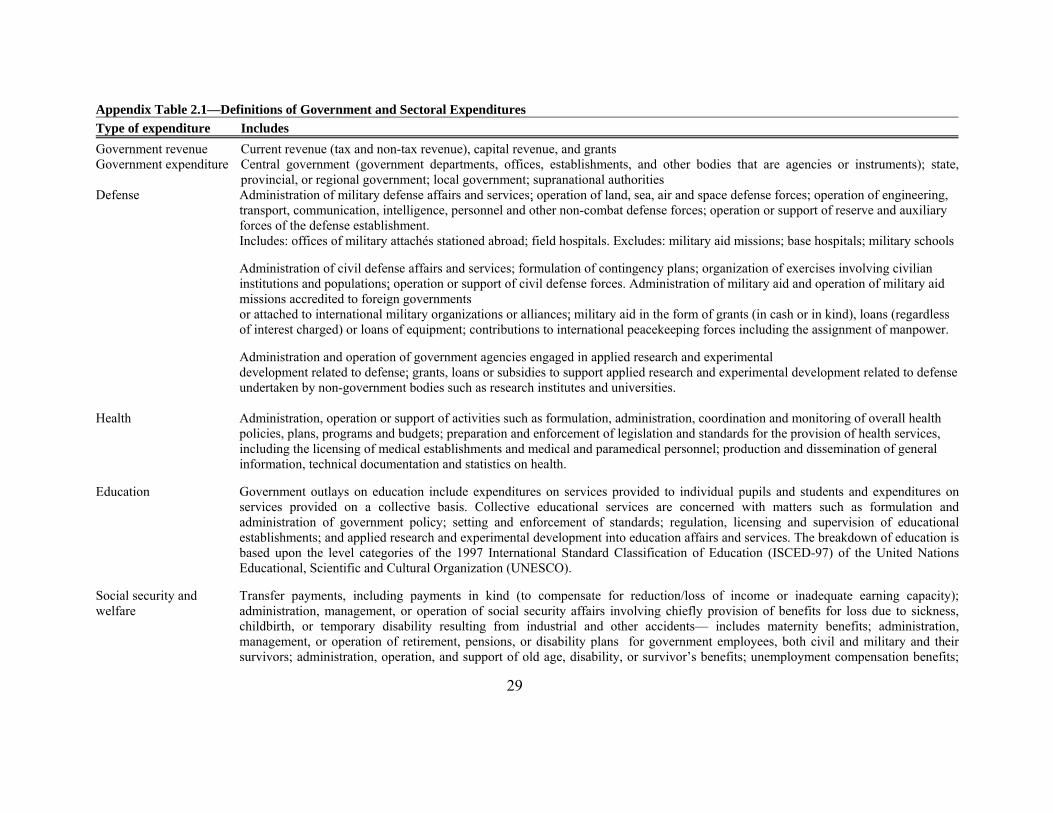
Appendix Table 2.1—Definitions of Government and Sectoral Expenditures Type of expenditure Includes Government revenue Current revenue (tax and non-tax revenue), capital revenue, and grants Government expenditure Central government (government departments, offices, establishments, and other bodies that are agencies or instruments); state,

provincial, or regional government; local government; supranational authorities Defense Administration of military defense affairs and services; operation of land, sea, air and space defense forces; operation of engineering,

transport, communication, intelligence, personnel and other non-combat defense forces; operation or support of reserve and auxiliary forces of the defense establishment. Includes: offices of military attachés stationed abroad; field hospitals. Excludes: military aid missions; base hospitals; military schools Administration of civil defense affairs and services; formulation of contingency plans; organization of exercises involving civilian institutions and populations; operation or support of civil defense forces. Administration of military aid and operation of military aid missions accredited to foreign governments or attached to international military organizations or alliances; military aid in the form of grants (in cash or in kind), loans (regardless of interest charged) or loans of equipment; contributions to international peacekeeping forces including the assignment of manpower. Administration and operation of government agencies engaged in applied research and experimental development related to defense; grants, loans or subsidies to support applied research and experimental development related to defense undertaken by non-government bodies such as research institutes and universities.

Health Administration, operation or support of activities such as formulation, administration, coordination and monitoring of overall health policies, plans, programs and budgets; preparation and enforcement of legislation and standards for the provision of health services, including the licensing of medical establishments and medical and paramedical personnel; production and dissemination of general information, technical documentation and statistics on health.

Education Government outlays on education include expenditures on services provided to individual pupils and students and expenditures on services provided on a collective basis. Collective educational services are concerned with matters such as formulation andadministration of government policy; setting and enforcement of standards; regulation, licensing and supervision of educationalestablishments; and applied research and experimental development into education affairs and services. The breakdown of education isbased upon the level categories of the 1997 International Standard Classification of Education (ISCED-97) of the United Nations Educational, Scientific and Cultural Organization (UNESCO).

Social security and welfare

Transfer payments, including payments in kind (to compensate for reduction/loss of income or inadequate earning capacity); administration, management, or operation of social security affairs involving chiefly provision of benefits for loss due to sickness,childbirth, or temporary disability resulting from industrial and other accidents— includes maternity benefits; administration, management, or operation of retirement, pensions, or disability plans for government employees, both civil and military and theirsurvivors; administration, operation, and support of old age, disability, or survivor’s benefits; unemployment compensation benefits;

30

family and child allowances; welfare affairs and services (children’s and old age residential institutions, handicapped persons, andother residential institutions)

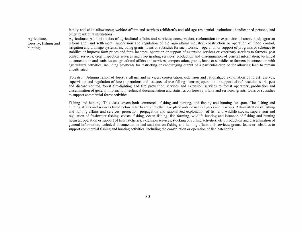
Agriculture, forestry, fishing and hunting

Agriculture: Administration of agricultural affairs and services; conservation, reclamation or expansion of arable land; agrarian reform and land settlement; supervision and regulation of the agricultural industry; construction or operation of flood control, irrigation and drainage systems, including grants, loans or subsidies for such works; �operation or support of programs or schemes to stabilize or improve farm prices and farm incomes; operation or support of extension services or veterinary services to farmers, pestcontrol services, crop inspection services and crop grading services; production and dissemination of general information, technicaldocumentation and statistics on agricultural affairs and services; compensation, grants, loans or subsidies to farmers in connection withagricultural activities, including payments for restricting or encouraging output of a particular crop or for allowing land to remainuncultivated. Forestry: Administration of forestry affairs and services; conservation, extension and rationalized exploitation of forest reserves;supervision and regulation of forest operations and issuance of tree-felling licenses; operation or support of reforestation work, pest and disease control, forest fire-fighting and fire prevention services and extension services to forest operators; production and dissemination of general information, technical documentation and statistics on forestry affairs and services; grants, loans or subsidies to support commercial forest activities Fishing and hunting: This class covers both commercial fishing and hunting, and fishing and hunting for sport. The fishing andhunting affairs and services listed below refer to activities that take place outside natural parks and reserves. Administration of fishing and hunting affairs and services; protection, propagation and rationalized exploitation of fish and wildlife stocks; supervision andregulation of freshwater fishing, coastal fishing, ocean fishing, fish farming, wildlife hunting and issuance of fishing and huntinglicenses; operation or support of fish hatcheries, extension services, stocking or culling activities, etc.; production and dissemination ofgeneral information, technical documentation and statistics on fishing and hunting affairs and services; grants, loans or subsidies tosupport commercial fishing and hunting activities, including the construction or operation of fish hatcheries.

31

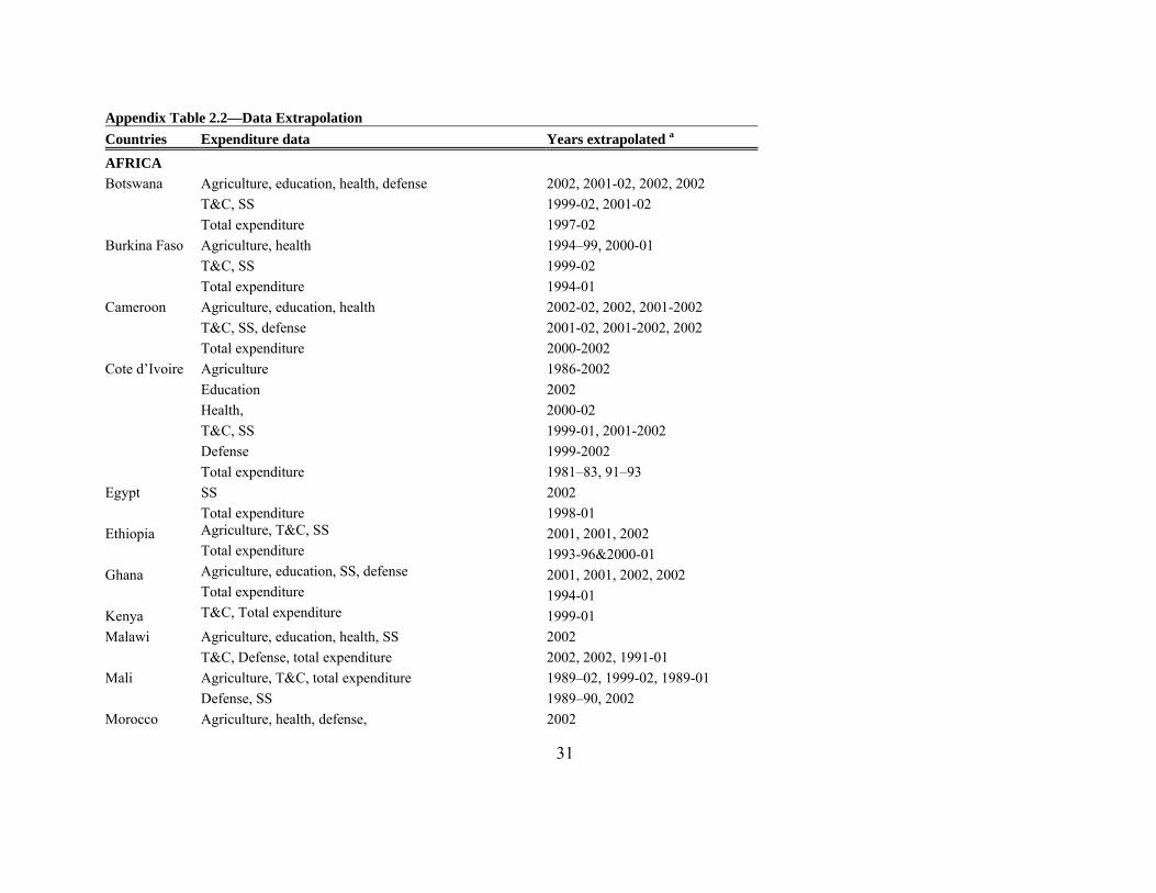
Appendix Table 2.2—Data Extrapolation Countries Expenditure data Years extrapolated a AFRICA Botswana Agriculture, education, health, defense 2002, 2001-02, 2002, 2002 T&C, SS 1999-02, 2001-02 Total expenditure 1997-02 Burkina Faso Agriculture, health 1994–99, 2000-01 T&C, SS 1999-02 Total expenditure 1994-01 Cameroon Agriculture, education, health 2002-02, 2002, 2001-2002 T&C, SS, defense 2001-02, 2001-2002, 2002 Total expenditure 2000-2002 Cote d’Ivoire Agriculture 1986-2002 Education 2002 Health, 2000-02 T&C, SS 1999-01, 2001-2002 Defense 1999-2002 Total expenditure 1981–83, 91–93 Egypt SS 2002 Total expenditure 1998-01 Ethiopia Agriculture, T&C, SS 2001, 2001, 2002 Total expenditure 1993-96&2000-01 Ghana Agriculture, education, SS, defense 2001, 2001, 2002, 2002 Total expenditure 1994-01 Kenya T&C, Total expenditure 1999-01 Malawi Agriculture, education, health, SS 2002 T&C, Defense, total expenditure 2002, 2002, 1991-01 Mali Agriculture, T&C, total expenditure 1989–02, 1999-02, 1989-01 Defense, SS 1989–90, 2002 Morocco Agriculture, health, defense, 2002

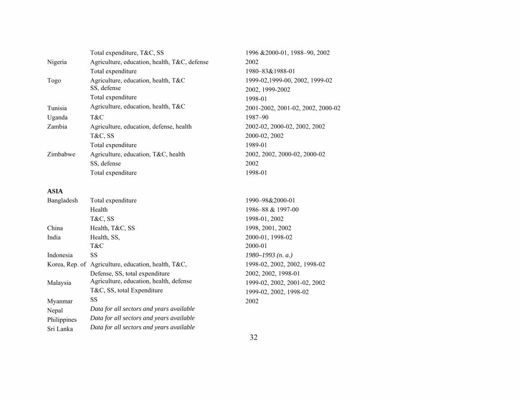
32

Total expenditure, T&C, SS 1996 &2000-01, 1988–90, 2002 Nigeria Agriculture, education, health, T&C, defense 2002 Total expenditure 1980–83&1988-01 Togo Agriculture, education, health, T&C 1999-02,1999-00, 2002, 1999-02 SS, defense 2002, 1999-2002 Total expenditure 1998-01 Tunisia Agriculture, education, health, T&C 2001-2002, 2001-02, 2002, 2000-02Uganda T&C 1987–90 Zambia Agriculture, education, defense, health 2002-02, 2000-02, 2002, 2002 T&C, SS 2000-02, 2002 Total expenditure 1989-01 Zimbabwe Agriculture, education, T&C, health 2002, 2002, 2000-02, 2000-02 SS, defense 2002 Total expenditure 1998-01 ASIA Bangladesh Total expenditure 1990–98&2000-01 Health 1986–88 & 1997-00 T&C, SS 1998-01, 2002 China Health, T&C, SS 1998, 2001, 2002 India Health, SS, 2000-01, 1998-02 T&C 2000-01 Indonesia SS 1980–1993 (n. a.) Korea, Rep. of Agriculture, education, health, T&C, 1998-02, 2002, 2002, 1998-02 Defense, SS, total expenditure 2002, 2002, 1998-01 Malaysia Agriculture, education, health, defense 1999-02, 2002, 2001-02, 2002 T&C, SS, total Expenditure 1999-02, 2002, 1998-02 Myanmar SS 2002 Nepal Data for all sectors and years available Philippines Data for all sectors and years available Sri Lanka Data for all sectors and years available

33

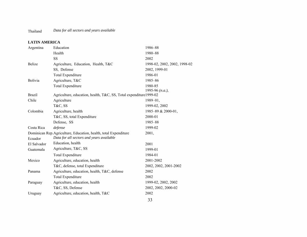
Thailand Data for all sectors and years available LATIN AMERICA Argentina Education 1986–88 Health 1980–88 SS 2002 Belize Agriculture, Education, Health, T&C 1998-02, 2002, 2002, 1998-02 SS, Defense 2002, 1999-01 Total Expenditure 1986-01 Bolivia Agriculture, T&C 1985–86 Total Expenditure 1980-85

Brazil Agriculture, education, health, T&C, SS, Total expenditure1995-96 (n.a.), 1999-02

Chile Agriculture 1989–01, T&C, SS 1999-02, 2002 Colombia Agriculture, health 1985–89 & 2000-01, T&C, SS, total Expenditure 2000-01 Defense, SS 1985–88 Costa Rica defense 1999-02 Dominican Rep.Agriculture, Education, health, total Expenditure 2001, Ecuador Data for all sectors and years available El Salvador Education, health 2001 Guatemala Agriculture, T&C, SS 1999-01 Total Expenditure 1984-01 Mexico Agriculture, education, health 2001-2002 T&C, defense, total Expenditure 2002, 2002, 2001-2002 Panama Agriculture, education, health, T&C, defense 2002 Total Expenditure 2002 Paraguay Agriculture, education, health 1999-02, 2002, 2002 T&C, SS, Defense 2002, 2002, 2000-02 Uruguay Agriculture, education, health, T&C 2002

34

Defense 2000-02 Venezuela Education 1995–98

35

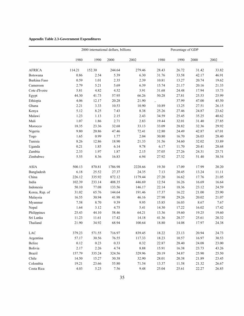
Appendix Table 2.3-Government Expenditures 2000 international dollars, billions Percentage of GDP 1980 1990 2000 2002 1980 1990 2000 2002 AFRICA 114.21 152.30 244.64 279.46 28.43 26.72 31.42 33.82Botswana 0.86 2.54 5.39 6.30 31.76 33.58 42.17 46.91Burkina Faso 0.59 1.01 2.35 2.39 10.81 13.27 20.74 19.62Cameroon 2.79 5.21 5.69 6.39 15.74 21.17 20.16 21.33Cote d'Ivoire 5.81 4.82 4.52 3.91 31.68 24.48 17.94 15.73Egypt 44.30 41.73 57.95 66.26 50.28 27.81 25.53 25.99Ethiopia 4.06 12.17 20.28 21.90 .. 37.99 47.00 45.50Ghana 2.21 3.33 10.53 10.90 10.89 13.25 27.51 26.15Kenya 5.12 8.25 7.43 8.38 25.26 27.46 24.87 23.62Malawi 1.23 1.13 2.15 2.43 34.59 25.45 35.25 40.62Mali 1.07 1.86 2.71 2.83 19.44 32.01 31.40 27.85Morocco 18.35 23.36 32.68 33.13 33.09 28.82 32.36 29.92Nigeria 9.80 20.86 47.46 72.41 12.80 24.49 42.87 67.01Togo 1.65 0.99 1.77 2.04 30.80 16.70 26.03 28.40Tunisia 8.26 12.86 18.90 21.33 31.56 34.60 32.02 33.89Uganda 0.21 1.85 6.14 9.78 6.17 11.70 20.41 28.68Zambia 2.33 1.97 1.87 2.15 37.05 27.26 24.31 25.71Zimbabwe 5.55 8.36 16.83 6.94 27.92 27.32 51.40 38.54 ASIA 500.13 870.81 1786.98 2228.66 19.30 17.09 17.99 20.20Bangladesh 6.18 25.52 27.37 24.35 7.13 20.45 13.24 11.11China 226.12 335.92 872.12 1179.44 27.20 16.62 17.76 21.05India 102.39 233.14 408.35 446.69 12.54 16.26 16.69 16.64Indonesia 50.10 77.08 133.56 146.17 22.14 18.36 23.12 24.59Korea, Rep. of 31.02 65.76 144.64 191.46 17.37 16.22 21.00 25.90Malaysia 16.55 30.94 41.98 46.16 27.98 29.26 20.02 21.07Myanmar 7.58 8.70 9.39 9.95 15.85 16.03 8.67 7.67Nepal 1.64 3.12 4.75 5.41 14.30 17.22 16.02 17.42Philippines 25.43 44.10 58.46 64.21 13.36 19.60 19.25 19.60Sri Lanka 11.23 11.61 17.42 14.18 41.36 28.37 25.61 20.32Thailand 21.90 34.92 68.94 100.64 18.80 14.08 17.97 24.38 LAC 379.23 571.55 716.97 839.45 18.22 23.13 20.94 24.73Argentina 57.17 30.56 76.55 117.33 18.23 10.57 16.97 30.53Belize 0.12 0.23 0.33 0.32 22.87 28.40 24.08 23.00Bolivia 2.17 2.26 4.74 8.88 15.91 16.38 23.73 43.26Brazil 157.79 335.24 324.56 329.96 20.19 34.87 25.90 25.50Chile 14.50 15.27 30.38 32.90 28.01 20.38 21.89 23.45Colombia 19.21 23.66 55.80 71.54 13.37 11.58 21.32 26.67Costa Rica 4.03 5.23 7.56 9.48 25.04 25.61 22.27 26.85

36

Dominican Rep. 3.92 3.48 8.48 9.89 16.92 11.66 16.02 17.27Ecuador 4.05 5.29 8.54 8.96 14.02 14.97 20.20 19.50El Salvador 0.95 1.76 4.96 0.76 17.14 10.90 17.01 2.51Guatemala 3.94 3.01 5.46 5.75 14.32 10.04 12.17 12.25Mexico 82.18 111.90 140.27 192.07 15.75 17.88 15.95 22.07Panama 2.91 2.59 4.31 4.85 30.53 23.70 23.49 26.35Paraguay 1.54 1.93 4.83 4.71 9.85 9.40 19.38 19.15Uruguay 4.80 5.12 9.30 8.21 21.84 23.35 31.47 32.20Venezuela 19.95 24.02 30.90 33.86 18.74 20.73 21.66 25.67 TOTAL 993.57 1594.65 2748.59 3347.57 19.58 19.60 19.44 21.95 Source: Calculated using data from International Monetary Fund's (IMF) Government Financial Statistics Yearbook (various issues).

37

Table 2.4-Agriculture Expenditure

2000 international dollars, billions Percentage of agricultural GDP Ag exp as a % of total exp 1980 1990 2000 2002 1980 1990 2000 2002 1980 1990 2000 2002 AFRICA 7.33 7.85 9.90 12.62 7.40 5.44 5.71 6.72 6.42 5.15 4.05 4.52 Botswana 0.08 0.16 0.23 0.24 24.28 47.99 71.71 73.22 9.71 6.47 4.29 3.89 Burkina Faso 0.03 0.06 0.17 0.41 2.08 2.79 4.38 10.63 5.47 5.83 7.15 17.23 Cameroon 0.06 0.21 0.11 0.10 1.22 3.58 0.95 0.79 2.22 4.06 2.01 1.64 Cote d'Ivoire 0.20 0.14 0.07 0.06 4.17 2.24 1.08 0.99 3.40 2.97 1.46 1.51 Egypt 1.93 1.97 3.97 4.30 12.56 7.13 11.21 11.21 4.35 4.73 6.85 6.50 Ethiopia 0.34 0.60 1.33 1.02 1.49 4.05 6.59 5.50 8.38 4.91 6.55 4.65 Ghana 0.27 0.14 0.27 0.11 2.30 1.21 2.00 0.74 12.23 4.10 2.57 1.02 Kenya 0.43 0.50 0.36 0.38 7.65 6.64 7.05 4.02 8.42 6.03 4.82 4.58 Malawi 0.13 0.13 0.09 0.13 8.97 7.34 4.53 5.85 10.17 11.10 4.30 5.16 Mali 0.09 0.04 0.13 0.26 3.70 1.69 3.93 8.08 8.31 2.33 4.84 9.11 Morocco 1.18 1.16 1.08 1.31 11.59 8.11 7.87 7.35 6.46 4.98 3.29 3.96 Nigeria 0.27 0.61 0.35 2.38 1.80 2.20 1.14 6.79 2.80 2.91 0.74 3.28 Togo 0.12 0.03 0.03 0.04 7.87 1.74 1.23 1.39 7.03 3.51 1.78 1.99 Tunisia 1.20 1.03 1.09 1.18 32.42 17.61 15.02 18.23 14.52 8.00 5.76 5.55 Uganda 0.07 0.07 0.25 0.41 2.80 0.86 2.38 4.18 32.55 3.91 4.00 4.17 Zambia 0.54 0.06 0.10 0.13 60.85 4.36 6.21 7.65 22.97 2.91 5.08 5.94 Zimbabwe 0.39 0.94 0.29 0.15 13.01 20.60 5.36 3.86 7.03 11.18 1.70 2.21 ASIA 74.00 106.54 162.84 191.76 9.44 8.51 9.54 10.57 14.80 12.23 9.11 8.60 Bangladesh 0.80 1.65 3.35 0.77 1.93 4.49 6.59 1.60 13.02 6.46 12.25 3.15 China 27.59 33.54 67.61 84.54 11.03 6.14 8.67 9.73 12.20 9.98 7.75 7.17 India 28.50 48.26 62.03 71.21 9.92 11.98 11.22 12.90 27.84 20.70 15.19 15.94 Indonesia 5.40 6.40 3.03 3.34 9.94 7.47 3.04 3.03 10.77 8.30 2.27 2.29 Korea, Rep. of 1.73 6.23 13.53 17.59 6.55 18.05 41.82 57.56 5.59 9.47 9.36 9.19 Malaysia 1.45 2.08 1.19 1.11 10.83 12.92 6.57 5.52 8.75 6.72 2.85 2.41 Myanmar 1.79 0.81 1.63 1.04 8.02 2.61 2.63 1.45 23.57 9.33 17.38 10.47 Nepal 0.27 0.26 0.27 0.32 4.05 2.99 2.42 2.71 16.39 8.47 5.76 5.91

38

Philippines 1.54 2.99 3.35 3.08 3.22 6.07 7.03 6.33 6.06 6.79 5.73 4.80 Sri Lanka 2.80 0.67 0.75 0.61 40.09 6.87 6.34 4.81 24.99 5.75 4.30 4.30 Thailand 2.12 3.65 6.09 8.15 7.82 11.77 15.49 20.92 9.67 10.45 8.83 8.10 LAC 30.48 11.52 18.16 21.23 19.51 6.79 11.10 11.57 8.04 2.02 2.53 2.53 Argentina 4.49 0.24 0.47 0.78 23.14 1.04 2.24 2.00 7.86 0.80 0.62 0.67 Belize 0.02 0.03 0.02 0.02 12.98 19.96 7.80 8.82 13.61 12.84 5.83 5.49 Bolivia 1.24 0.08 0.24 0.23 51.54 3.98 9.11 8.56 57.29 3.73 5.00 2.60 Brazil 12.62 3.92 9.92 12.32 6.87 4.97 11.39 8.11 8.00 1.17 3.06 3.73 Chile 0.26 0.31 1.17 0.47 6.87 4.97 11.39 8.11 1.77 2.01 3.84 1.42 Colombia 0.08 1.48 0.52 0.58 0.28 4.46 1.60 1.92 0.40 6.25 0.93 0.82 Costa Rica 0.14 0.21 0.22 0.13 4.77 6.66 7.30 4.85 3.39 4.11 2.85 1.40 Dominican Rep. 0.56 0.50 0.64 0.73 11.99 12.55 10.90 10.91 14.28 14.45 7.60 7.35 Ecuador 0.29 0.21 0.29 0.29 2.62 3.45 5.74 3.76 7.26 4.03 3.37 3.20 El Salvador 0.05 0.10 0.16 0.01 2.62 3.45 5.74 3.76 5.80 5.41 3.30 1.46 Guatemala 0.17 0.13 0.14 0.16 2.48 1.64 1.36 1.50 4.30 4.22 2.52 2.75 Mexico 9.54 3.41 3.80 4.77 22.01 7.59 11.64 14.90 11.61 3.05 2.71 2.48 Panama 0.15 0.07 0.07 0.07 18.56 6.29 6.24 5.51 5.29 2.52 1.52 1.47 Paraguay 0.05 0.02 0.27 0.33 1.20 0.44 5.36 5.56 3.47 1.29 5.63 6.96 Uruguay 0.07 0.08 0.11 0.10 2.20 3.79 6.19 4.41 1.36 1.50 1.22 1.27 Venezuela 0.74 0.73 0.13 0.23 14.88 11.78 1.81 4.70 3.71 3.02 0.41 0.69 TOTAL 111.80 125.91 190.89 225.61 10.76 8.04 9.34 10.32 11.25 7.90 6.95 6.74 N. a. means not available. Source: Calculated using data from International Monetary Fund's Government Financial Statistics Yearbook (various issues).

39

Appendix Table 2.5. Unit Root Tests of Key Variables GDP Revenues Expenditures Aid Agricultural Agricultural Expenditures GDP Botswana n n n n n n Burkina Faso y n n n n y Cameroon n n n n n y Cote d'Ivoire n n n n n n Egypt y y n n n y Ethiopia y n n n n y Ghana y y n n n y Kenya y n n n n n Malawi y y n n n n Mali y n n n y y Morocco y y n n n n Nigeria y y n y y n Togo y y n n n n Tunisia y y n n n n Uganda y y n n y n Zambia y y n n n n Zimbabwe n n n n y n Bangladesh y y n n y y China y y y y y y India y y n n n y Indonesia y y y n n n Korea, Rep. y y y n y n Malaysia y y n n y n Myanmar n y y n y n Nepal y n n n y y Philippines y y y n y y Sri Lanka n n y n n n Thailand n n n n n y Argentina y n y n n y Belize y n y n n y Bolivia y n n n n n Brazil y y n n n y Chile y y n n y n Colombia n y y n n n Costa Rica y n n y n n Dominican Rep. y n n n n n

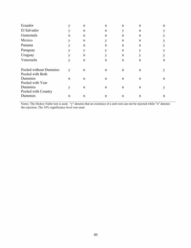
40

Ecuador y n n n n n El Salvador y n n y n y Guatemala n n n n n y Mexico y n y n n y Panama y n n n n y Paraguay y y y n y y Uruguay y n y n y y Venezuela y n n n n n

Pooled without Dummies y n n n n y Pooled with Both Dummies n n n n n n Pooled with Year Dummies y n n n n y Pooled with Country Dummies n n n n n n Notes: The Dickey Fuller test is used. "y" denotes that an existence of a unit root can not be rejected while "n" denotes the rejection. The 10% significance level was used.