1

Cost Minimization and Cost Curves

Beattie, Taylor, and WattsSections: 3.1a, 3.2a-b, 4.1

2

Agenda The Cost Function and General Cost

Minimization Cost Minimization with One Variable

Input Deriving the Average Cost and

Marginal Cost for One Input and One Output

Cost Minimization with Two Variable Inputs

3

Cost Function A cost function is a function that

maps a set of inputs into a cost. In the short-run, the cost function

incorporates both fixed and variable costs.

In the long-run, all costs are considered variable.

4

Cost Function Cont. The cost function can be

represented as the following: C = c(x1, x2, …,xn)= w1*x1 + w2*x2 +

… + wn*xn

Where wi is the price of input i, xi, for i = 1, 2, …, n

Where C is some level of cost and c(•) is a function

5

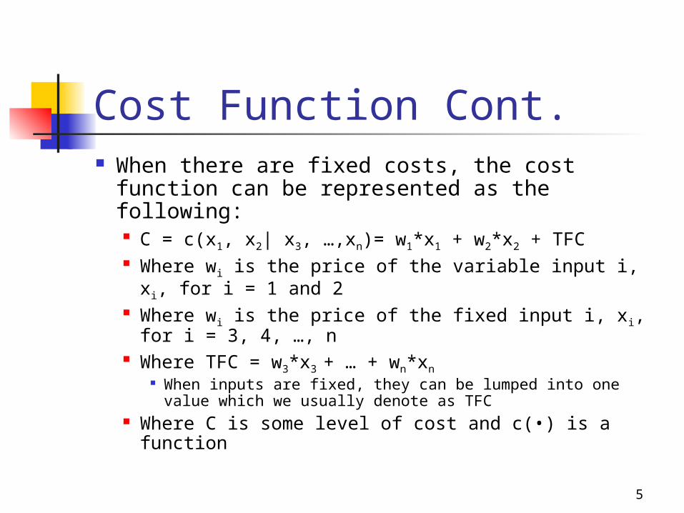
Cost Function Cont. When there are fixed costs, the cost function

can be represented as the following: C = c(x1, x2| x3, …,xn)= w1*x1 + w2*x2 + TFC Where wi is the price of the variable input i, xi, for

i = 1 and 2 Where wi is the price of the fixed input i, xi, for i

= 3, 4, …, n Where TFC = w3*x3 + … + wn*xn

When inputs are fixed, they can be lumped into one value which we usually denote as TFC

Where C is some level of cost and c(•) is a function

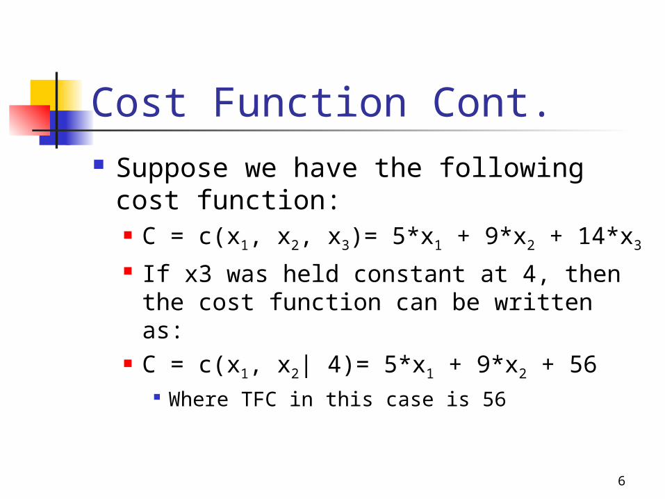
Cost Function Cont. Suppose we have the following

cost function: C = c(x1, x2, x3)= 5*x1 + 9*x2 + 14*x3 If x3 was held constant at 4, then the

cost function can be written as: C = c(x1, x2| 4)= 5*x1 + 9*x2 + 56

Where TFC in this case is 56

6

7

Cost Function Cont. The cost function is usually meaningless

unless you have some constraint that bounds it, i.e., minimum costs occur when all the inputs are equal to zero.

There are two major uses of the cost function: To minimize cost given a certain output

level. To maximize output given a certain cost.

8

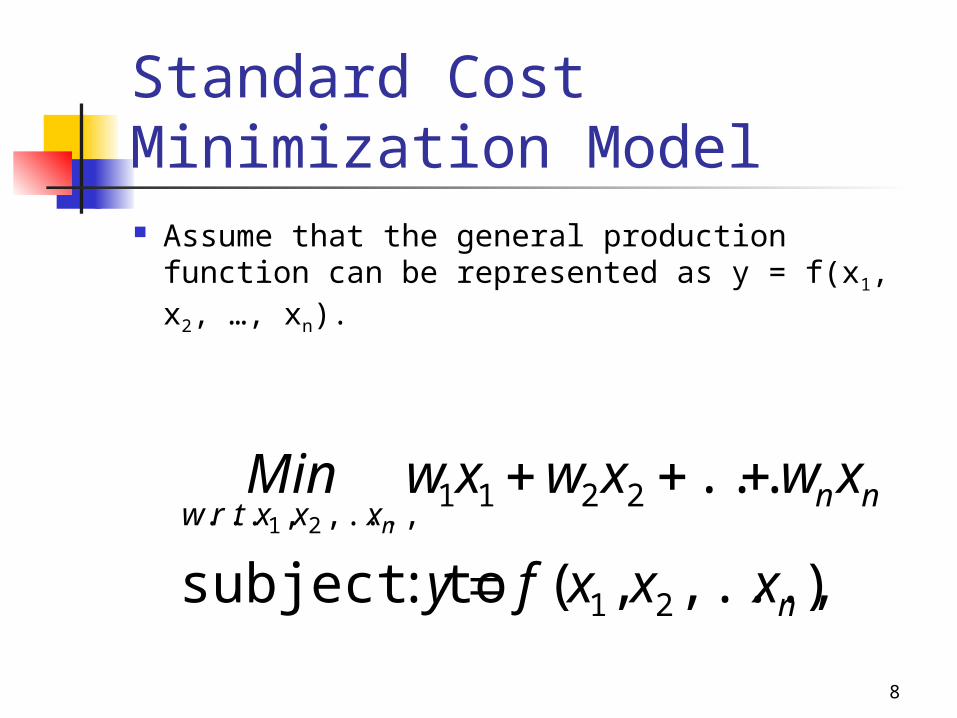
Standard Cost Minimization Model Assume that the general production function

can be represented as y = f(x1, x2, …, xn).

),...,,(:subject to

...

21

2211,...,,... 21

n

nnxxxtrw

xxxfy

xwxwxwMinn

9

Cost Minimization with One Variable Input Assume that we have one variable input (x)

which costs w. Let TFC be the total fixed costs.

Assume that the general production function can be represented as y = f(x).

)(:subject to

...

xfy

TFCwxMinxtrw

10

Cost Minimization with One Variable Input Cont. In the one input, one output world,

the solution to the minimization problem is trivial. By selecting a particular output y, you

are dictating the level of input x. The key is to choose the most

efficient input to obtain the output.

11

Example of Cost Minimization Suppose that you have the following

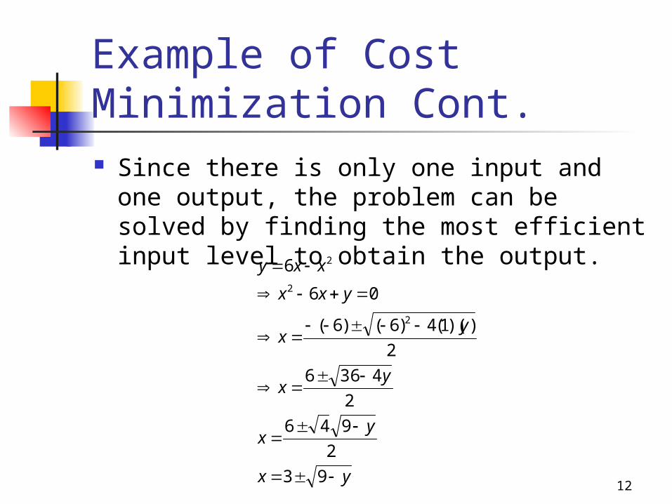
production function: y = f(x) = 6x - x2

You also know that the price of the input is $10 and the total fixed cost is 45.

2

...

6)(:subject to

4510

xxxfy

xMinxtrw

12

Example of Cost Minimization Cont. Since there is only one input and one

output, the problem can be solved by finding the most efficient input level to obtain the output.

yx

yx

yx

yx

yxx

xxy

93

2

946

2

4366

2

))(1(4)6()6(

06

6

2

2

2

13

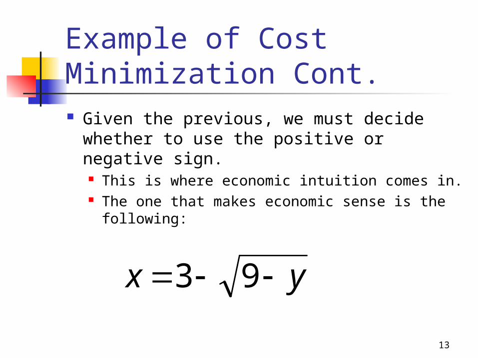
Example of Cost Minimization Cont. Given the previous, we must decide

whether to use the positive or negative sign. This is where economic intuition comes in. The one that makes economic sense is the

following:

yx 93

14

Cost Function and Cost Curves There are many tools that can be

used to understand the cost function: Average Variable Cost (AVC) Average Fixed Cost (AFC) Average Cost (ATC) Marginal Cost (MC)

15

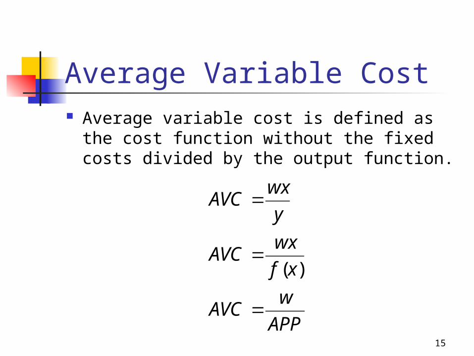
Average Variable Cost Average variable cost is defined as the

cost function without the fixed costs divided by the output function.

APP

wAVC

xf

wxAVC

y

wxAVC

)(

16

Average Fixed Cost Average fixed cost is defined as the cost

function without the variable costs divided by the output function.

)(xf

TFCAFC

y

TFCAFC

17

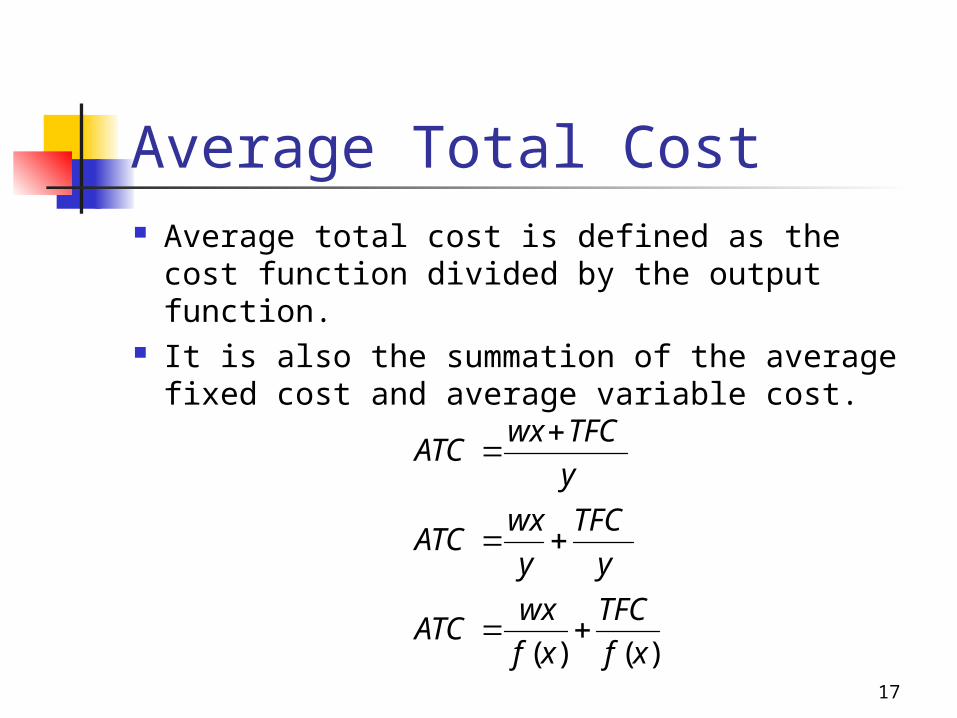
Average Total Cost Average total cost is defined as the cost

function divided by the output function. It is also the summation of the average

fixed cost and average variable cost.

)()( xf

TFC

xf

wxATC

y

TFC

y

wxATC

y

TFCwxATC

18

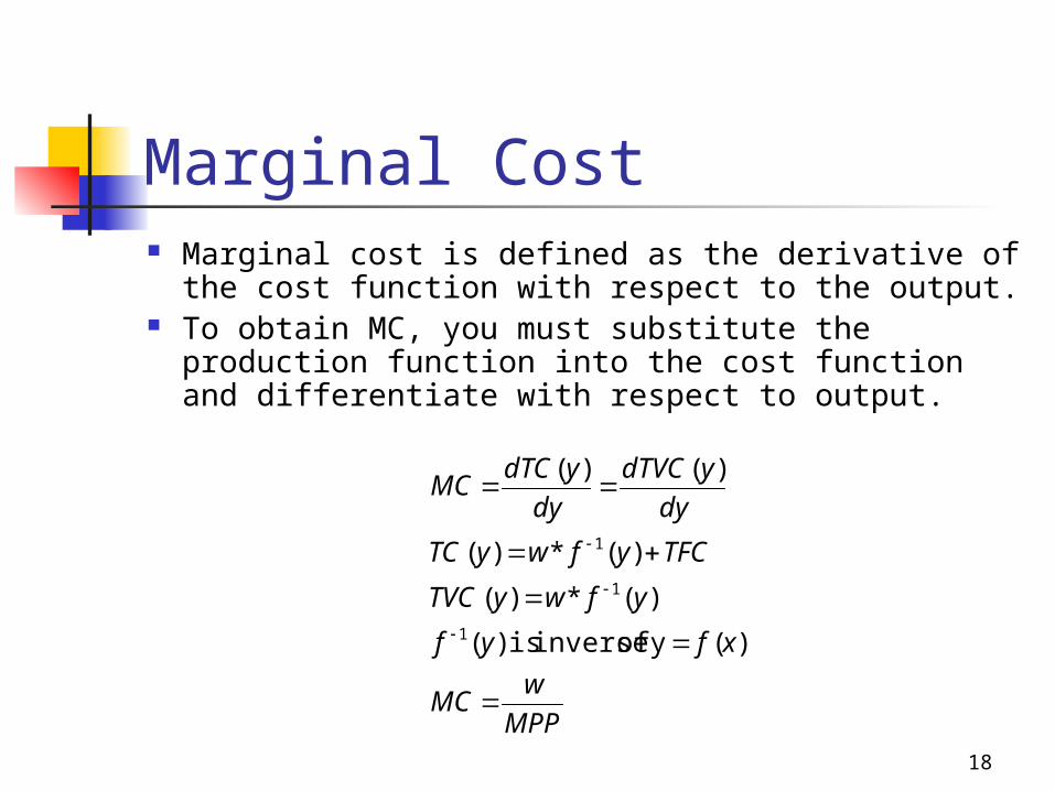
Marginal Cost Marginal cost is defined as the derivative of

the cost function with respect to the output. To obtain MC, you must substitute the

production function into the cost function and differentiate with respect to output.

MPP

wMC

xfyf

yfwyTVC

TFCyfwyTC

dy

ydTVC

dy

ydTCMC

)(y of inverse is )(

)(*)(

)(*)(

)()(

1

1

1

19

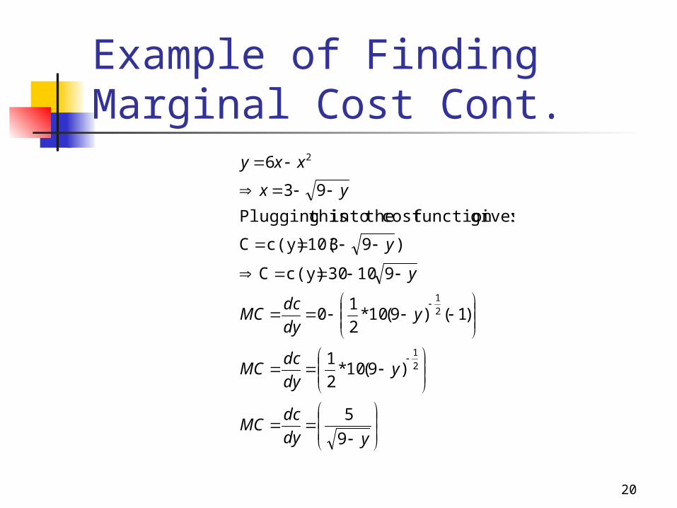
Example of Finding Marginal Cost Using the production function y = f(x)

= 6x - x2, and a price of 10, find the MC by differentiating with respect to y.

To solve this problem, you need to solve the production function for x and plug it into the cost function. This gives you a cost function that is a

function of y.

20

Example of Finding Marginal Cost Cont.

ydy

dcMC

ydy

dcMC

ydy

dcMC

y

y

yx

xxy

9

5

)9(10*2

1

)1()9(10*2

10

91030c(y)C

)9310(c(y)C

:givesfunction cost theinto thisPlugging

93

6

2

1

2

1

2

21

Notes on Costs MC will meet AVC and ATC from

below at the corresponding minimum point of each. Why?

As output increases AFC goes to zero.

As output increases, AVC and ATC get closer to each other.

22

Production and Cost Relationships Summary Cost curves are derived from the

physical production process. The two major relationships

between the cost curves and the production curves: AVC = w/APP MC = w/MPP

23

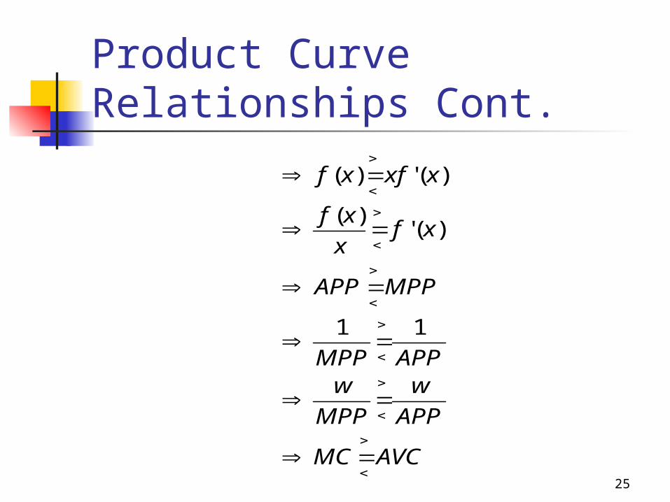
Product Curve Relationships When MPP>APP, APP is increasing.

This implies that when MC<AVC, then AVC is decreasing.

When MPP=APP, APP is at a maximum. This implies that when MC=AVC, then AVC

is at a minimum. When MPP<APP, APP is decreasing.

This implies that when MC>AVC, then AVC is increasing.

24

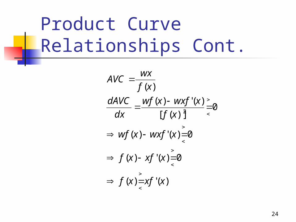
Product Curve Relationships Cont.

)(')(

0)(')(

0)(')(

0)]([

)(')(

)(

2

xxfxf

xxfxf

xwxfxwf

xf

xwxfxwf

dx

dAVC

xf

wxAVC

25

Product Curve Relationships Cont.

AVCMC

APP

w

MPP

wAPPMPP

MPPAPP

xfx

xf

xxfxf

11

)(')(

)(')(

26

Example of Examining the Relationship Between MC and AVC

Given that the production function y = f(x) = 6x - x2, and a price of 10, find the input(s) where AVC is greater than, equal to, and less than MC.

To solve this, examine the following situations: AVC = MC AVC > MC AVC < MC

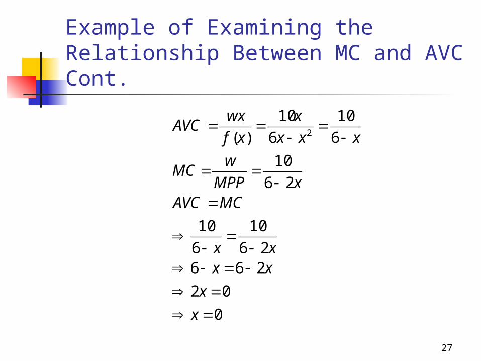
27

Example of Examining the Relationship Between MC and AVC Cont.

0

02

26626

10

6

10

26

10

6

10

6

10

)( 2

x

x

xxxx

MCAVCxMPP

wMC

xxx

x

xf

wxAVC

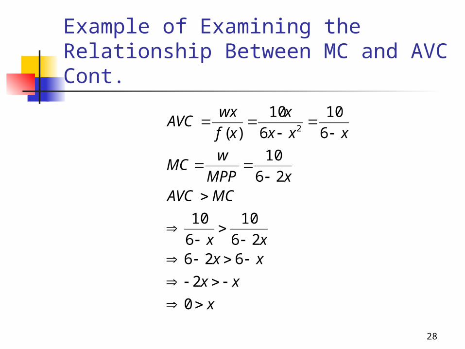
28

Example of Examining the Relationship Between MC and AVC Cont.

x

xx

xxxx

MCAVCxMPP

wMC

xxx

x

xf

wxAVC

0

2

62626

10

6

10

26

10

6

10

6

10

)( 2

29

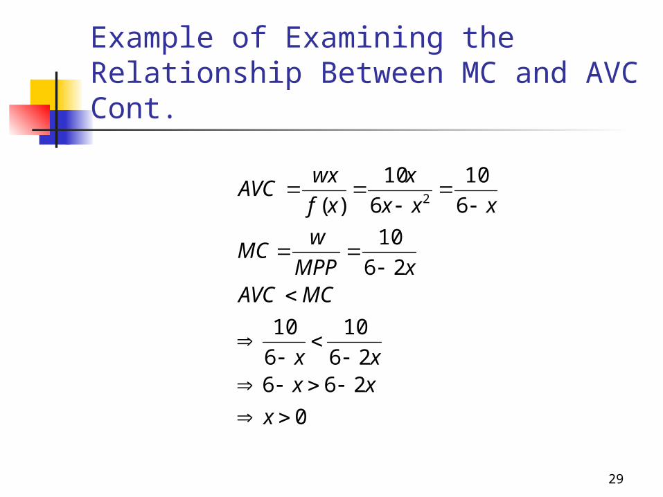
Example of Examining the Relationship Between MC and AVC Cont.

0

26626

10

6

10

26

10

6

10

6

10

)( 2

x

xxxx

MCAVCxMPP

wMC

xxx

x

xf

wxAVC

30

Review of the Iso-Cost Line The iso-cost line is a graphical

representation of the cost function with two inputs where the total cost C is held to some fixed level. C = c(x1,x2)=w1x1 + w2x2

31

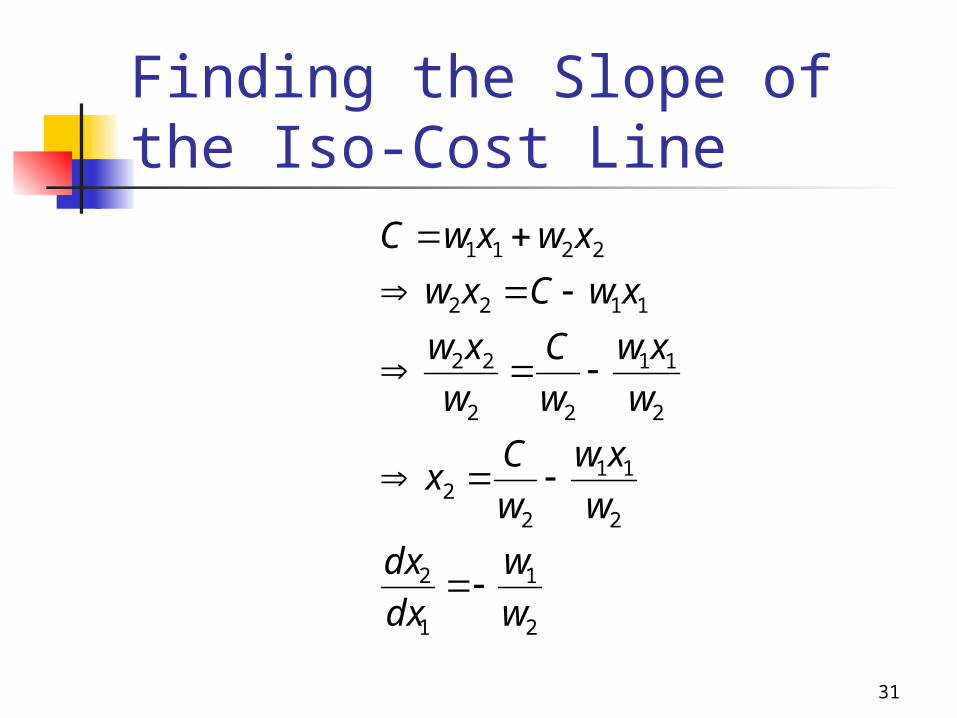
Finding the Slope of the Iso-Cost Line

2

1

1

2

2

11

22

2

11

22

22

1122

2211

w

w

dx

dx

w

xw

w

Cx

w

xw

w

C

w

xw

xwCxw

xwxwC

32

Example of Iso-Cost Line Suppose you had $1000 to spend

on the production of lettuce. To produce lettuce, you need two

inputs labor and machinery. Labor costs you $10 per unit, while

machinery costs $100 per unit.

33

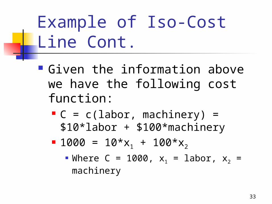
Example of Iso-Cost Line Cont. Given the information above we

have the following cost function: C = c(labor, machinery) = $10*labor

+ $100*machinery 1000 = 10*x1 + 100*x2

Where C = 1000, x1 = labor, x2 = machinery

34

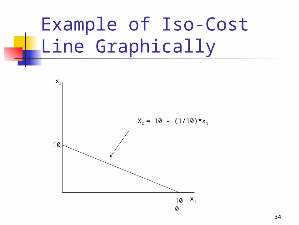
Example of Iso-Cost Line Graphically

x2

x1

10

100

X2 = 10 – (1/10)*x1

35

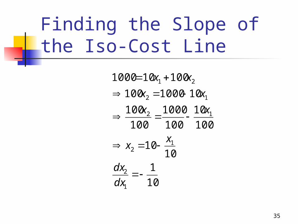
Finding the Slope of the Iso-Cost Line

10

110

10

100

10

100

1000

100

100

101000100

100101000

1

2

12

12

12

21

dx

dx

xx

xx

xx

xx

36

Notes on Iso-Cost Line As you increase C, you shift the

iso-cost line parallel out. As you change one of the costs of

an input, the iso-cost line rotates.

37

Input Use Selection There are two ways of examining how

to select the amount of each input used in production. Maximize output given a certain cost

constraint Minimize cost given a fixed level of

output Both give the same input selection

rule.

38

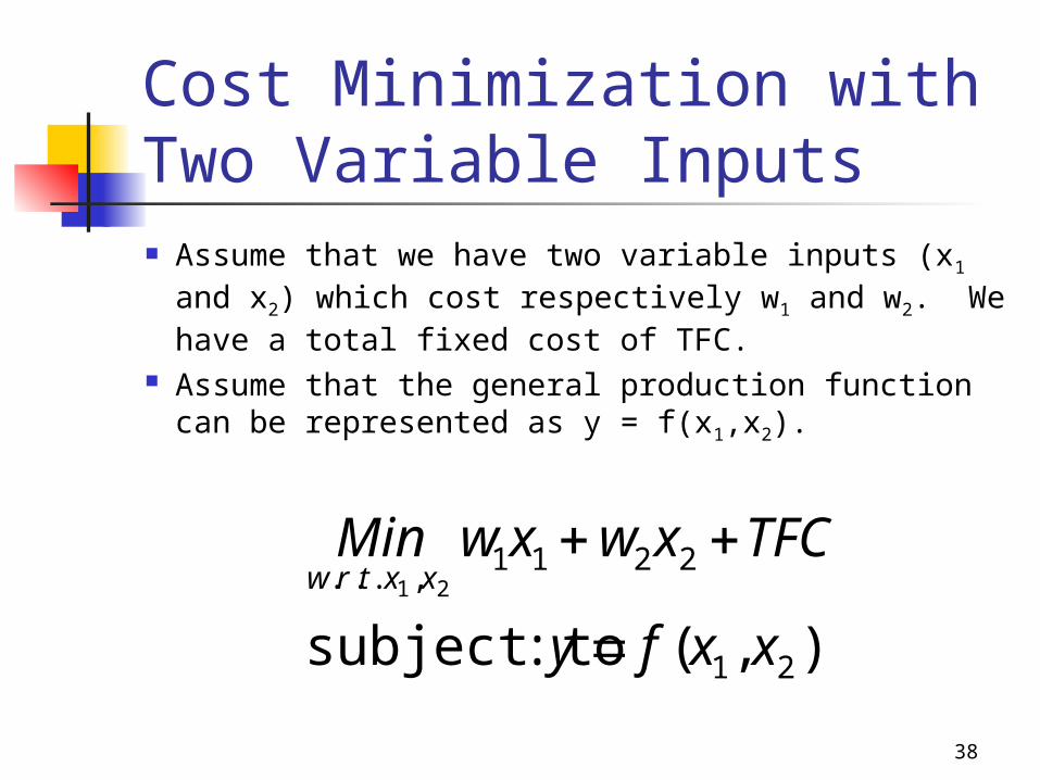
Cost Minimization with Two Variable Inputs Assume that we have two variable inputs (x1 and

x2) which cost respectively w1 and w2. We have a total fixed cost of TFC.

Assume that the general production function can be represented as y = f(x1,x2).

),(:subject to 21

2211,... 21

xxfy

TFCxwxwMinxxtrw

39

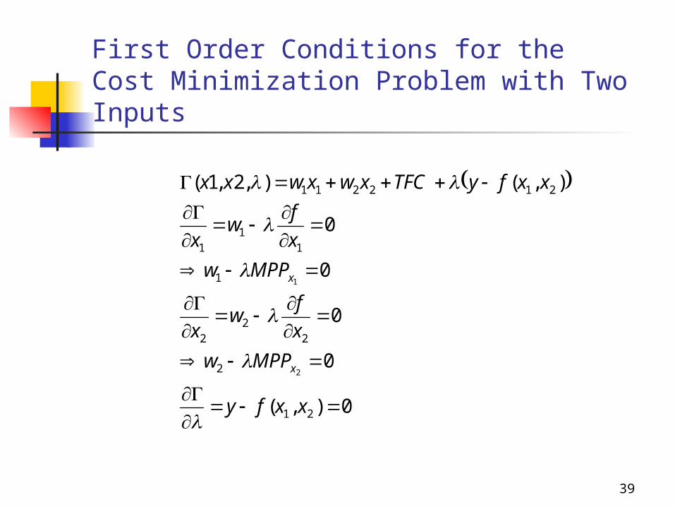
First Order Conditions for the Cost Minimization Problem with Two Inputs

0),(

0

0

0

0

),(),2,1(

21

2

22

2

1

11

1

212211

2

1

xxfy

MPPw

x

fw

x

MPPw

x

fw

x

xxfyTFCxwxwxx

x

x

40

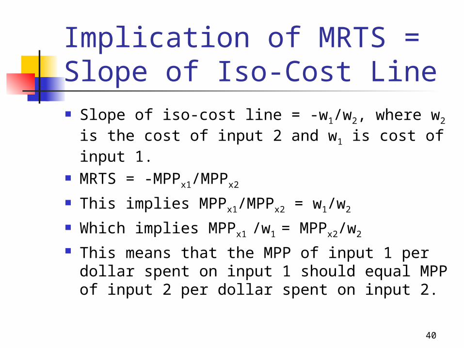
Implication of MRTS = Slope of Iso-Cost Line Slope of iso-cost line = -w1/w2, where w2 is

the cost of input 2 and w1 is cost of input 1. MRTS = -MPPx1/MPPx2 This implies MPPx1/MPPx2 = w1/w2

Which implies MPPx1 /w1 = MPPx2/w2

This means that the MPP of input 1 per dollar spent on input 1 should equal MPP of input 2 per dollar spent on input 2.

41

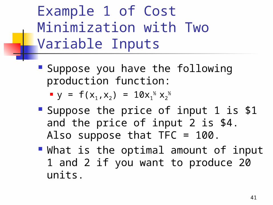
Example 1 of Cost Minimization with Two Variable Inputs

Suppose you have the following production function: y = f(x1,x2) = 10x1

½ x2½

Suppose the price of input 1 is $1 and the price of input 2 is $4. Also suppose that TFC = 100.

What is the optimal amount of input 1 and 2 if you want to produce 20 units.

42

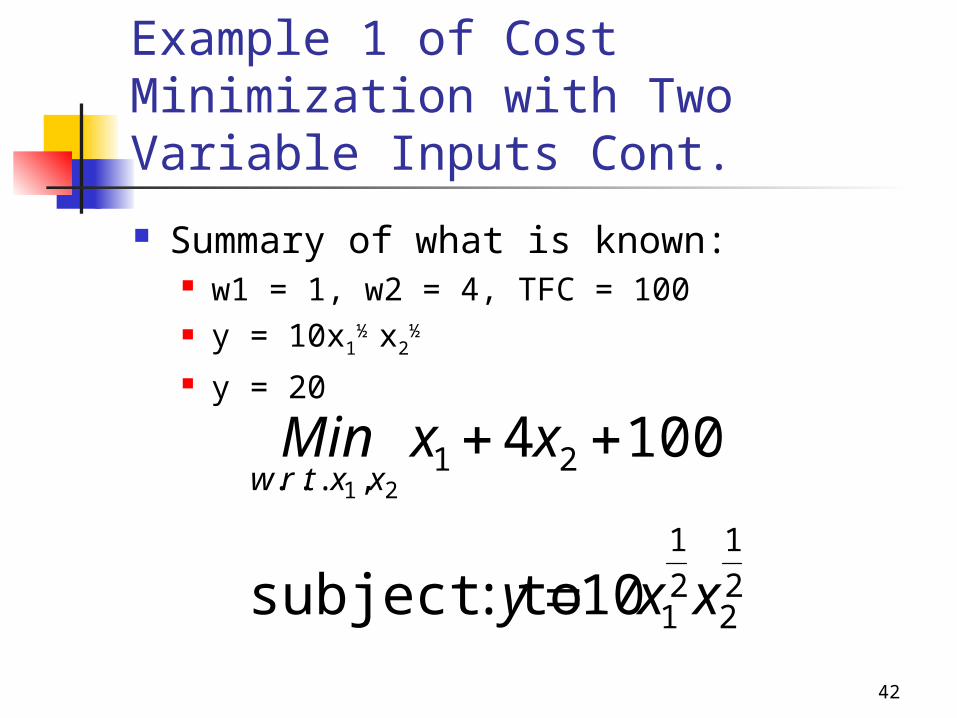
Example 1 of Cost Minimization with Two Variable Inputs Cont.

Summary of what is known: w1 = 1, w2 = 4, TFC = 100 y = 10x1

½ x2½

y = 20

2

1

22

1

1

21,...

10:subject to

100421

xxy

xxMinxxtrw

43

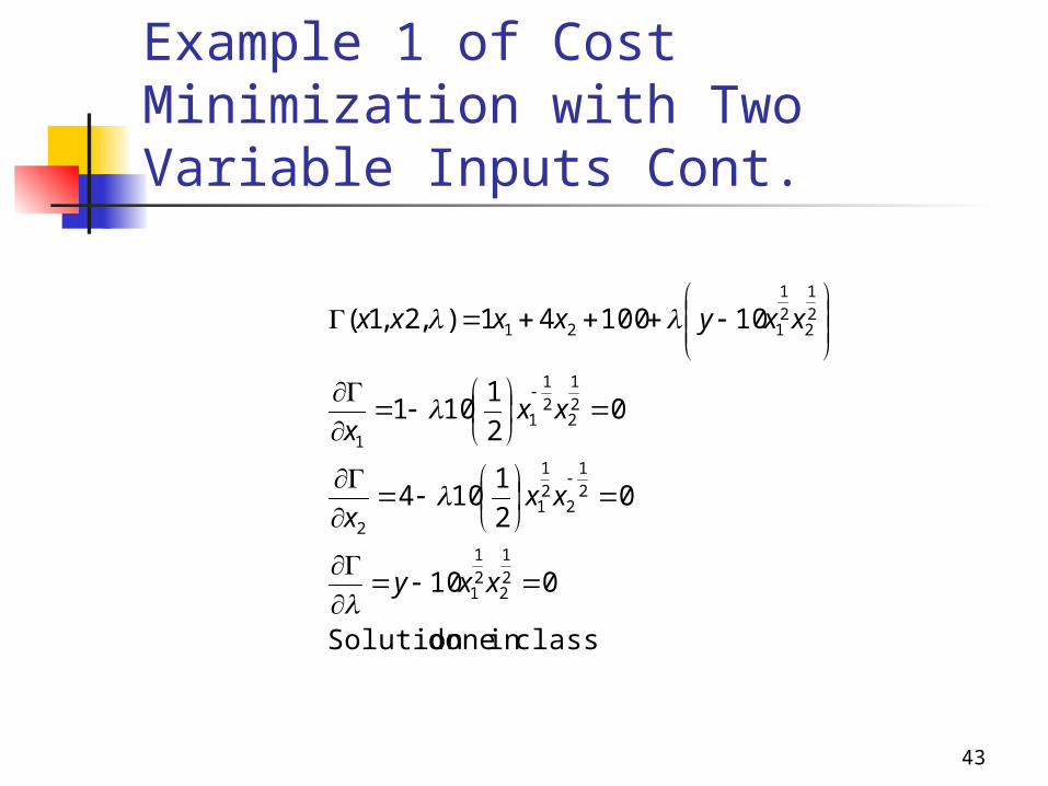
Example 1 of Cost Minimization with Two Variable Inputs Cont.

classin doneSolution

010

02

1104

02

1101

1010041),2,1(

2

1

22

1

1

2

1

22

1

12

2

1

22

1

11

2

1

22

1

121

xxy

xxx

xxx

xxyxxxx

44

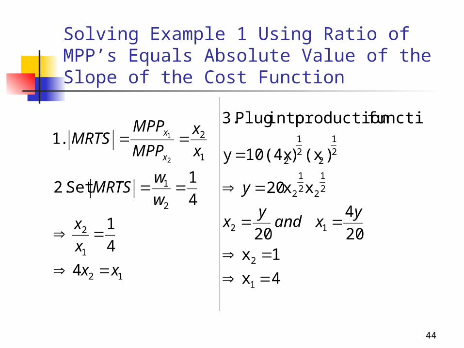
Solving Example 1 Using Ratio of MPP’s Equals Absolute Value of the Slope of the Cost Function

4x

1x20

4

20

xx20

)(x)10(4xy

function production into Plug3.

4

4

1

4

1Set 2.

.1

1

2

12

2

1

22

1

2

2

1

22

1

2

12

1

2

2

1

1

2

2

1

yxand

yx

y

xx

x

x

w

wMRTS

x

x

MPP

MPPMRTS

x

x

45

Solving Example 1 Using MRTS from the Isoquant and Setting it Equal to the Slope of the Cost Function

4x

1x

205100

usingfor x Solve .4520

44

1

100

4

1Set3.

100MRTS

MRTS 2.Find

100100

Isoquant Find .1

1

2

12

2

12

1

21

2

2

1

21

2

1

2

11

2

1

2

2

yyyx

x

yyx

xy

w

wMRTS

xy

x

x

xy

x

yx

46

Final Note on Input Selection It does not matter whether you are

trying to maximize output given a fixed cost level or minimizing a cost given a fixed output level, you want to have the iso-cost line tangent to the isoquant. This implies that you will set the absolute

value of MRTS equal to the absolute value of the slope of the iso-cost line.