1 1 slide ©2009. econ-2030-applied statistics (dr. tadesse) chapter 9 learning objectives...
Post on 19-Dec-2015
221 views
TRANSCRIPT

1 1 Slide
Slide
©2009. Econ-2030-Applied Statistics (Dr. Tadesse)
Chapter 9 Learning Objectives
Population Mean: s Unknown
Population Proportion

2 2 Slide
Slide
©2009. Econ-2030-Applied Statistics (Dr. Tadesse)
Tests About a Population Mean:s Unknown
3 3 Slide
Slide
©2009. Econ-2030-Applied Statistics (Dr. Tadesse)
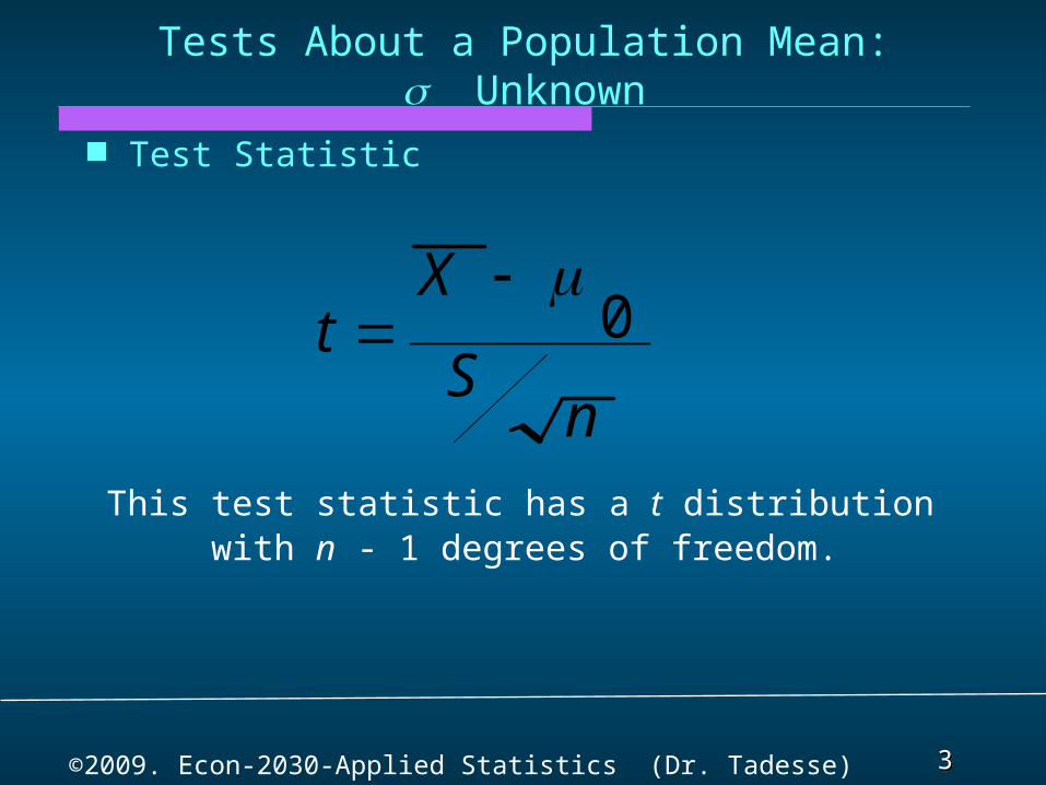
Test Statistic
Tests About a Population Mean:s Unknown
nS
Xt 0
This test statistic has a t distribution with n - 1 degrees of freedom.
4 4 Slide
Slide
©2009. Econ-2030-Applied Statistics (Dr. Tadesse)
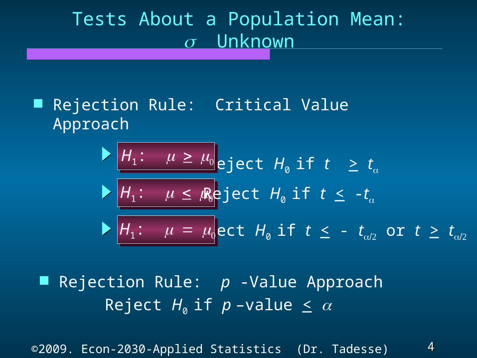
Rejection Rule: p -Value Approach
H1: Reject H0 if t < -t
Reject H0 if t > t
Reject H0 if t < - t or t > t
H1:
H1:
Tests About a Population Mean:s Unknown
Rejection Rule: Critical Value Approach
Reject H0 if p –value < a

5 5 Slide
Slide
©2009. Econ-2030-Applied Statistics (Dr. Tadesse)
p -Values and the t Distribution
The format of the t distribution table provided in most statistics textbooks does not have sufficient detail to determine the exact p-value for a hypothesis test.
However, we can still use the t distribution table to identify a range for the p-value.
An advantage of computer software packages is that the computer output will provide the p-value for the t distribution.
6 6 Slide
Slide
©2009. Econ-2030-Applied Statistics (Dr. Tadesse)
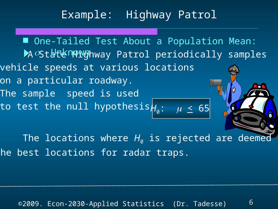
A State Highway Patrol periodically samplesvehicle speeds at various locationson a particular roadway. The sample speed is used to test the null hypothesis
Example: Highway Patrol
One-Tailed Test About a Population Mean: s Unknown
The locations where H0 is rejected are deemed
the best locations for radar traps.
H0: m < 65
7 7 Slide
Slide
©2009. Econ-2030-Applied Statistics (Dr. Tadesse)
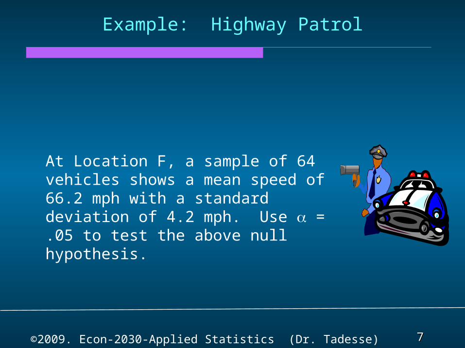
Example: Highway Patrol
At Location F, a sample of 64 vehicles shows a mean speed of 66.2 mph with a standard deviation of 4.2 mph. Use a = .05 to test the above null hypothesis.
8 8 Slide
Slide
©2009. Econ-2030-Applied Statistics (Dr. Tadesse)
One-Tailed Test About a Population Mean:s Unknown
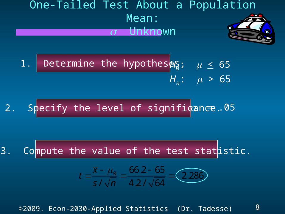
1. Determine the hypotheses.
2. Specify the level of significance.
3. Compute the value of the test statistic.
a = .05
H0: < 65
Ha: m > 65
0 66.2 65
2.286/ 4.2/ 64
xt
s n
9 9 Slide
Slide
©2009. Econ-2030-Applied Statistics (Dr. Tadesse)
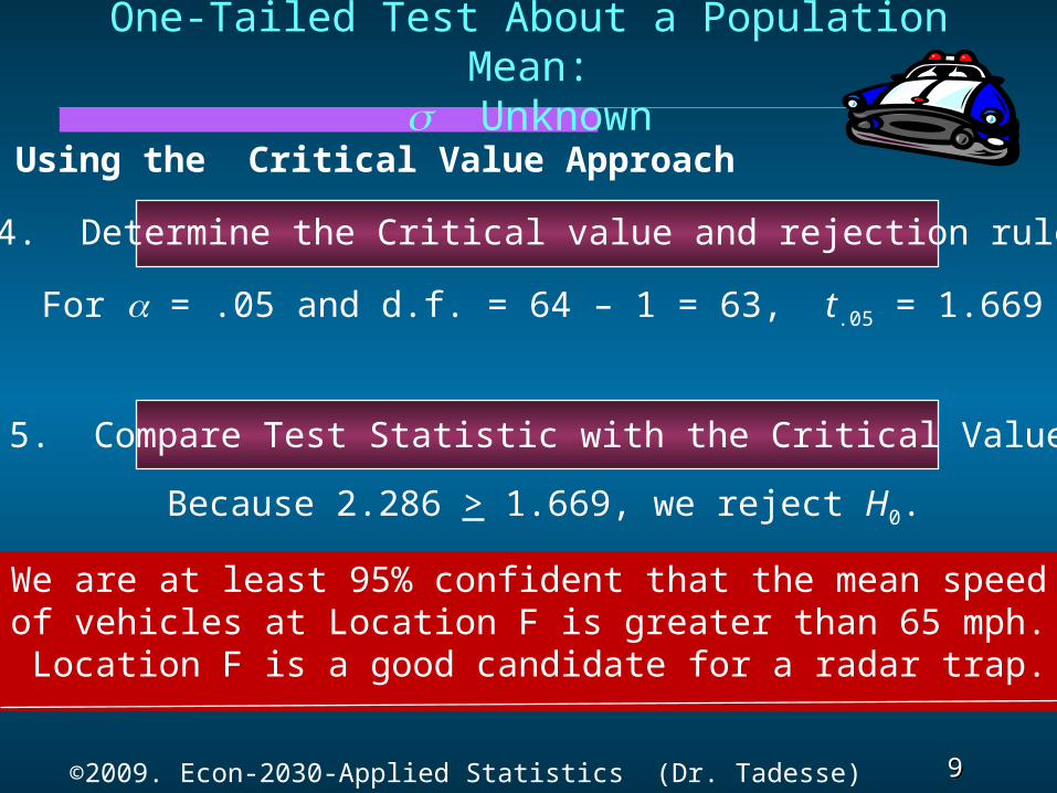
Using the Critical Value Approach
5. Compare Test Statistic with the Critical Value
We are at least 95% confident that the mean speed of vehicles at Location F is greater than 65 mph. Location F is a good candidate for a radar trap.
Because 2.286 > 1.669, we reject H0.
One-Tailed Test About a Population Mean:s Unknown
For a = .05 and d.f. = 64 – 1 = 63, t.05 = 1.669
4. Determine the Critical value and rejection rule.
10 10 Slide
Slide
©2009. Econ-2030-Applied Statistics (Dr. Tadesse)
One-Tailed Test About a Population Mean:s Unknown
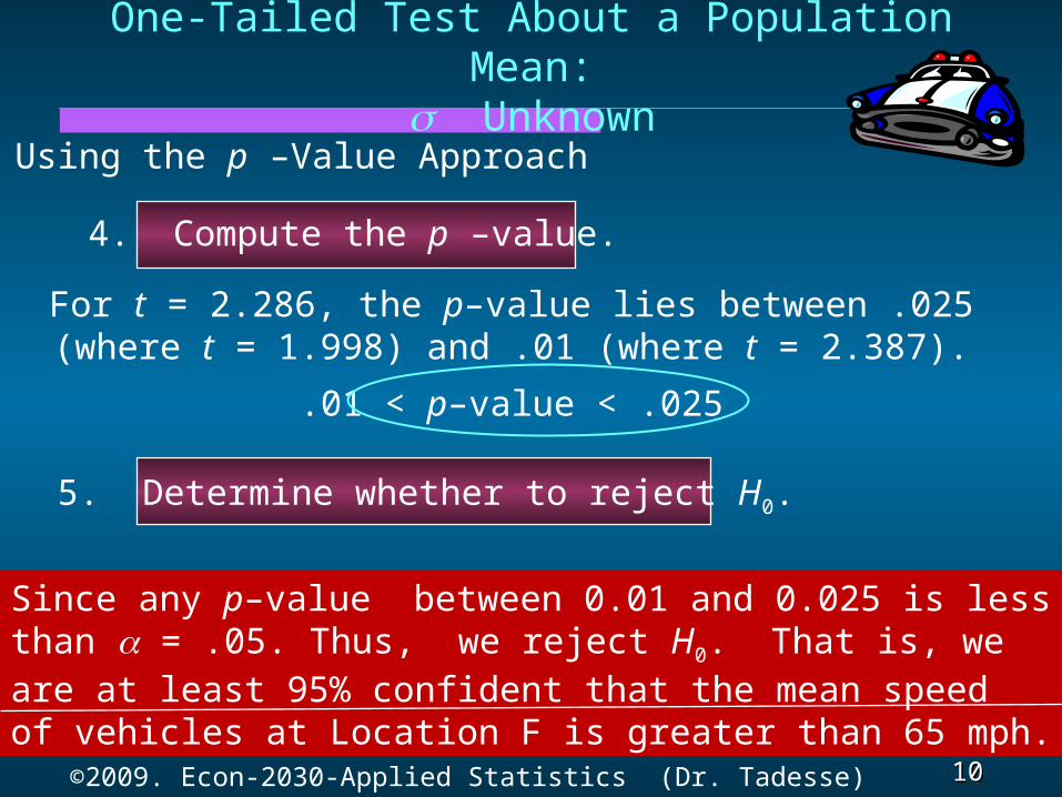
Using the p –Value Approach
5. Determine whether to reject H0.
4. Compute the p –value.
For t = 2.286, the p–value lies between .025(where t = 1.998) and .01 (where t = 2.387).
.01 < p–value < .025
Since any p–value between 0.01 and 0.025 is less than a = .05. Thus, we reject H0. That is, we are at least 95% confident that the mean speed of vehicles at Location F is greater than 65 mph.
12 12 Slide
Slide
©2009. Econ-2030-Applied Statistics (Dr. Tadesse)
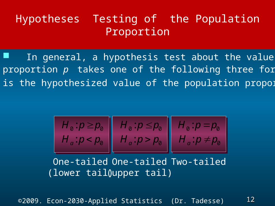
In general, a hypothesis test about the value of a population proportion p takes one of the following three forms (where p0
is the hypothesized value of the population proportion).
Hypotheses Testing of the Population Proportion
One-tailed(lower tail)
One-tailed(upper tail)
Two-tailed
0 0: H p p
0: aH p p0: aH p p0 0: H p p 0 0: H p p
0: aH p p
13 13 Slide
Slide
©2009. Econ-2030-Applied Statistics (Dr. Tadesse)
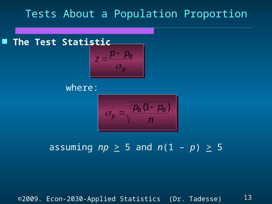
The Test Statistic
zp p
p
0
pp p
n 0 01( )
Tests About a Population Proportion
where:
assuming np > 5 and n(1 – p) > 5

14 14 Slide
Slide
©2009. Econ-2030-Applied Statistics (Dr. Tadesse)
When Using the p –Value Approach
H1 : pp Reject H0 if z > z
Reject H0 if z < -z
Reject H0 if z < -z or z > z
H1: p p
H1 pp
Tests About a Population Proportion
Reject H0 if p –value < a
When using the Critical Value Approach
15 15 Slide
Slide
©2009. Econ-2030-Applied Statistics (Dr. Tadesse)
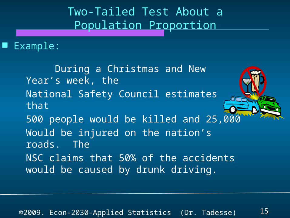
Example:
During a Christmas and New Year’s week, theNational Safety Council estimates that500 people would be killed and 25,000Would be injured on the nation’s roads. TheNSC claims that 50% of the accidents would be caused by drunk driving.
Two-Tailed Test About aPopulation Proportion
16 16 Slide
Slide
©2009. Econ-2030-Applied Statistics (Dr. Tadesse)
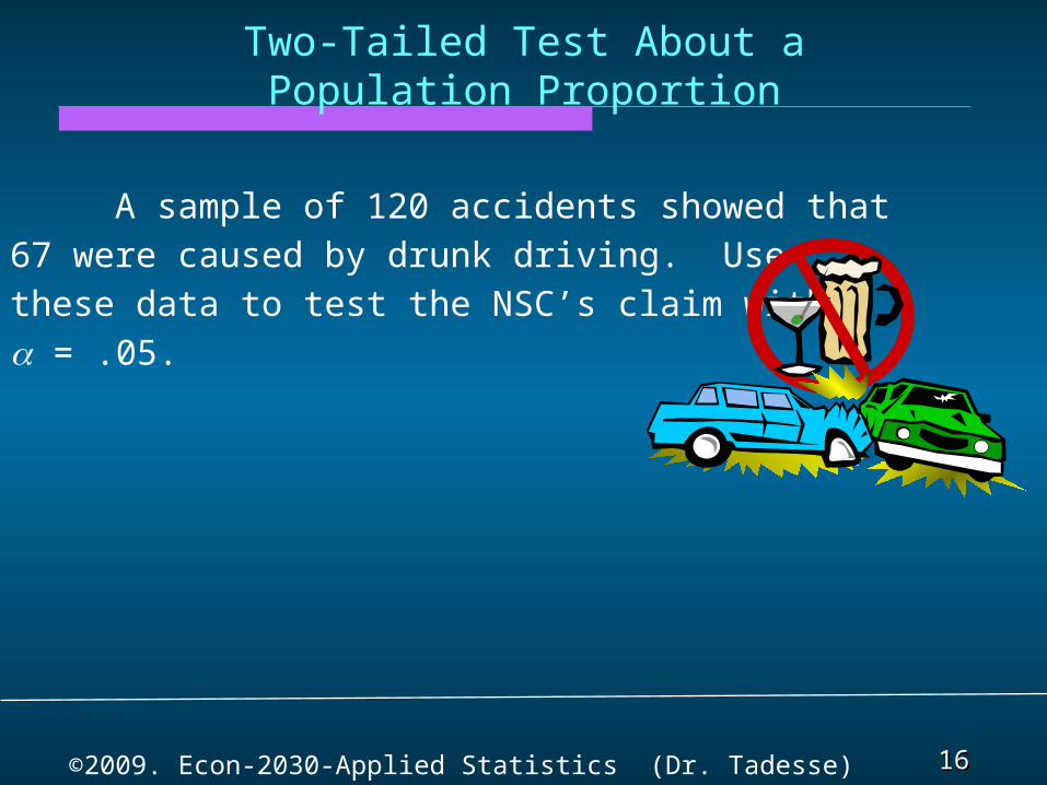
A sample of 120 accidents showed that67 were caused by drunk driving. Usethese data to test the NSC’s claim witha = .05.
Two-Tailed Test About aPopulation Proportion
17 17 Slide
Slide
©2009. Econ-2030-Applied Statistics (Dr. Tadesse)
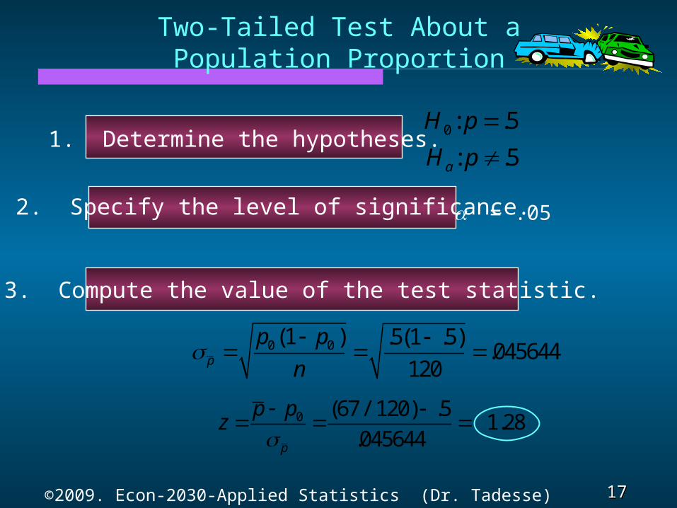
Two-Tailed Test About aPopulation Proportion
1. Determine the hypotheses.
2. Specify the level of significance.
3. Compute the value of the test statistic.
a = .05
0: .5H p
: .5aH p
0 (67/ 120) .5 1.28
.045644p
p pz
0 0(1 ) .5(1 .5).045644
120p
p pn

18 18 Slide
Slide
©2009. Econ-2030-Applied Statistics (Dr. Tadesse)
Two-Tailed Test About aPopulation Proportion
Using the Critical Value Approach
5. Compare the Test Statistic with the Critical Value
For a/2 = .05/2 = .025, z.025 = 1.96. Since the alternative is non-directional, the rejection regionwould be the area below -1.96 and above 1.96
4. Determine the critical value
As 1.278 falls between -1.96 and 1.96 (the acceptance region), we cannot reject H0.
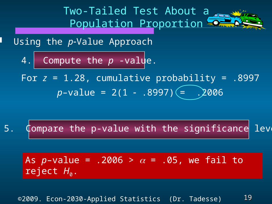
19 19 Slide
Slide
©2009. Econ-2030-Applied Statistics (Dr. Tadesse)
Using the p-Value Approach
4. Compute the p -value.
5. Compare the p-value with the significance level
As p–value = .2006 > a = .05, we fail to reject H0.
Two-Tailed Test About aPopulation Proportion
For z = 1.28, cumulative probability = .8997
p–value = 2(1 - .8997) = .2006