1 1 slide © 2005 thomson/south-western emgt 501 hw solutions problem 13- 10 problem 13 - 21
Post on 19-Dec-2015
215 views
TRANSCRIPT
1 1 Slide
Slide
© 2005 Thomson/South-Western© 2005 Thomson/South-Western
EMGT 501
HW Solutions
Problem 13- 10Problem 13 - 21
2 2 Slide
Slide
© 2005 Thomson/South-Western© 2005 Thomson/South-Western
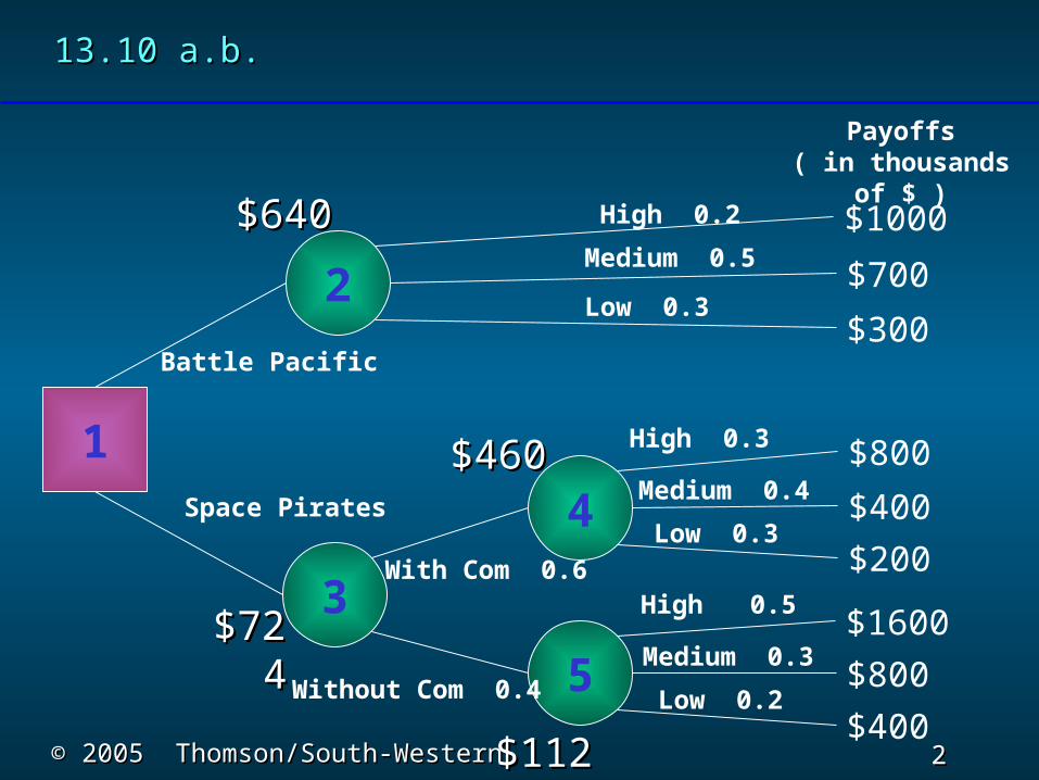
13.10 a.b.13.10 a.b.
1
2
4
5
3
$1000
$700
$300
$800
$400
$200
$1600
$800
$400
Payoffs( in thousands of $ )
High 0.2
Medium 0.5
Low 0.3
Without Com 0.4
With Com 0.6
High 0.3
Medium 0.4
Low 0.3
High 0.5
Medium 0.3
Low 0.2
Battle Pacific
Space Pirates
$640$640
$460$460
$11$112200
$72$7244
3 3 Slide
Slide
© 2005 Thomson/South-Western© 2005 Thomson/South-Western
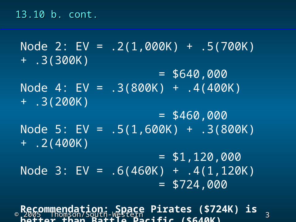
13.10 b. cont.13.10 b. cont.
Node 2: EV = .2(1,000K) + .5(700K) + .3(300K) = $640,000Node 4: EV = .3(800K) + .4(400K) + .3(200K) = $460,000Node 5: EV = .5(1,600K) + .3(800K) + .2(400K) = $1,120,000Node 3: EV = .6(460K) + .4(1,120K) = $724,000
Recommendation: Space Pirates ($724K) is better than Battle Pacific ($640K).
4 4 Slide
Slide
© 2005 Thomson/South-Western© 2005 Thomson/South-Western
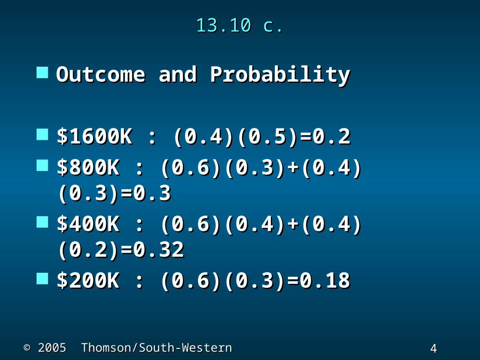
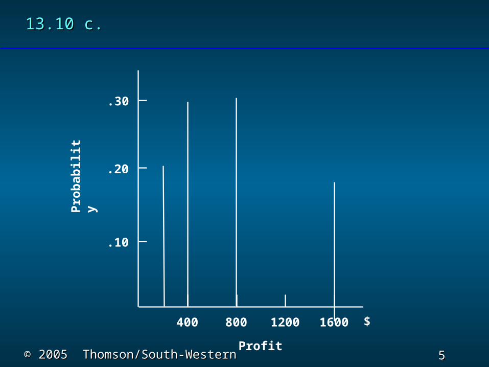
13.10 c.13.10 c.
Outcome and ProbabilityOutcome and Probability
$1600K : (0.4)(0.5)=0.2$1600K : (0.4)(0.5)=0.2 $800K : (0.6)(0.3)+(0.4)$800K : (0.6)(0.3)+(0.4)
(0.3)=0.3(0.3)=0.3 $400K : (0.6)(0.4)+(0.4)$400K : (0.6)(0.4)+(0.4)
(0.2)=0.32(0.2)=0.32 $200K : (0.6)(0.3)=0.18$200K : (0.6)(0.3)=0.18
5 5 Slide
Slide
© 2005 Thomson/South-Western© 2005 Thomson/South-Western
13.10 c.13.10 c.
.10
.20
.30
$400 800 1200 1600
Pro
bab
ilit
y
Profit
6 6 Slide
Slide
© 2005 Thomson/South-Western© 2005 Thomson/South-Western
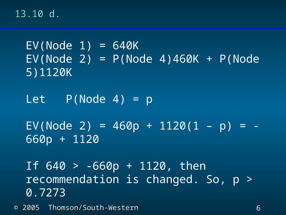
13.10 d.13.10 d.
EV(Node 1) = 640KEV(Node 2) = P(Node 4)460K + P(Node 5)1120K
Let P(Node 4) = p
EV(Node 2) = 460p + 1120(1 – p) = -660p + 1120
If 640 > -660p + 1120, then recommendation is changed. So, p > 0.7273
7 7 Slide
Slide
© 2005 Thomson/South-Western© 2005 Thomson/South-Western
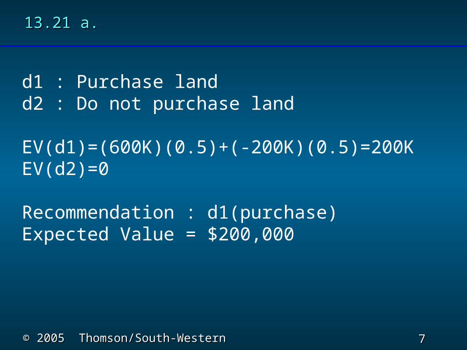
13.21 a.13.21 a.
d1 : Purchase landd2 : Do not purchase land
EV(d1)=(600K)(0.5)+(-200K)(0.5)=200KEV(d2)=0
Recommendation : d1(purchase) Expected Value = $200,000
8 8 Slide
Slide
© 2005 Thomson/South-Western© 2005 Thomson/South-Western
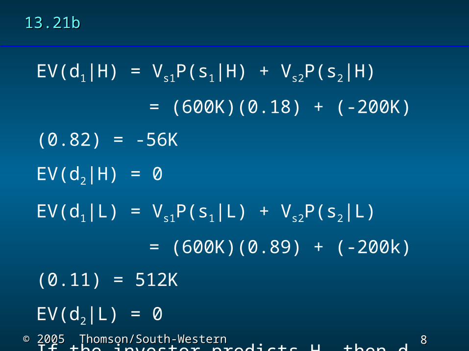
13.21b13.21b
EV(d1|H) = Vs1P(s1|H) + Vs2P(s2|H)
= (600K)(0.18) + (-200K)(0.82) = -56K
EV(d2|H) = 0
EV(d1|L) = Vs1P(s1|L) + Vs2P(s2|L)
= (600K)(0.89) + (-200k)(0.11) = 512K
EV(d2|L) = 0
If the investor predicts H, then d2 is selected with
EV(d2|H) = 0. Meanwhile, he predicts L, then d1 is
selected with EV(d1|L) = 512K
9 9 Slide
Slide
© 2005 Thomson/South-Western© 2005 Thomson/South-Western
13.21b13.21b
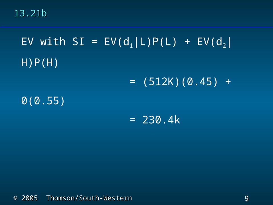
EV with SI = EV(d1|L)P(L) + EV(d2|H)P(H)
= (512K)(0.45) + 0(0.55)
= 230.4k
10 10 Slide
Slide
© 2005 Thomson/South-Western© 2005 Thomson/South-Western
13.21 c. 13.21 c.
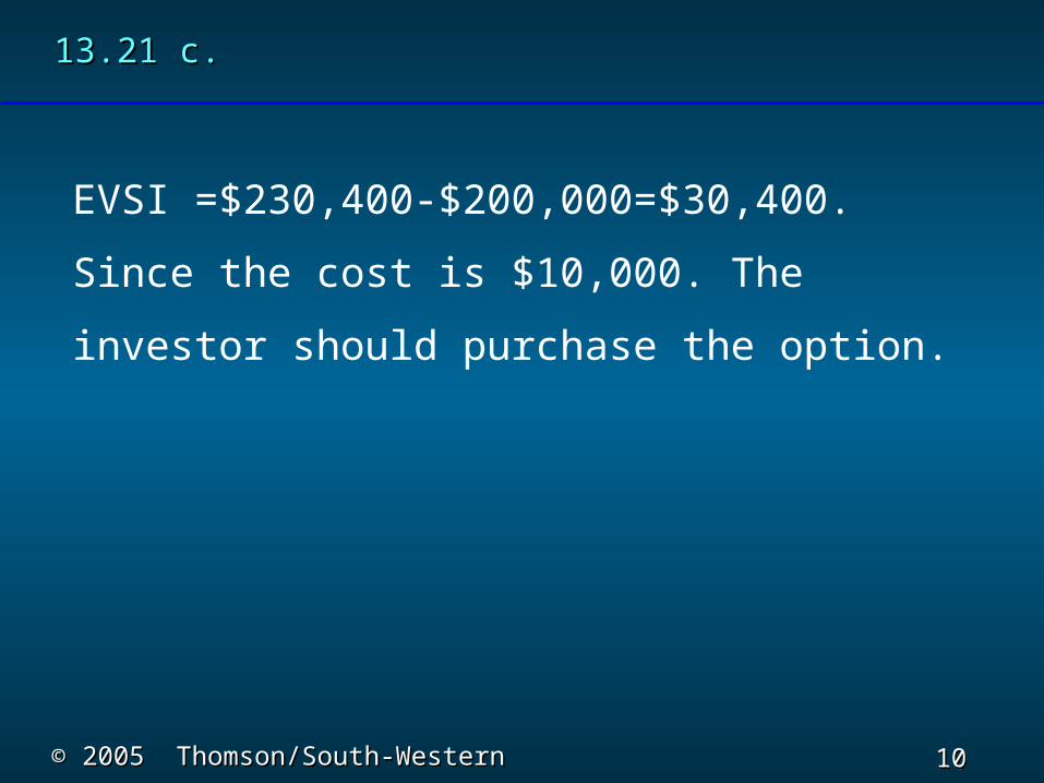
EVSI =$230,400-$200,000=$30,400. Since the
cost is $10,000. The investor should purchase
the option.

11 11 Slide
Slide
© 2005 Thomson/South-Western© 2005 Thomson/South-Western
Home WorkHome Work
14-314-314-1414-14
Due Day: Nov 18 (noon) 08Due Day: Nov 18 (noon) 08
12 12 Slide
Slide
© 2005 Thomson/South-Western© 2005 Thomson/South-Western
Chapter 14Chapter 14Multicriteria DecisionsMulticriteria Decisions
Goal ProgrammingGoal Programming Goal Programming: Formulation Goal Programming: Formulation Scoring ModelsScoring Models Analytic Hierarchy Process (AHP)Analytic Hierarchy Process (AHP) Establishing Priorities Using AHPEstablishing Priorities Using AHP Using AHP to Develop an Overall Using AHP to Develop an Overall
Priority RankingPriority Ranking
13 13 Slide
Slide
© 2005 Thomson/South-Western© 2005 Thomson/South-Western
Goal ProgrammingGoal Programming
Goal programmingGoal programming may be used to may be used to solve linear programs with multiple solve linear programs with multiple objectives, with each objective viewed objectives, with each objective viewed as a "goal". as a "goal".
In goal programming, In goal programming, ddii++ and and ddii
-- , , deviation variablesdeviation variables, are the amounts a , are the amounts a targeted goal targeted goal ii is overachieved or is overachieved or underachieved, respectively.underachieved, respectively.
The goals themselves are added to the The goals themselves are added to the constraint set with constraint set with ddii
++ and and ddii-- acting as acting as
the surplus and slack variables.the surplus and slack variables.
14 14 Slide
Slide
© 2005 Thomson/South-Western© 2005 Thomson/South-Western
Goal ProgrammingGoal Programming
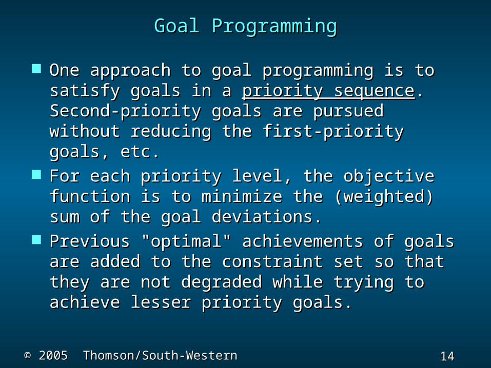
One approach to goal programming is to One approach to goal programming is to satisfy goals in a satisfy goals in a priority sequencepriority sequence. . Second-priority goals are pursued without Second-priority goals are pursued without reducing the first-priority goals, etc.reducing the first-priority goals, etc.
For each priority level, the objective For each priority level, the objective function is to minimize the (weighted) function is to minimize the (weighted) sum of the goal deviations. sum of the goal deviations.
Previous "optimal" achievements of goals Previous "optimal" achievements of goals are added to the constraint set so that are added to the constraint set so that they are not degraded while trying to they are not degraded while trying to achieve lesser priority goals. achieve lesser priority goals.
15 15 Slide
Slide
© 2005 Thomson/South-Western© 2005 Thomson/South-Western
Goal Programming FormulationGoal Programming Formulation
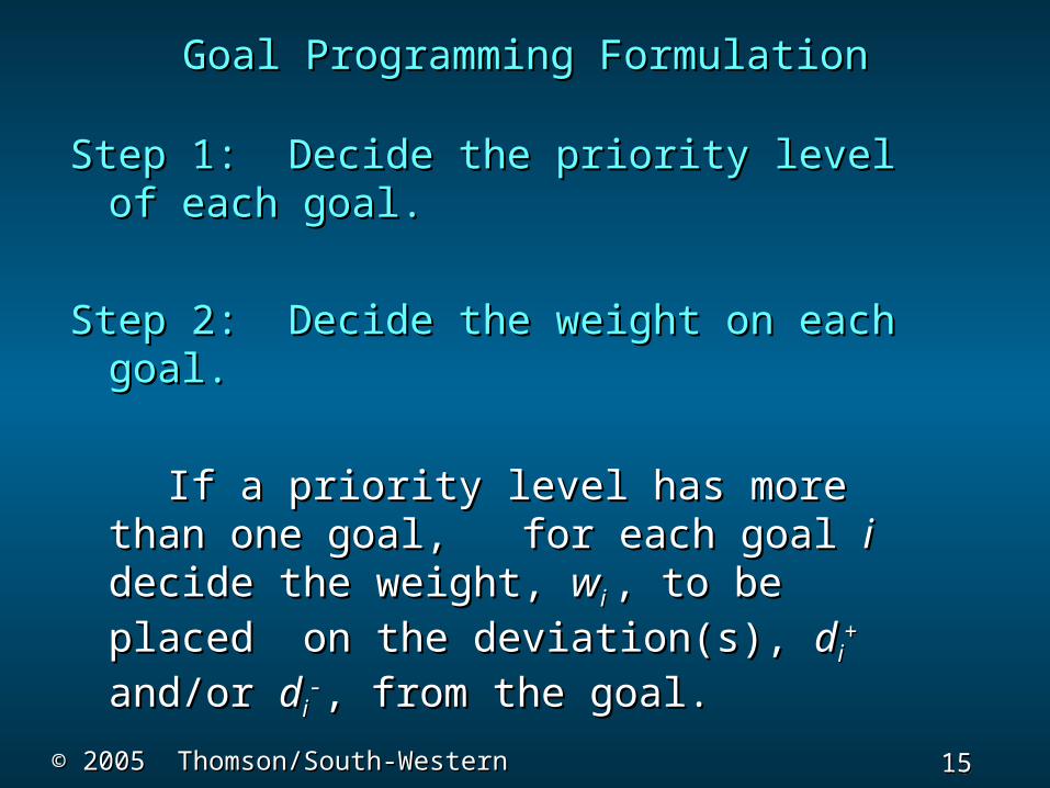
Step 1: Decide the priority level of each Step 1: Decide the priority level of each goal.goal.
Step 2: Decide the weight on each goal.Step 2: Decide the weight on each goal.
If a priority level has more than one If a priority level has more than one goal, for each goal goal, for each goal ii decide the decide the weight, weight, wwi i , to be placed on the , to be placed on the deviation(s), deviation(s), ddii
++ and/or and/or ddii--, from the , from the
goal.goal.
16 16 Slide
Slide
© 2005 Thomson/South-Western© 2005 Thomson/South-Western
Goal Programming FormulationGoal Programming Formulation
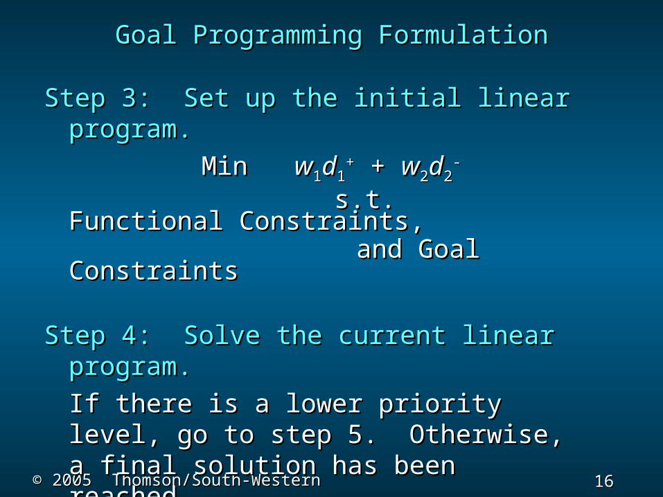
Step 3: Set up the initial linear program.Step 3: Set up the initial linear program.
Min Min ww11dd11++ + + ww22dd22
--
s.t. Functional Constraints, s.t. Functional Constraints, and Goal Constraints and Goal Constraints
Step 4: Solve the current linear program.Step 4: Solve the current linear program.
If there is a lower priority level, go to If there is a lower priority level, go to step 5. Otherwise, a final solution has step 5. Otherwise, a final solution has been reached.been reached.
17 17 Slide
Slide
© 2005 Thomson/South-Western© 2005 Thomson/South-Western
Goal Programming FormulationGoal Programming Formulation
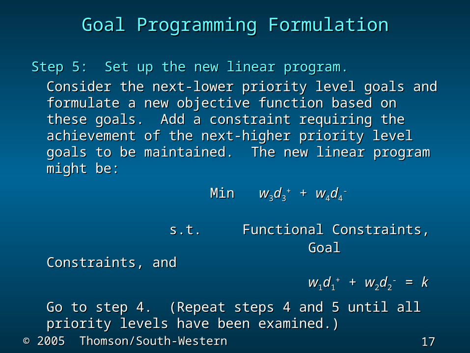
Step 5: Set up the new linear program.Step 5: Set up the new linear program.
Consider the next-lower priority level goals Consider the next-lower priority level goals and formulate a new objective function based on and formulate a new objective function based on these goals. Add a constraint requiring the these goals. Add a constraint requiring the achievement of the next-higher priority level achievement of the next-higher priority level goals to be maintained. goals to be maintained. The new linear The new linear program might be:program might be:
Min Min ww33dd33++ + + ww44dd44
--
s.t. Functional Constraints,s.t. Functional Constraints, Goal Constraints, andGoal Constraints, and
ww11dd11++ + + ww22dd22
-- = = kk
Go to step 4. (Repeat steps 4 and 5 until Go to step 4. (Repeat steps 4 and 5 until all priority levels have been examined.) all priority levels have been examined.)
18 18 Slide
Slide
© 2005 Thomson/South-Western© 2005 Thomson/South-Western
Example: Conceptual ProductsExample: Conceptual Products
Conceptual Products is a computer Conceptual Products is a computer company thatcompany that
produces the CP400 and CP500 computers. Theproduces the CP400 and CP500 computers. The
computers use differentcomputers use different
mother boards producedmother boards produced
in abundant supply by thein abundant supply by the
company, but use the samecompany, but use the same
cases and disk drives. Thecases and disk drives. The
CP400 models use two floppy disk drives and no CP400 models use two floppy disk drives and no zipzip
disk drives whereas the CP500 models use onedisk drives whereas the CP500 models use one
floppy disk drive and one zip disk drive.floppy disk drive and one zip disk drive.
19 19 Slide
Slide
© 2005 Thomson/South-Western© 2005 Thomson/South-Western
Example: Conceptual ProductsExample: Conceptual Products
The disk drives and cases are The disk drives and cases are boughtbought
from vendors. There are 1000 floppy from vendors. There are 1000 floppy disk drives, 500 zip disk drives, and disk drives, 500 zip disk drives, and 600 cases available to Conceptual 600 cases available to Conceptual Products on a weekly basis. It takes Products on a weekly basis. It takes one hour to manufacture a CP400 and one hour to manufacture a CP400 and its profit is $200 and it takes one and its profit is $200 and it takes one and one-half hours to manufacture a CP500 one-half hours to manufacture a CP500 and its profit is $500.and its profit is $500.
20 20 Slide
Slide
© 2005 Thomson/South-Western© 2005 Thomson/South-Western
Example: Conceptual ProductsExample: Conceptual Products
The company has four goals:The company has four goals:
Priority 1: Meet a state contract of 200 CP400 Priority 1: Meet a state contract of 200 CP400 machines weekly. (Goal 1) machines weekly. (Goal 1)
Priority 2: Make at least 500 total computers Priority 2: Make at least 500 total computers weekly. (Goal 2) weekly. (Goal 2)
Priority 3: Make at least $250,000 weekly. Priority 3: Make at least $250,000 weekly. (Goal 3)(Goal 3)
Priority 4: Use no more than 400 man-hours Priority 4: Use no more than 400 man-hours per per week. (Goal 4) week. (Goal 4)
21 21 Slide
Slide
© 2005 Thomson/South-Western© 2005 Thomson/South-Western
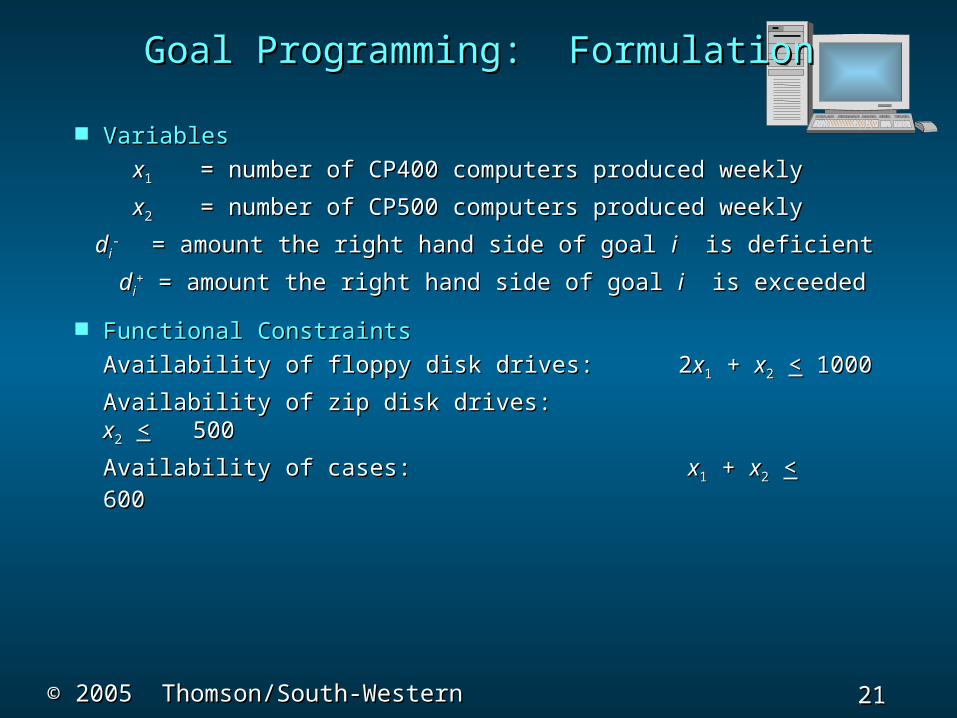
VariablesVariables
xx11 = number of CP400 computers produced weekly= number of CP400 computers produced weekly
xx22 = number of CP500 computers produced weekly= number of CP500 computers produced weekly
ddii- - = amount the right hand side of goal = amount the right hand side of goal ii is deficient is deficient
ddii++ = amount the right hand side of goal = amount the right hand side of goal ii is exceeded is exceeded
Functional ConstraintsFunctional Constraints
Availability of floppy disk drives: 2Availability of floppy disk drives: 2xx11 + + xx22 << 1000 1000
Availability of zip disk drives: Availability of zip disk drives: xx22 << 500 500
Availability of cases:Availability of cases: xx11 + + xx22 << 600 600
Goal Programming: FormulationGoal Programming: Formulation
22 22 Slide
Slide
© 2005 Thomson/South-Western© 2005 Thomson/South-Western
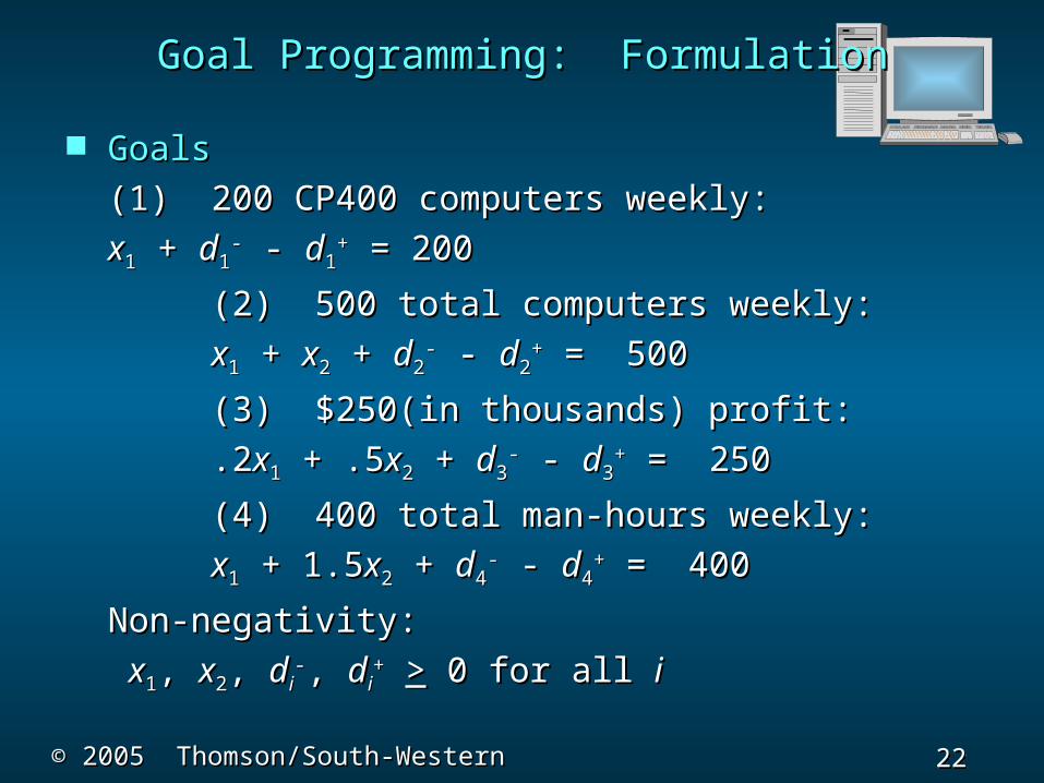
GoalsGoals
(1) 200 CP400 computers weekly: (1) 200 CP400 computers weekly:
xx11 + + dd11-- - - dd11
++ = 200 = 200
(2) 500 total computers weekly: (2) 500 total computers weekly:
xx11 + + xx22 + + dd22-- - - dd22
++ = 500 = 500
(3) $250(in thousands) profit:(3) $250(in thousands) profit:
.2.2xx11 + .5 + .5xx22 + + dd33-- - - dd33
++ = 250 = 250
(4) 400 total man-hours weekly: (4) 400 total man-hours weekly:
xx11 + 1.5 + 1.5xx22 + + dd44-- - - dd44
++ = 400 = 400
Non-negativity: Non-negativity:
xx11, , xx22, , ddii--, , ddii
++ >> 0 for all 0 for all ii
Goal Programming: FormulationGoal Programming: Formulation
23 23 Slide
Slide
© 2005 Thomson/South-Western© 2005 Thomson/South-Western
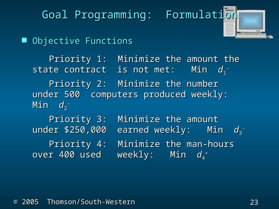
Objective FunctionsObjective Functions
Priority 1: Minimize the amount the state Priority 1: Minimize the amount the state contract contract is not met: Min is not met: Min dd11
--
Priority 2: Minimize the number under 500 Priority 2: Minimize the number under 500 computers produced weekly: computers produced weekly:
Min Min dd22--
Priority 3: Minimize the amount under Priority 3: Minimize the amount under $250,000 $250,000 earned weekly: Min earned weekly: Min dd33
--
Priority 4: Minimize the man-hours over 400 Priority 4: Minimize the man-hours over 400 used used weekly: Min weekly: Min dd44
++
Goal Programming: FormulationGoal Programming: Formulation
24 24 Slide
Slide
© 2005 Thomson/South-Western© 2005 Thomson/South-Western
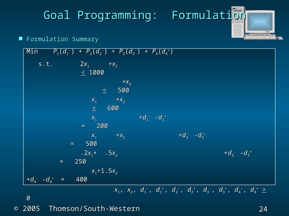
Formulation SummaryFormulation Summary
Min Min PP11((dd11--) + ) + PP22((dd22
--) + ) + PP33((dd33--) + ) + PP44((dd44
++))
s.t. 2s.t. 2xx11 + +xx22 << 1000 1000
++xx22 << 500 500
xx11 + +xx22 << 600 600
xx11 + +dd11-- - -dd11
++ = 200 = 200
xx11 + +xx22 + +dd22-- - -dd22
++ = 500 = 500
.2.2xx11+ .5+ .5xx22 + +dd33-- - -dd33
+ + = 250 = 250
xx11+1.5+1.5xx22 + +dd44-- - -dd44
+ + = 400= 400
xx11, , xx22, , dd11--, , dd11
++, , dd22--, , dd22
++, , dd33--, , dd33
++, , dd44--, , dd44
++ >> 0 0
Goal Programming: FormulationGoal Programming: Formulation
25 25 Slide
Slide
© 2005 Thomson/South-Western© 2005 Thomson/South-Western
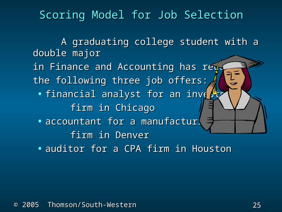
Scoring Model for Job SelectionScoring Model for Job Selection
A graduating college student with a A graduating college student with a double majordouble major
in Finance and Accounting has receivedin Finance and Accounting has received
the following three job offers:the following three job offers:
• financial analyst for an investmentfinancial analyst for an investment
firm in Chicagofirm in Chicago
• accountant for a manufacturingaccountant for a manufacturing
firm in Denverfirm in Denver
• auditor for a CPA firm in Houstonauditor for a CPA firm in Houston
26 26 Slide
Slide
© 2005 Thomson/South-Western© 2005 Thomson/South-Western
Scoring Model for Job SelectionScoring Model for Job Selection
The student made the following comments:The student made the following comments:
• ““The financial analyst positionThe financial analyst position
provides the best opportunity for myprovides the best opportunity for my
long-run career advancement.”long-run career advancement.”
• ““I would prefer living in DenverI would prefer living in Denver
rather than in Chicago or Houston.”rather than in Chicago or Houston.”
• ““I like the management style andI like the management style and
philosophy at the Houston CPA firmphilosophy at the Houston CPA firm
the best.”the best.” Clearly, this is a multicriteria decision.Clearly, this is a multicriteria decision.
27 27 Slide
Slide
© 2005 Thomson/South-Western© 2005 Thomson/South-Western
Scoring Model for Job SelectionScoring Model for Job Selection
Considering only the Considering only the long-run careerlong-run career
advancementadvancement criterion: criterion:
• The The financial analyst position infinancial analyst position in
ChicagoChicago is the best decision alternative. is the best decision alternative. Considering only the Considering only the locationlocation criterion: criterion:
• The The accountant position in Denveraccountant position in Denver
is the best decision alternative.is the best decision alternative. Considering only the Considering only the stylestyle criterion: criterion:
• The The auditor position in Houstonauditor position in Houston is is the best the best alternative.alternative.
28 28 Slide
Slide
© 2005 Thomson/South-Western© 2005 Thomson/South-Western
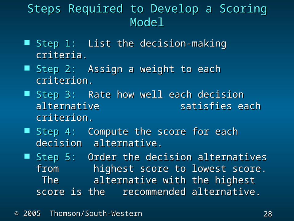
Steps Required to Develop a Scoring Steps Required to Develop a Scoring ModelModel
Step 1:Step 1: List the decision-making criteria. List the decision-making criteria. Step 2:Step 2: Assign a weight to each criterion. Assign a weight to each criterion. Step 3:Step 3: Rate how well each decision Rate how well each decision
alternative alternative satisfies each criterion.satisfies each criterion. Step 4:Step 4: Compute the score for each decision Compute the score for each decision
alternative.alternative. Step 5:Step 5: Order the decision alternatives from Order the decision alternatives from
highest score to lowest highest score to lowest score. The score. The alternative with the alternative with the highest score is the highest score is the recommended alternative.recommended alternative.
29 29 Slide
Slide
© 2005 Thomson/South-Western© 2005 Thomson/South-Western
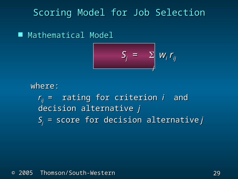
Mathematical ModelMathematical Model
SSjj = = wwii r rijij
ii
where:where:
rrijij = rating for criterion = rating for criterion ii and decision and decision alternative alternative jj
SSjj = = score for decision alternativescore for decision alternative j j
Scoring Model for Job SelectionScoring Model for Job Selection
30 30 Slide
Slide
© 2005 Thomson/South-Western© 2005 Thomson/South-Western
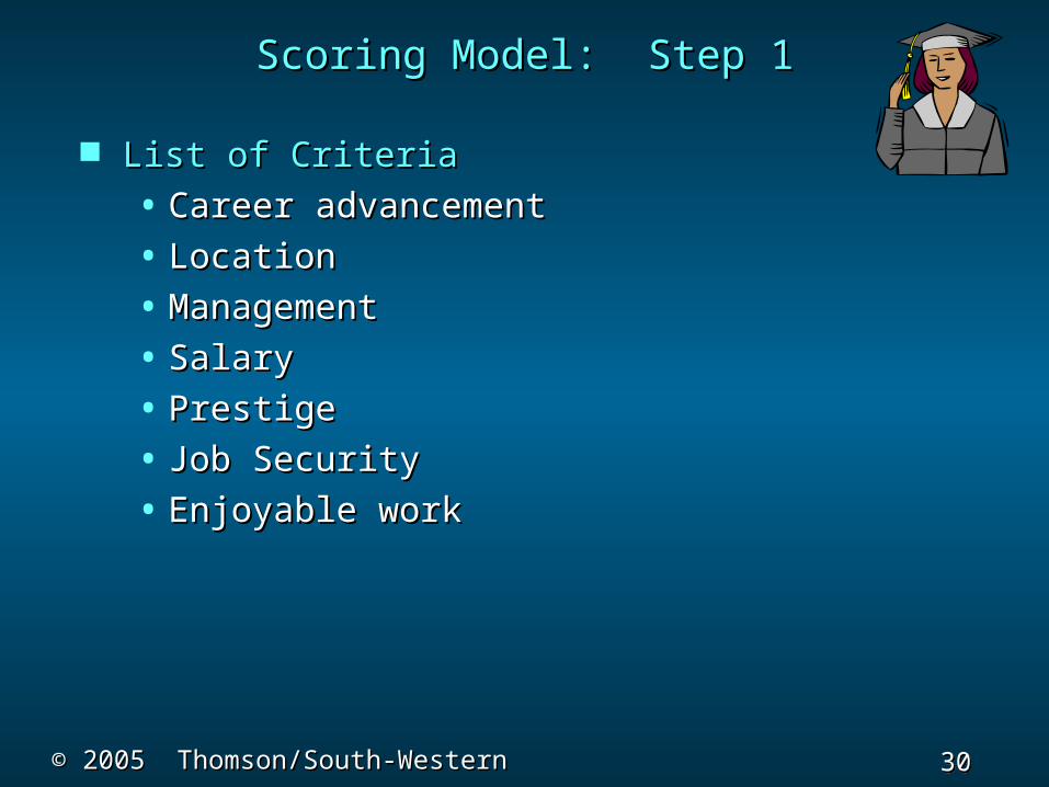
Scoring Model: Step 1Scoring Model: Step 1
List of CriteriaList of Criteria
• Career advancement Career advancement
• LocationLocation
• ManagementManagement
• SalarySalary
• PrestigePrestige
• Job SecurityJob Security
• Enjoyable workEnjoyable work
31 31 Slide
Slide
© 2005 Thomson/South-Western© 2005 Thomson/South-Western
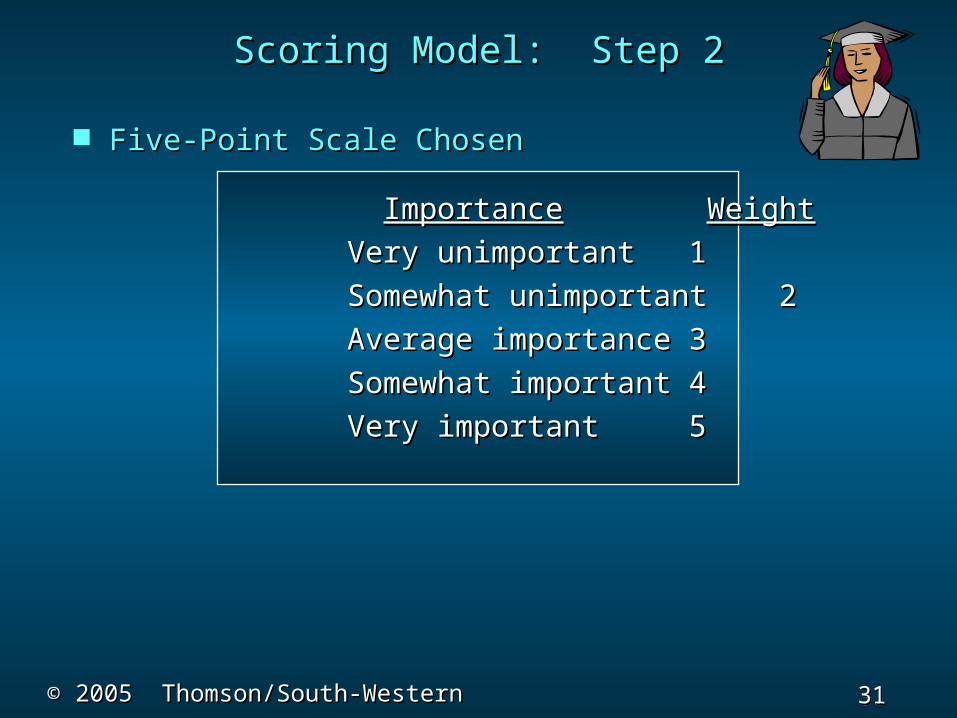
Scoring Model: Step 2Scoring Model: Step 2
Five-Point Scale ChosenFive-Point Scale Chosen
ImportanceImportance WeightWeight
Very unimportantVery unimportant 11
Somewhat unimportantSomewhat unimportant 22
Average importanceAverage importance 33
Somewhat importantSomewhat important 44
Very importantVery important 55
32 32 Slide
Slide
© 2005 Thomson/South-Western© 2005 Thomson/South-Western
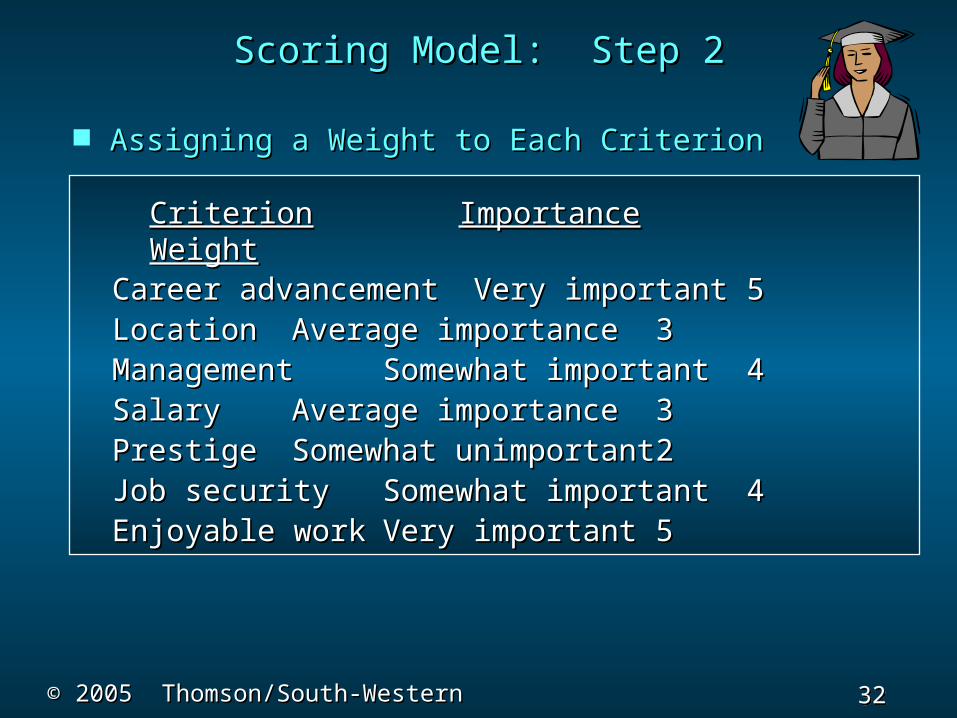
Scoring Model: Step 2Scoring Model: Step 2
Assigning a Weight to Each CriterionAssigning a Weight to Each Criterion
CriterionCriterion ImportanceImportance WeightWeight Career advancementCareer advancement Very importantVery important 55 LocationLocation Average importanceAverage importance 33 ManagementManagement Somewhat importantSomewhat important 44 SalarySalary Average importanceAverage importance 33 PrestigePrestige Somewhat unimportantSomewhat unimportant 22 Job securityJob security Somewhat importantSomewhat important 44 Enjoyable workEnjoyable work Very importantVery important 55
33 33 Slide
Slide
© 2005 Thomson/South-Western© 2005 Thomson/South-Western
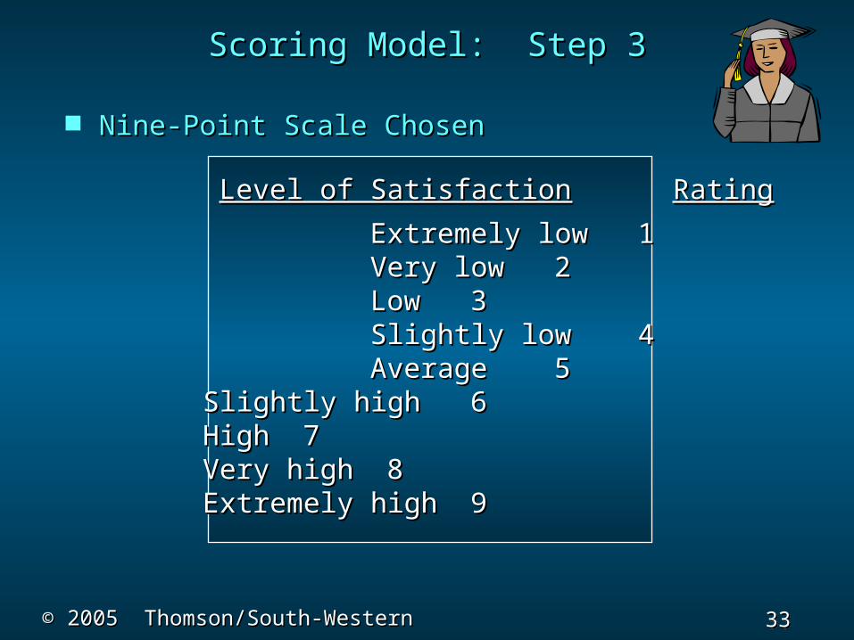
Nine-Point Scale ChosenNine-Point Scale Chosen
Level of SatisfactionLevel of Satisfaction RatingRating
Extremely lowExtremely low 11 Very lowVery low 22 LowLow 33 Slightly lowSlightly low 44 AverageAverage 55
Slightly highSlightly high 66 HighHigh 77 Very highVery high 88 Extremely highExtremely high 99
Scoring Model: Step 3Scoring Model: Step 3
34 34 Slide
Slide
© 2005 Thomson/South-Western© 2005 Thomson/South-Western
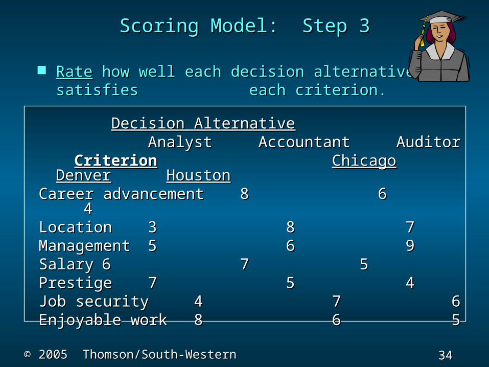
RateRate how well each decision alternative satisfies how well each decision alternative satisfies each criterion. each criterion.
Decision AlternativeDecision Alternative Analyst AccountantAnalyst Accountant
AuditorAuditor CriterionCriterion ChicagoChicago DenverDenver HoustonHouston
Career advancementCareer advancement 88 6 6 4 4LocationLocation 33 8 8 7 7ManagementManagement 55 6 6 9 9SalarySalary 66 7 7 5 5PrestigePrestige 77 5 5 4 4Job securityJob security 44 7 7 6 6Enjoyable workEnjoyable work 88 6 6 5 5
Scoring Model: Step 3Scoring Model: Step 3
35 35 Slide
Slide
© 2005 Thomson/South-Western© 2005 Thomson/South-Western
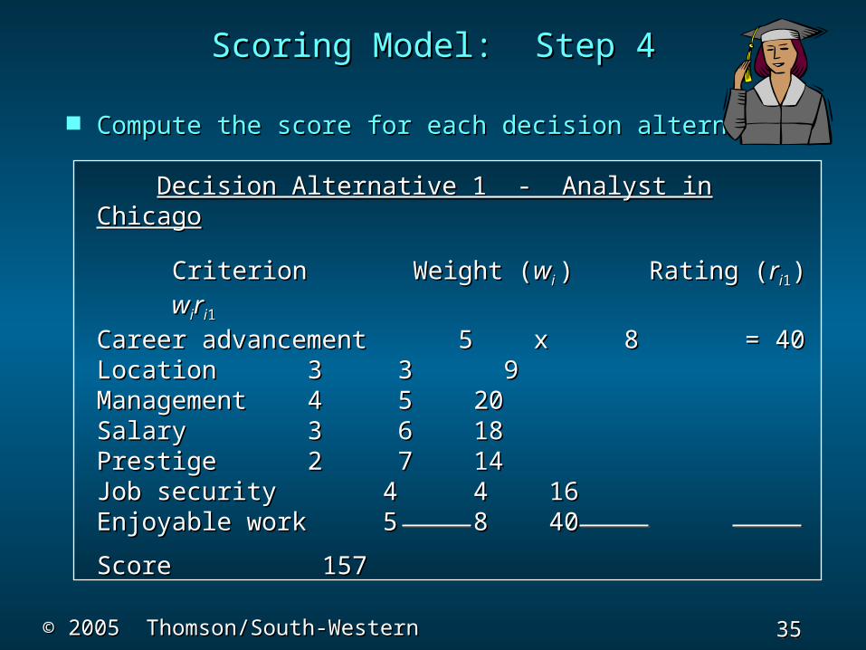
Compute the score for each decision alternative.Compute the score for each decision alternative.
Decision Alternative 1 - Analyst in ChicagoDecision Alternative 1 - Analyst in Chicago
CriterionCriterion Weight ( Weight (wwi i ) Rating () Rating (rrii11) ) wwiirrii11
Career advancementCareer advancement 5 5 x x 8 8 = = 4040LocationLocation 3 3 3 3 9 9ManagementManagement 4 4 5 5 2020SalarySalary 3 3 6 6 1818PrestigePrestige 2 2 7 7 1414Job securityJob security 4 4 4 4 1616Enjoyable workEnjoyable work 5 5 8 8 4040
ScoreScore 157 157
Scoring Model: Step 4Scoring Model: Step 4
36 36 Slide
Slide
© 2005 Thomson/South-Western© 2005 Thomson/South-Western
Compute the score for each decision alternative.Compute the score for each decision alternative.
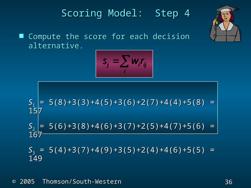
SS11 = = 5(8)+3(3)+4(5)+3(6)+2(7)+4(4)+5(8) = 1575(8)+3(3)+4(5)+3(6)+2(7)+4(4)+5(8) = 157
SS22 = = 5(6)+3(8)+4(6)+3(7)+2(5)+4(7)+5(6) = 1675(6)+3(8)+4(6)+3(7)+2(5)+4(7)+5(6) = 167
SS33 = = 5(4)+3(7)+4(9)+3(5)+2(4)+4(6)+5(5) = 1495(4)+3(7)+4(9)+3(5)+2(4)+4(6)+5(5) = 149
j i iji
s wrj i iji
s wr
Scoring Model: Step 4Scoring Model: Step 4
37 37 Slide
Slide
© 2005 Thomson/South-Western© 2005 Thomson/South-Western
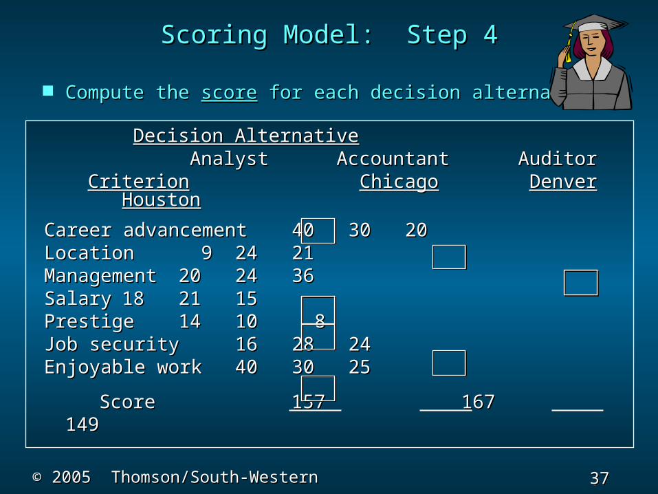
Compute the Compute the scorescore for each decision alternative. for each decision alternative.
Decision AlternativeDecision Alternative Analyst AccountantAnalyst Accountant
AuditorAuditor CriterionCriterion ChicagoChicago DenverDenver HoustonHouston
Career advancementCareer advancement 4040 3030 2020LocationLocation 9 9 2424 2121ManagementManagement 2020 2424 3636SalarySalary 1818 2121 1515PrestigePrestige 1414 1010 8 8Job securityJob security 1616 2828 2424Enjoyable workEnjoyable work 4040 3030 2525
ScoreScore 157 157 167 167 149 149
Scoring Model: Step 4Scoring Model: Step 4
38 38 Slide
Slide
© 2005 Thomson/South-Western© 2005 Thomson/South-Western
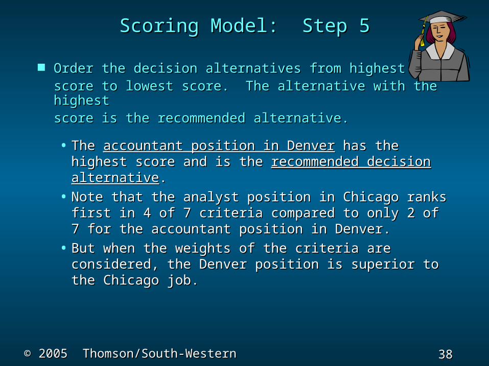
Order the decision alternatives from highestOrder the decision alternatives from highestscore to lowest score. The alternative with the score to lowest score. The alternative with the highesthighestscore is the recommended alternative.score is the recommended alternative.
• The The accountant position in Denveraccountant position in Denver has the has the highest score and is the highest score and is the recommended decision recommended decision alternativealternative..
• Note that the analyst position in Chicago ranks Note that the analyst position in Chicago ranks first in 4 of 7 criteria compared to only 2 of 7 for first in 4 of 7 criteria compared to only 2 of 7 for the accountant position in Denver.the accountant position in Denver.
• But when the weights of the criteria are But when the weights of the criteria are considered, the Denver position is superior to the considered, the Denver position is superior to the Chicago job.Chicago job.
Scoring Model: Step 5Scoring Model: Step 5
39 39 Slide
Slide
© 2005 Thomson/South-Western© 2005 Thomson/South-Western
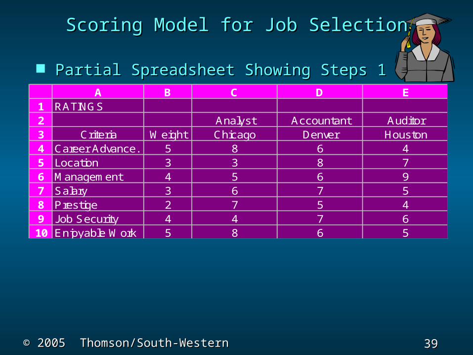
Scoring Model for Job SelectionScoring Model for Job Selection
Partial Spreadsheet Showing Steps 1 - 3Partial Spreadsheet Showing Steps 1 - 3A B C D E
1 RATINGS2 Analyst Accountant Auditor3 Criteria Weight Chicago Denver Houston4 Career Advance. 5 8 6 45 Location 3 3 8 76 Management 4 5 6 97 Salary 3 6 7 58 Prestige 2 7 5 49 Job Security 4 4 7 610 Enjoyable Work 5 8 6 5
40 40 Slide
Slide
© 2005 Thomson/South-Western© 2005 Thomson/South-Western
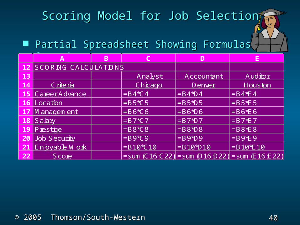
Scoring Model for Job SelectionScoring Model for Job Selection
Partial Spreadsheet Showing Formulas of Step 4Partial Spreadsheet Showing Formulas of Step 4 A B C D E
12 SCORING CALCULATIONS13 Analyst Accountant Auditor14 Criteria Chicago Denver Houston15 Career Advance. =B4*C4 =B4*D4 =B4*E416 Location =B5*C5 =B5*D5 =B5*E517 Management =B6*C6 =B6*D6 =B6*E618 Salary =B7*C7 =B7*D7 =B7*E719 Prestige =B8*C8 =B8*D8 =B8*E820 Job Security =B9*C9 =B9*D9 =B9*E921 Enjoyable Work =B10*C10 =B10*D10 =B10*E1022 Score =sum(C16:C22) =sum(D16:D22) =sum(E16:E22)
41 41 Slide
Slide
© 2005 Thomson/South-Western© 2005 Thomson/South-Western
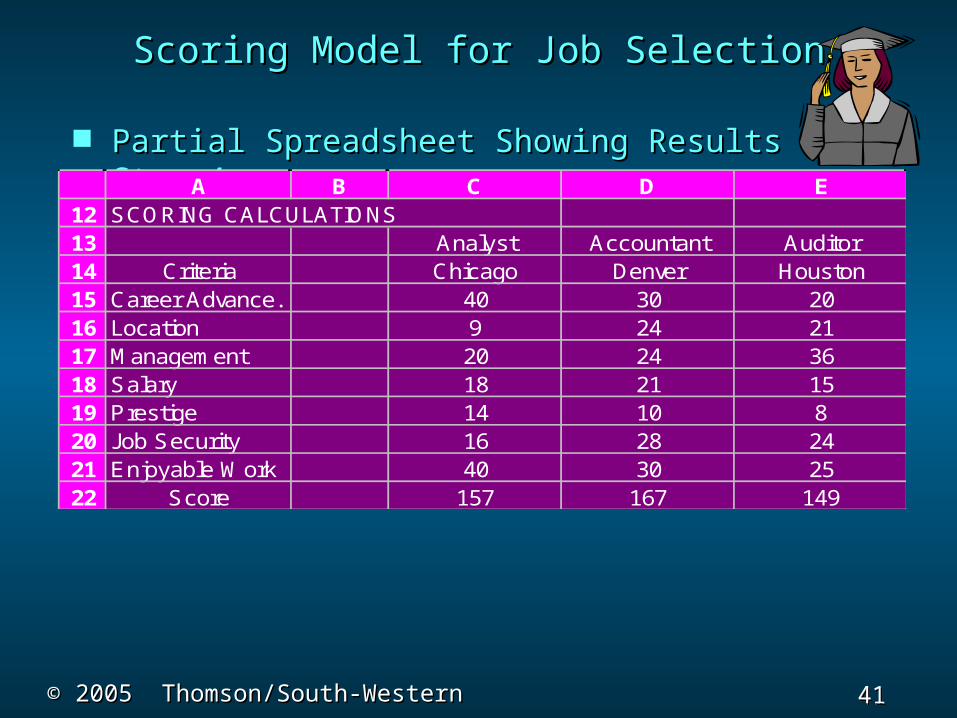
Scoring Model for Job SelectionScoring Model for Job Selection
Partial Spreadsheet Showing Results of Step 4Partial Spreadsheet Showing Results of Step 4 A B C D E
12 SCORING CALCULATIONS13 Analyst Accountant Auditor14 Criteria Chicago Denver Houston15 Career Advance. 40 30 2016 Location 9 24 2117 Management 20 24 3618 Salary 18 21 1519 Prestige 14 10 820 Job Security 16 28 2421 Enjoyable Work 40 30 2522 Score 157 167 149
42 42 Slide
Slide
© 2005 Thomson/South-Western© 2005 Thomson/South-Western
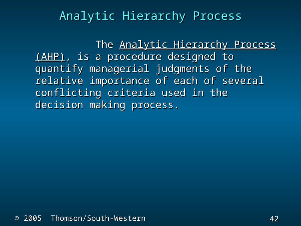
Analytic Hierarchy ProcessAnalytic Hierarchy Process
The The Analytic Hierarchy Process (AHP)Analytic Hierarchy Process (AHP), is a , is a procedure designed to quantify managerial procedure designed to quantify managerial judgments of the relative importance of each of judgments of the relative importance of each of several conflicting criteria used in the decision several conflicting criteria used in the decision making process.making process.
43 43 Slide
Slide
© 2005 Thomson/South-Western© 2005 Thomson/South-Western
Analytic Hierarchy ProcessAnalytic Hierarchy Process
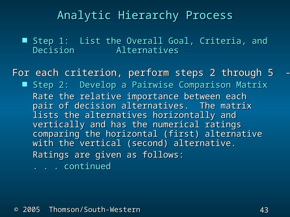
Step 1: List the Overall Goal, Criteria, and Step 1: List the Overall Goal, Criteria, and Decision Decision Alternatives Alternatives
Step 2: Develop a Pairwise Comparison MatrixStep 2: Develop a Pairwise Comparison MatrixRate the relative importance between each Rate the relative importance between each
pair of decision alternatives. The matrix lists the pair of decision alternatives. The matrix lists the alternatives horizontally and vertically and has the alternatives horizontally and vertically and has the numerical ratings comparing the horizontal (first) numerical ratings comparing the horizontal (first) alternative with the vertical (second) alternative.alternative with the vertical (second) alternative.
Ratings are given as follows:Ratings are given as follows: . . . continued. . . continued
------- For each criterion, perform steps 2 through 5 -------------- For each criterion, perform steps 2 through 5 -------------- For each criterion, perform steps 2 through 5 -------------- For each criterion, perform steps 2 through 5 -------
44 44 Slide
Slide
© 2005 Thomson/South-Western© 2005 Thomson/South-Western
Analytic Hierarchy ProcessAnalytic Hierarchy Process
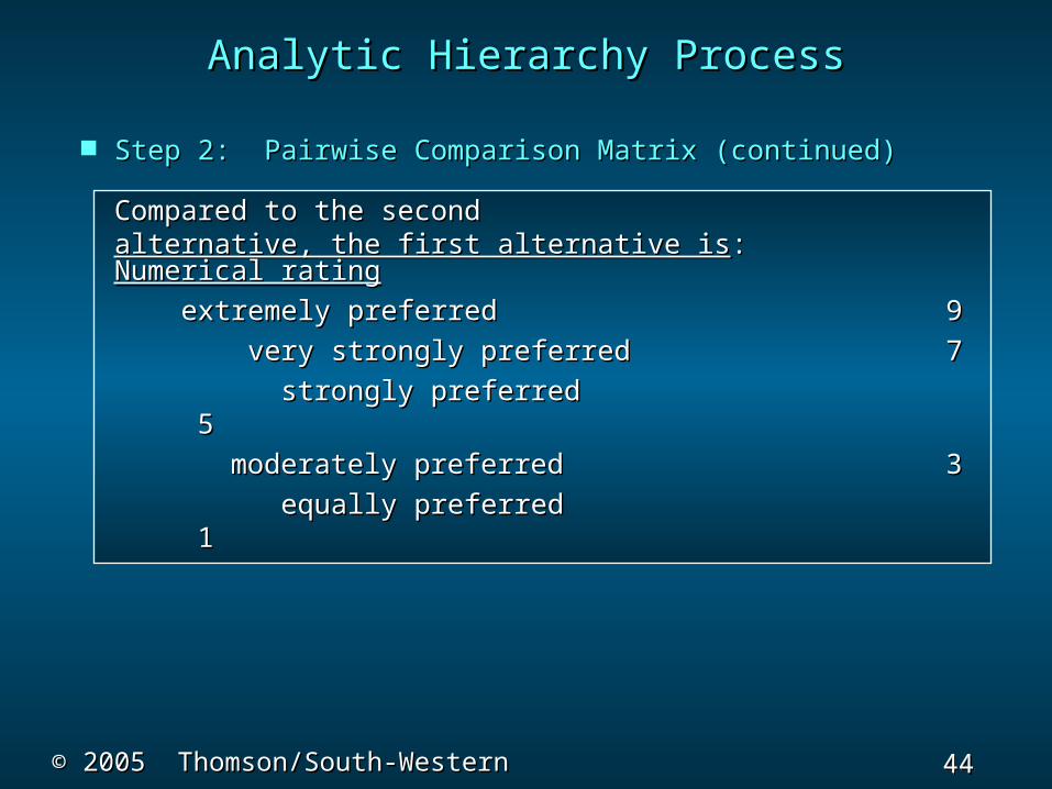
Step 2: Pairwise Comparison Matrix (continued)Step 2: Pairwise Comparison Matrix (continued)
Compared to the secondCompared to the secondalternative, the first alternative isalternative, the first alternative is: : Numerical Numerical ratingrating
extremely preferred extremely preferred 99
very strongly preferred very strongly preferred 77
strongly preferred strongly preferred 55
moderately preferred moderately preferred 33
equally preferred equally preferred 11
45 45 Slide
Slide
© 2005 Thomson/South-Western© 2005 Thomson/South-Western
Analytic Hierarchy ProcessAnalytic Hierarchy Process
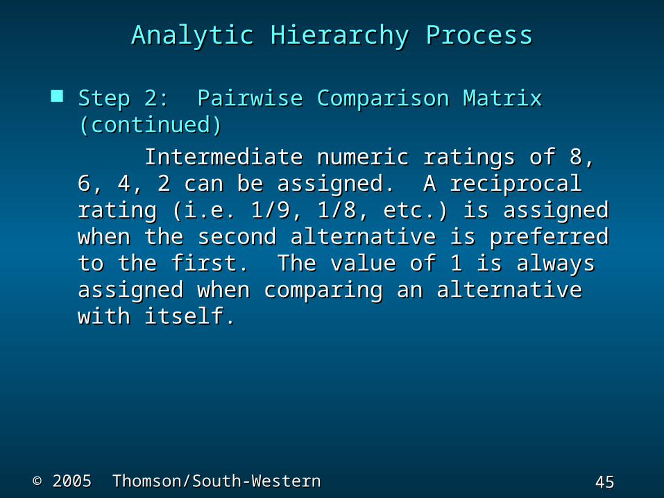
Step 2: Pairwise Comparison Matrix (continued)Step 2: Pairwise Comparison Matrix (continued)
Intermediate numeric ratings of 8, 6, 4, 2 Intermediate numeric ratings of 8, 6, 4, 2 can be assigned. A reciprocal rating (i.e. 1/9, can be assigned. A reciprocal rating (i.e. 1/9, 1/8, etc.) is assigned when the second 1/8, etc.) is assigned when the second alternative is preferred to the first. The value alternative is preferred to the first. The value of 1 is always assigned when comparing an of 1 is always assigned when comparing an alternative with itself. alternative with itself.
46 46 Slide
Slide
© 2005 Thomson/South-Western© 2005 Thomson/South-Western
Analytic Hierarchy ProcessAnalytic Hierarchy Process
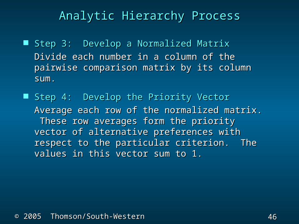
Step 3: Develop a Normalized MatrixStep 3: Develop a Normalized Matrix
Divide each number in a column of the Divide each number in a column of the pairwise comparison matrix by its column pairwise comparison matrix by its column sum.sum.
Step 4: Develop the Priority VectorStep 4: Develop the Priority Vector
Average each row of the normalized Average each row of the normalized matrix. These row averages form the priority matrix. These row averages form the priority vector of alternative preferences with respect vector of alternative preferences with respect to the particular criterion. The values in this to the particular criterion. The values in this vector sum to 1.vector sum to 1.
47 47 Slide
Slide
© 2005 Thomson/South-Western© 2005 Thomson/South-Western
Analytic Hierarchy ProcessAnalytic Hierarchy Process
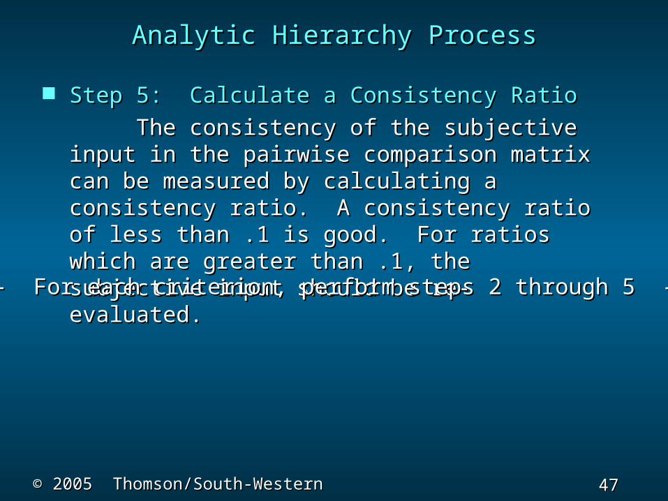
Step 5: Calculate a Consistency RatioStep 5: Calculate a Consistency Ratio
The consistency of the subjective input The consistency of the subjective input in the pairwise comparison matrix can be in the pairwise comparison matrix can be measured by calculating a consistency ratio. A measured by calculating a consistency ratio. A consistency ratio of less than .1 is good. For consistency ratio of less than .1 is good. For ratios which are greater than .1, the subjective ratios which are greater than .1, the subjective input should be re-evaluated.input should be re-evaluated.
------- For each criterion, perform steps 2 through 5 -------------- For each criterion, perform steps 2 through 5 -------
48 48 Slide
Slide
© 2005 Thomson/South-Western© 2005 Thomson/South-Western
Analytic Hierarchy ProcessAnalytic Hierarchy Process
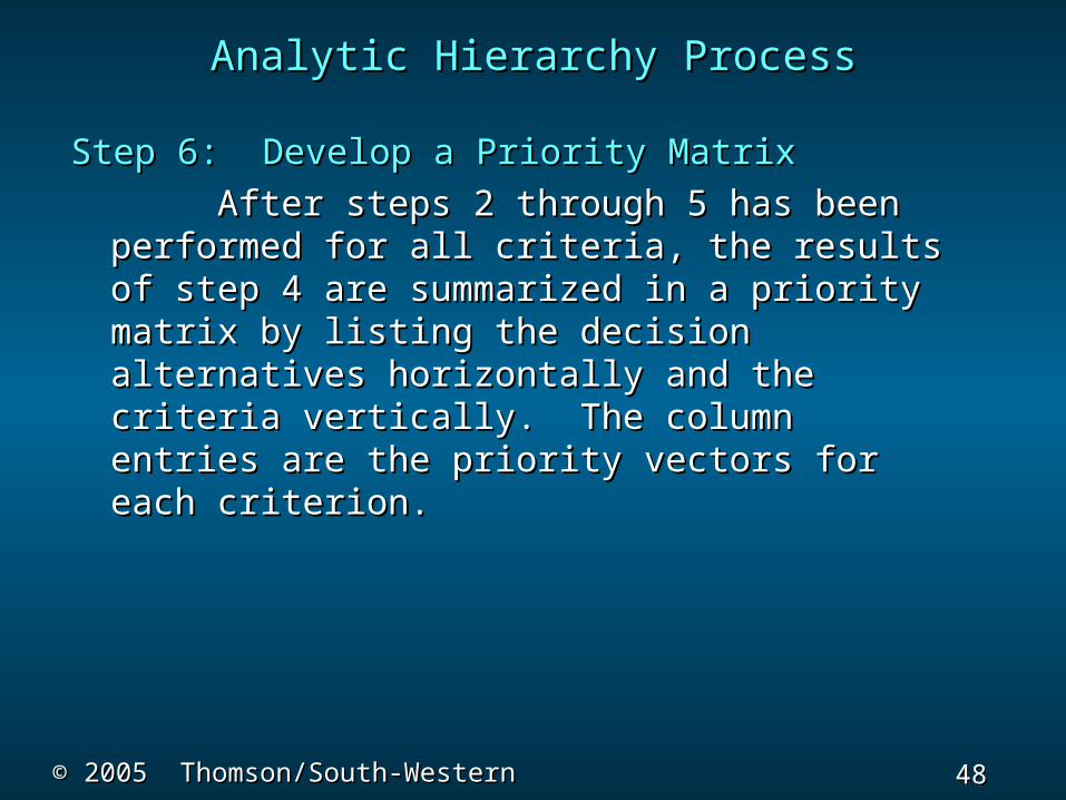
Step 6: Develop a Priority MatrixStep 6: Develop a Priority Matrix
After steps 2 through 5 has been After steps 2 through 5 has been performed for all criteria, the results of step 4 performed for all criteria, the results of step 4 are summarized in a priority matrix by listing are summarized in a priority matrix by listing the decision alternatives horizontally and the the decision alternatives horizontally and the criteria vertically. The column entries are the criteria vertically. The column entries are the priority vectors for each criterion. priority vectors for each criterion.
49 49 Slide
Slide
© 2005 Thomson/South-Western© 2005 Thomson/South-Western
Analytic Hierarchy ProcessAnalytic Hierarchy Process
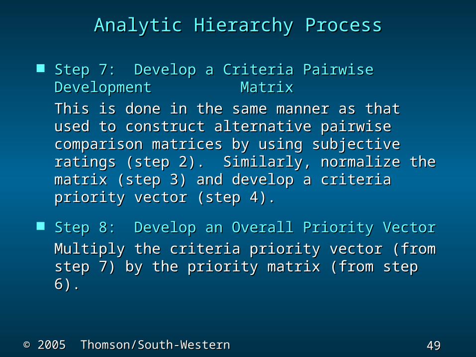
Step 7: Develop a Criteria Pairwise Step 7: Develop a Criteria Pairwise Development Development Matrix Matrix
This is done in the same manner as that This is done in the same manner as that used to construct alternative pairwise used to construct alternative pairwise comparison matrices by using subjective comparison matrices by using subjective ratings (step 2). Similarly, normalize the matrix ratings (step 2). Similarly, normalize the matrix (step 3) and develop a criteria priority vector (step 3) and develop a criteria priority vector (step 4). (step 4).
Step 8: Develop an Overall Priority VectorStep 8: Develop an Overall Priority Vector
Multiply the criteria priority vector (from Multiply the criteria priority vector (from step 7) by the priority matrix (from step 6).step 7) by the priority matrix (from step 6).
50 50 Slide
Slide
© 2005 Thomson/South-Western© 2005 Thomson/South-Western
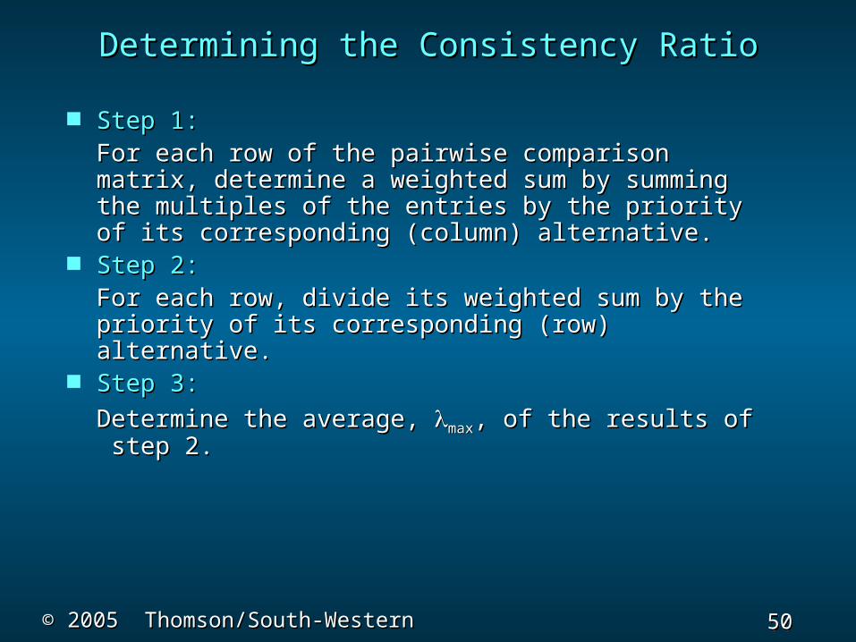
Determining the Consistency RatioDetermining the Consistency Ratio
Step 1:Step 1: For each row of the pairwise comparison For each row of the pairwise comparison
matrix, determine a weighted sum by summing matrix, determine a weighted sum by summing the multiples of the entries by the priority of its the multiples of the entries by the priority of its corresponding (column) alternative.corresponding (column) alternative.
Step 2:Step 2: For each row, divide its weighted sum by For each row, divide its weighted sum by
the priority of its corresponding (row) the priority of its corresponding (row) alternative.alternative.
Step 3:Step 3:
Determine the average, Determine the average, maxmax, of the results , of the results of step 2.of step 2.
51 51 Slide
Slide
© 2005 Thomson/South-Western© 2005 Thomson/South-Western
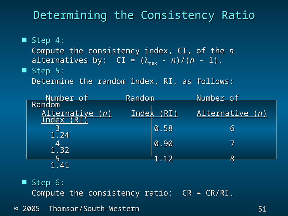
Step 4:Step 4: Compute the consistency index, CI, of the Compute the consistency index, CI, of the nn
alternatives by: CI = (alternatives by: CI = (maxmax - - nn)/()/(nn - 1). - 1). Step 5:Step 5:
Determine the random index, RI, as follows:Determine the random index, RI, as follows:
Number of Random Number of RandomNumber of Random Number of Random Alternative (Alternative (nn)) Index (RI)Index (RI) Alternative (Alternative (nn)) Index (RI)Index (RI)
3 0.583 0.58 6 6 1.24 1.24 4 0.904 0.90 7 7 1.32 1.32 5 1.125 1.12 8 8 1.41 1.41
Step 6:Step 6:Compute the consistency ratio: CR = CR/RI.Compute the consistency ratio: CR = CR/RI.
Determining the Consistency RatioDetermining the Consistency Ratio
52 52 Slide
Slide
© 2005 Thomson/South-Western© 2005 Thomson/South-Western
Example: Gill GlassExample: Gill Glass
Designer Gill Glass must decideDesigner Gill Glass must decide
which of three manufacturerswhich of three manufacturers
will develop his "signature“will develop his "signature“
toothbrushes. Three factorstoothbrushes. Three factors
are important to Gill: (1) his costs;are important to Gill: (1) his costs;
(2) reliability of the product; and, (3) delivery time(2) reliability of the product; and, (3) delivery time
of the orders.of the orders.The three manufacturers are Cornell The three manufacturers are Cornell
Industries,Industries, Brush Pik, and Picobuy. Cornell Industries will sellBrush Pik, and Picobuy. Cornell Industries will selltoothbrushes to Gill Glass for $100 per gross, toothbrushes to Gill Glass for $100 per gross, BrushBrushPik for $80 per gross, and Picobuy for $144 per Pik for $80 per gross, and Picobuy for $144 per gross.gross.
53 53 Slide
Slide
© 2005 Thomson/South-Western© 2005 Thomson/South-Western
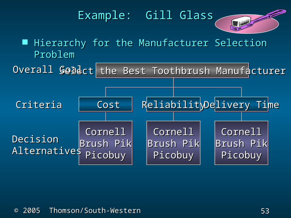
Example: Gill GlassExample: Gill Glass
Hierarchy for the Manufacturer Selection Hierarchy for the Manufacturer Selection ProblemProblem
Select the Best Toothbrush ManufacturerSelect the Best Toothbrush ManufacturerSelect the Best Toothbrush ManufacturerSelect the Best Toothbrush Manufacturer
CostCost CostCost ReliabilityReliabilityReliabilityReliability Delivery TimeDelivery TimeDelivery TimeDelivery Time
CornellCornellBrush PikBrush PikPicobuyPicobuy
CornellCornellBrush PikBrush PikPicobuyPicobuy
CornellCornellBrush PikBrush PikPicobuyPicobuy
CornellCornellBrush PikBrush PikPicobuyPicobuy
CornellCornellBrush PikBrush PikPicobuyPicobuy
CornellCornellBrush PikBrush PikPicobuyPicobuy
Overall GoalOverall Goal
CriteriaCriteria
DecisionDecisionAlternativesAlternatives
54 54 Slide
Slide
© 2005 Thomson/South-Western© 2005 Thomson/South-Western
Pairwise Comparison Matrix:Pairwise Comparison Matrix:CostCost
Gill has decided that in terms of price, Gill has decided that in terms of price, BrushBrushPik is moderately preferred to Cornell and Pik is moderately preferred to Cornell and veryverystrongly preferred to Picobuy. In turn Cornell strongly preferred to Picobuy. In turn Cornell isisstrongly to very strongly preferred to strongly to very strongly preferred to Picobuy.Picobuy.
55 55 Slide
Slide
© 2005 Thomson/South-Western© 2005 Thomson/South-Western
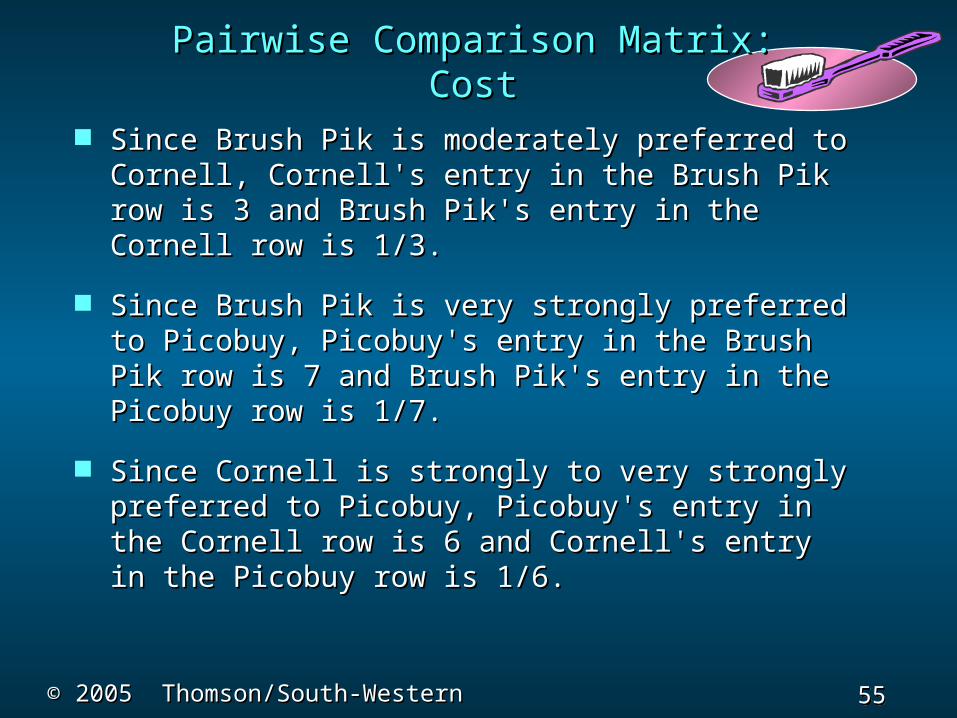
Since Brush Pik is moderately preferred to Since Brush Pik is moderately preferred to Cornell, Cornell's entry in the Brush Pik row is Cornell, Cornell's entry in the Brush Pik row is 3 and Brush Pik's entry in the Cornell row is 3 and Brush Pik's entry in the Cornell row is 1/3.1/3.
Since Brush Pik is very strongly preferred to Since Brush Pik is very strongly preferred to Picobuy, Picobuy's entry in the Brush Pik row Picobuy, Picobuy's entry in the Brush Pik row is 7 and Brush Pik's entry in the Picobuy row is 7 and Brush Pik's entry in the Picobuy row is 1/7.is 1/7.
Since Cornell is strongly to very strongly Since Cornell is strongly to very strongly preferred to Picobuy, Picobuy's entry in the preferred to Picobuy, Picobuy's entry in the Cornell row is 6 and Cornell's entry in the Cornell row is 6 and Cornell's entry in the Picobuy row is 1/6.Picobuy row is 1/6.
Pairwise Comparison Matrix:Pairwise Comparison Matrix:CostCost
56 56 Slide
Slide
© 2005 Thomson/South-Western© 2005 Thomson/South-Western
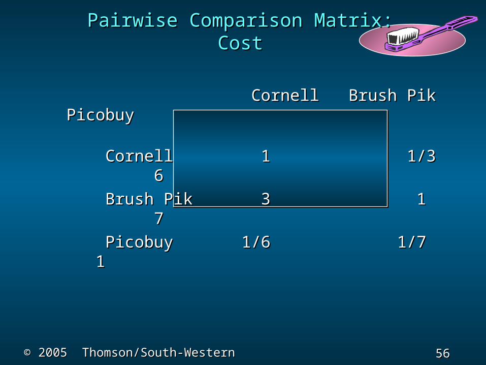
Cornell Brush Pik PicobuyCornell Brush Pik Picobuy
CornellCornell 1 1/3 1 1/3 6 6
Brush PikBrush Pik 3 3 1 1 7 7
PicobuyPicobuy 1/6 1/6 1/7 1/7 1 1
Pairwise Comparison Matrix:Pairwise Comparison Matrix:CostCost
57 57 Slide
Slide
© 2005 Thomson/South-Western© 2005 Thomson/South-Western
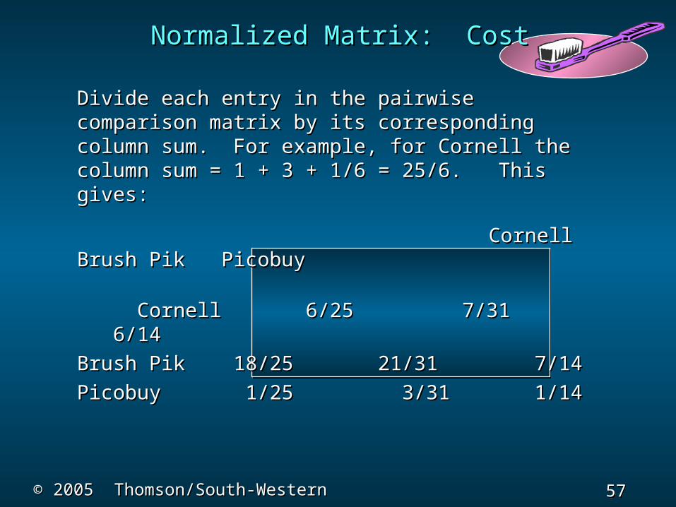
Divide each entry in the pairwise Divide each entry in the pairwise comparison matrix by its corresponding column comparison matrix by its corresponding column sum. For example, for Cornell the column sum = sum. For example, for Cornell the column sum = 1 + 3 + 1/6 = 25/6. This gives:1 + 3 + 1/6 = 25/6. This gives:
Cornell Brush Pik PicobuyCornell Brush Pik Picobuy
CornellCornell 6/25 7/31 6/25 7/31 6/14 6/14
Brush PikBrush Pik 18/25 21/31 18/25 21/31 7/14 7/14
PicobuyPicobuy 1/25 3/31 1/25 3/31 1/14 1/14
Normalized Matrix: CostNormalized Matrix: Cost
58 58 Slide
Slide
© 2005 Thomson/South-Western© 2005 Thomson/South-Western
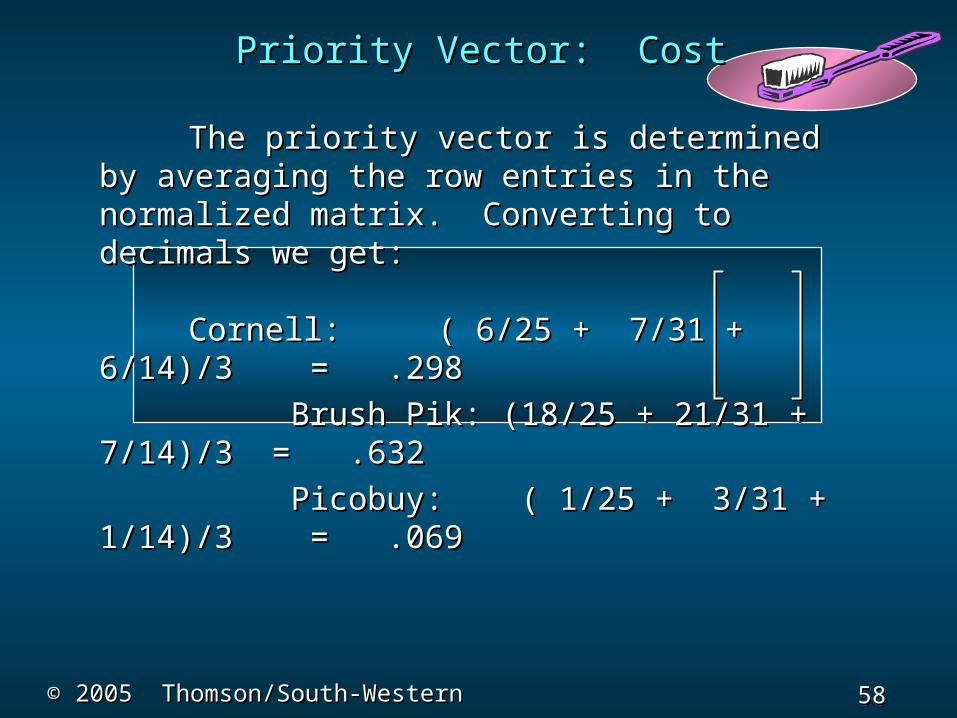
The priority vector is determined by The priority vector is determined by averaging the row entries in the normalized averaging the row entries in the normalized matrix. Converting to decimals we get:matrix. Converting to decimals we get:
Cornell: ( 6/25 + 7/31 + 6/14)/3 Cornell: ( 6/25 + 7/31 + 6/14)/3 = .298 = .298
Brush Pik: (18/25 + 21/31 + 7/14)/3 Brush Pik: (18/25 + 21/31 + 7/14)/3 = .632 = .632
Picobuy: ( 1/25 + 3/31 + 1/14)/3 Picobuy: ( 1/25 + 3/31 + 1/14)/3 = .069 = .069
Priority Vector: CostPriority Vector: Cost
59 59 Slide
Slide
© 2005 Thomson/South-Western© 2005 Thomson/South-Western
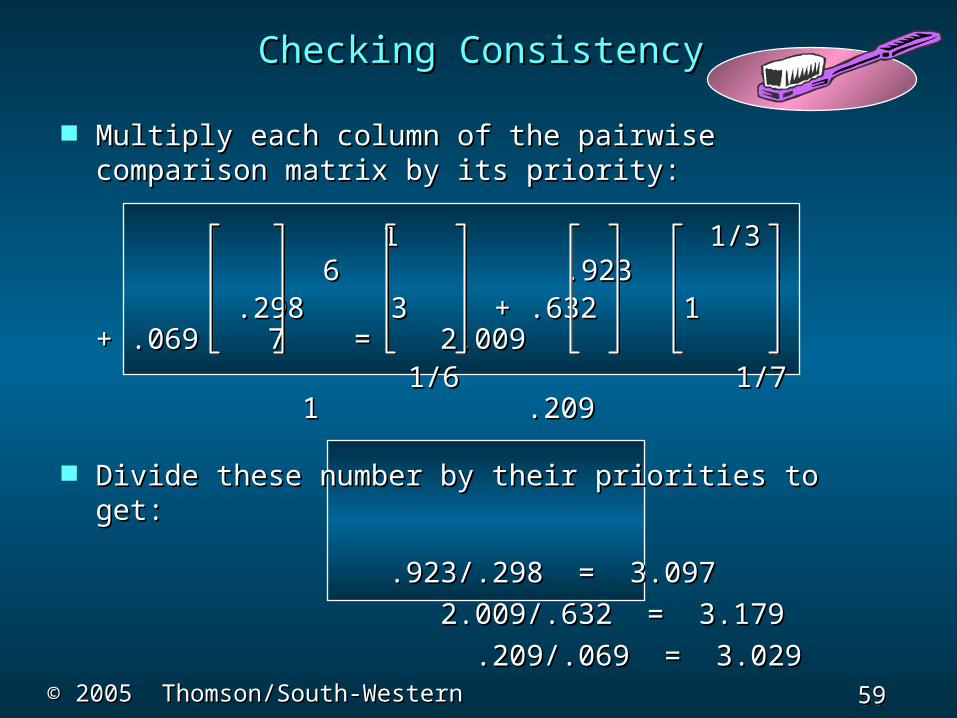
Multiply each column of the pairwise Multiply each column of the pairwise comparison matrix by its priority:comparison matrix by its priority:
1 1/3 1 1/3 6 .923 6 .923
.298 3 + .632 1 + .069 7 = .298 3 + .632 1 + .069 7 = 2.009 2.009
1/6 1/7 1/6 1/7 1 .209 1 .209
Divide these number by their priorities to get:Divide these number by their priorities to get:
.923/.298 = 3.097.923/.298 = 3.097
2.009/.632 = 3.1792.009/.632 = 3.179
.209/.069 = 3.029.209/.069 = 3.029
Checking ConsistencyChecking Consistency
60 60 Slide
Slide
© 2005 Thomson/South-Western© 2005 Thomson/South-Western
Average the above results to get Average the above results to get maxmax..
maxmax = (3.097 + 3.179 + 3.029)/3 = 3.102 = (3.097 + 3.179 + 3.029)/3 = 3.102
Compute the consistence index, CI, for two terms.Compute the consistence index, CI, for two terms.
CI = (CI = (maxmax - - nn)/()/(nn - 1) = (3.102 - 3)/2 - 1) = (3.102 - 3)/2 = .051= .051
Compute the consistency ratio, CR, by CI/RI, Compute the consistency ratio, CR, by CI/RI, where RI = .58 for 3 factors:where RI = .58 for 3 factors:
CR = CI/RI = .051/.58 = .088CR = CI/RI = .051/.58 = .088
Since the consistency ratio, CR, is less than .10, Since the consistency ratio, CR, is less than .10, this is well within the acceptable range for this is well within the acceptable range for consistency. consistency.
Checking ConsistencyChecking Consistency

61 61 Slide
Slide
© 2005 Thomson/South-Western© 2005 Thomson/South-Western
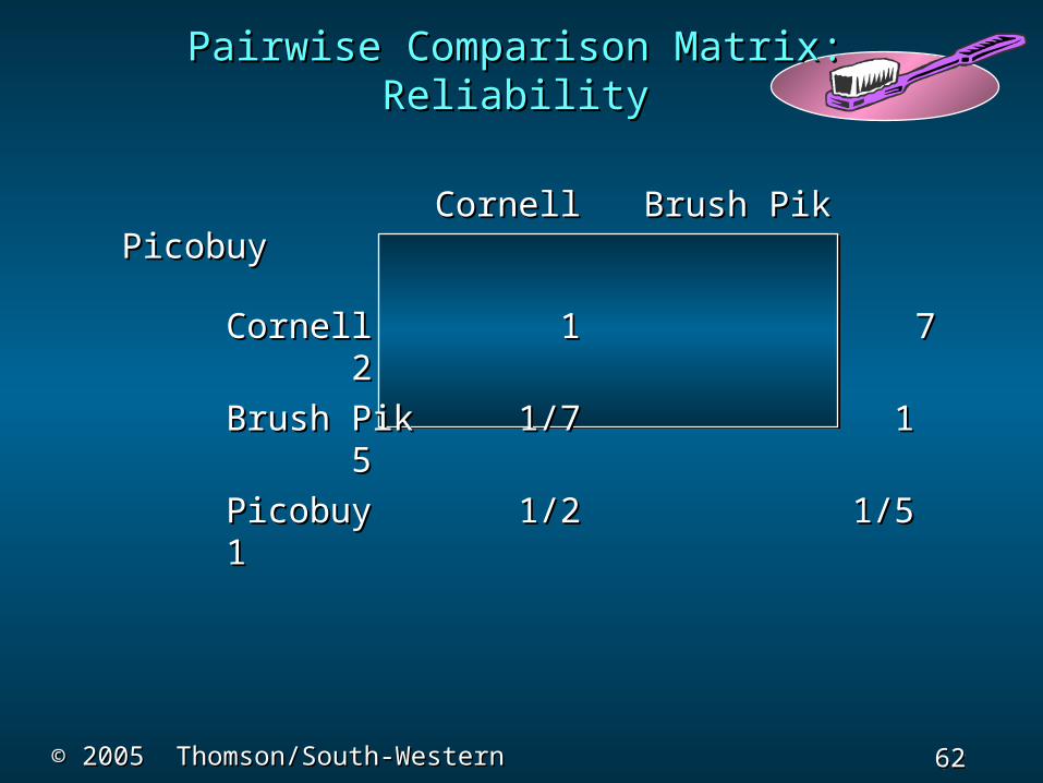
Gill Glass has determined that for Gill Glass has determined that for reliabilityreliability,,
Cornell is very strongly preferable to Brush Pik Cornell is very strongly preferable to Brush Pik andand
equally preferable to Picobuy. Also, Picobuy isequally preferable to Picobuy. Also, Picobuy is
strongly preferable to Brush Pik.strongly preferable to Brush Pik.
Pairwise Comparison Matrix:Pairwise Comparison Matrix:ReliabilityReliability
62 62 Slide
Slide
© 2005 Thomson/South-Western© 2005 Thomson/South-Western
Cornell Brush Pik PicobuyCornell Brush Pik Picobuy
CornellCornell 1 7 1 7 2 2
Brush PikBrush Pik 1/7 1/7 1 1 5 5
PicobuyPicobuy 1/2 1/2 1/5 1/5 1 1
Pairwise Comparison Matrix:Pairwise Comparison Matrix:ReliabilityReliability
63 63 Slide
Slide
© 2005 Thomson/South-Western© 2005 Thomson/South-Western
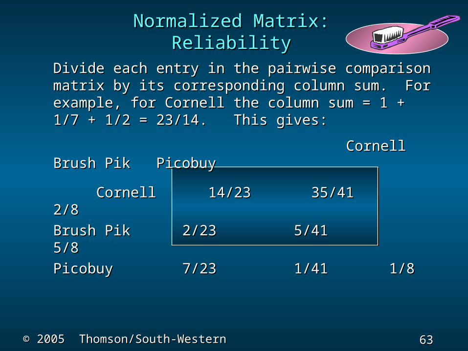
Divide each entry in the pairwise Divide each entry in the pairwise comparison matrix by its corresponding column comparison matrix by its corresponding column sum. For example, for Cornell the column sum sum. For example, for Cornell the column sum = 1 + 1/7 + 1/2 = 23/14. This gives:= 1 + 1/7 + 1/2 = 23/14. This gives:
Cornell Brush Pik Cornell Brush Pik PicobuyPicobuy
CornellCornell 14/23 35/41 14/23 35/41 2/8 2/8
Brush PikBrush Pik 2/23 5/41 2/23 5/41 5/8 5/8
PicobuyPicobuy 7/23 1/41 7/23 1/41 1/8 1/8
Normalized Matrix:Normalized Matrix:ReliabilityReliability
64 64 Slide
Slide
© 2005 Thomson/South-Western© 2005 Thomson/South-Western
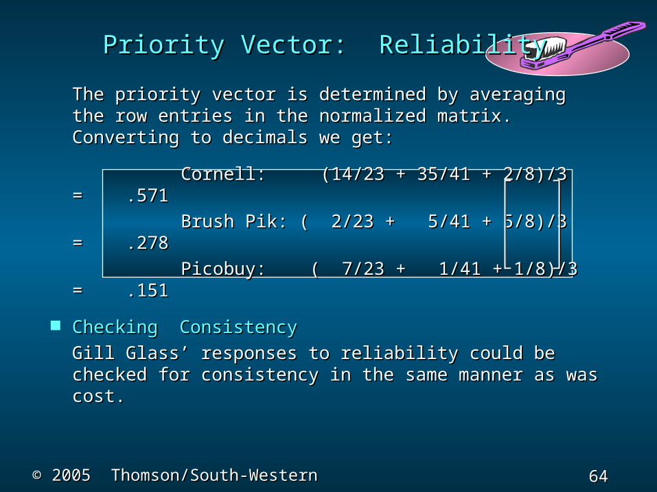
The priority vector is determined by averaging The priority vector is determined by averaging the row entries in the normalized matrix. Converting the row entries in the normalized matrix. Converting to decimals we get:to decimals we get:
Cornell: (14/23 + 35/41 + 2/8)/3 = .571 Cornell: (14/23 + 35/41 + 2/8)/3 = .571
Brush Pik: ( 2/23 + 5/41 + 5/8)/3 = .278 Brush Pik: ( 2/23 + 5/41 + 5/8)/3 = .278
Picobuy: ( 7/23 + 1/41 + 1/8)/3 = .151 Picobuy: ( 7/23 + 1/41 + 1/8)/3 = .151
Checking ConsistencyChecking Consistency
Gill Glass’ responses to reliability could be Gill Glass’ responses to reliability could be checked for consistency in the same manner as was checked for consistency in the same manner as was cost.cost.
Priority Vector: ReliabilityPriority Vector: Reliability
65 65 Slide
Slide
© 2005 Thomson/South-Western© 2005 Thomson/South-Western
Gill Glass has determined that for Gill Glass has determined that for delivery timedelivery time, Cornell is equally preferable to , Cornell is equally preferable to Picobuy. Both Cornell and Picobuy are very Picobuy. Both Cornell and Picobuy are very strongly to extremely preferable to Brush Pik.strongly to extremely preferable to Brush Pik.
Pairwise Comparison Matrix:Pairwise Comparison Matrix:Delivery TimeDelivery Time
66 66 Slide
Slide
© 2005 Thomson/South-Western© 2005 Thomson/South-Western
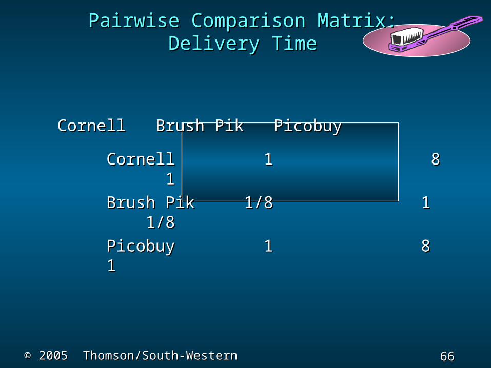
Cornell Brush Pik Cornell Brush Pik PicobuyPicobuy
CornellCornell 1 8 1 8 1 1
Brush PikBrush Pik 1/8 1/8 1 1 1/8 1/8
PicobuyPicobuy 1 1 8 8 1 1
Pairwise Comparison Matrix:Pairwise Comparison Matrix:Delivery TimeDelivery Time
67 67 Slide
Slide
© 2005 Thomson/South-Western© 2005 Thomson/South-Western
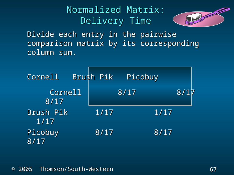
Divide each entry in the pairwise Divide each entry in the pairwise comparison matrix by its corresponding column comparison matrix by its corresponding column sum. sum.
Cornell Brush Pik Cornell Brush Pik PicobuyPicobuy
CornellCornell 8/17 8/17 8/17 8/17 8/178/17
Brush PikBrush Pik 1/17 1/17 1/17 1/17 1/171/17
PicobuyPicobuy 8/17 8/17 8/17 8/17 8/17 8/17
Normalized Matrix:Normalized Matrix:Delivery TimeDelivery Time
68 68 Slide
Slide
© 2005 Thomson/South-Western© 2005 Thomson/South-Western
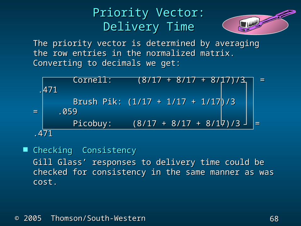
The priority vector is determined by The priority vector is determined by averaging the row entries in the normalized averaging the row entries in the normalized matrix. Converting to decimals we get:matrix. Converting to decimals we get:
Cornell: (8/17 + 8/17 + 8/17)/3 = .471 Cornell: (8/17 + 8/17 + 8/17)/3 = .471
Brush Pik: (1/17 + 1/17 + 1/17)/3 = .059 Brush Pik: (1/17 + 1/17 + 1/17)/3 = .059
Picobuy: (8/17 + 8/17 + 8/17)/3 = .471 Picobuy: (8/17 + 8/17 + 8/17)/3 = .471
Checking ConsistencyChecking Consistency
Gill Glass’ responses to delivery time Gill Glass’ responses to delivery time could be checked for consistency in the same could be checked for consistency in the same manner as was cost.manner as was cost.
Priority Vector:Priority Vector:Delivery TimeDelivery Time
69 69 Slide
Slide
© 2005 Thomson/South-Western© 2005 Thomson/South-Western
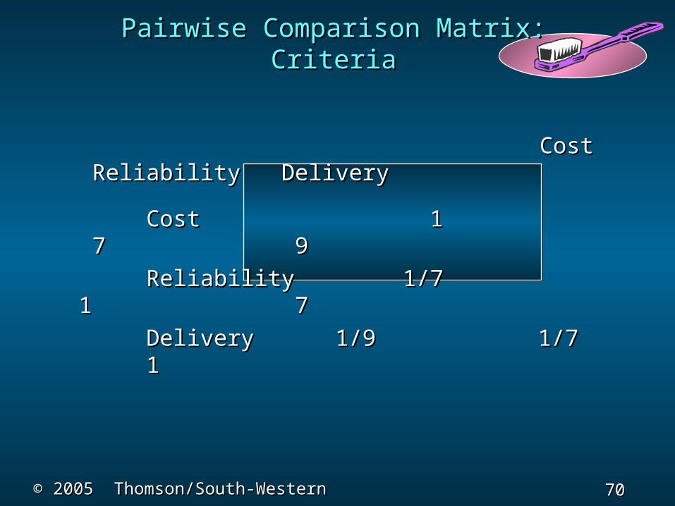
The accounting department has The accounting department has determined that in terms of determined that in terms of criteriacriteria, cost is , cost is extremely preferable to delivery time and very extremely preferable to delivery time and very strongly preferable to reliability, and that strongly preferable to reliability, and that reliability is very strongly preferable to delivery reliability is very strongly preferable to delivery time.time.
Pairwise Comparison Matrix:Pairwise Comparison Matrix:CriteriaCriteria
70 70 Slide
Slide
© 2005 Thomson/South-Western© 2005 Thomson/South-Western
Cost Reliability DeliveryCost Reliability Delivery
CostCost 1 7 1 7 9 9
ReliabilityReliability 1/7 1/7 1 1 7 7
DeliveryDelivery 1/9 1/9 1/7 1/7 1 1
Pairwise Comparison Matrix:Pairwise Comparison Matrix:CriteriaCriteria
71 71 Slide
Slide
© 2005 Thomson/South-Western© 2005 Thomson/South-Western
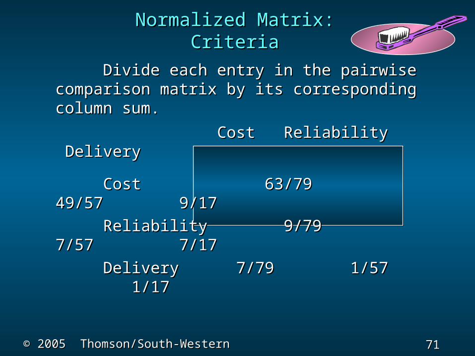
Divide each entry in the pairwise Divide each entry in the pairwise comparison matrix by its corresponding column comparison matrix by its corresponding column sum.sum.
Cost Reliability Cost Reliability DeliveryDelivery
CostCost 63/79 49/57 63/79 49/57 9/179/17
ReliabilityReliability 9/79 7/57 9/79 7/57 7/177/17
DeliveryDelivery 7/79 1/57 7/79 1/57 1/17 1/17
Normalized Matrix:Normalized Matrix:CriteriaCriteria
72 72 Slide
Slide
© 2005 Thomson/South-Western© 2005 Thomson/South-Western
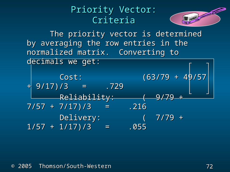
The priority vector is determined by The priority vector is determined by averaging the row entries in the normalized averaging the row entries in the normalized matrix. Converting to decimals we get:matrix. Converting to decimals we get:
Cost: Cost: (63/79 + 49/57 + 9/17)/3 = (63/79 + 49/57 + 9/17)/3 = .729 .729
Reliability: Reliability: ( 9/79 + 7/57 + 7/17)/3 = ( 9/79 + 7/57 + 7/17)/3 = .216 .216
Delivery: Delivery: ( 7/79 + 1/57 + 1/17)/3 = ( 7/79 + 1/57 + 1/17)/3 = .055 .055
Priority Vector:Priority Vector:CriteriaCriteria
73 73 Slide
Slide
© 2005 Thomson/South-Western© 2005 Thomson/South-Western
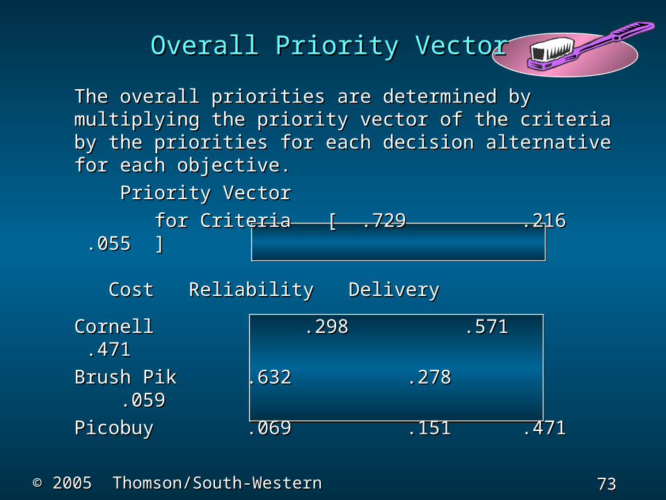
The overall priorities are determined by The overall priorities are determined by multiplying the priority vector of the criteria by multiplying the priority vector of the criteria by the priorities for each decision alternative for the priorities for each decision alternative for each objective.each objective.
Priority VectorPriority Vector
for Criteriafor Criteria [ .729 .216 [ .729 .216 .055 .055 ] ]
Cost Reliability DeliveryCost Reliability Delivery
Cornell Cornell .298 .571 .298 .571 .471 .471
Brush PikBrush Pik .632 .278 .632 .278 .059 .059
PicobuyPicobuy .069 .151 .069 .151 .471 .471
Overall Priority VectorOverall Priority Vector

74 74 Slide
Slide
© 2005 Thomson/South-Western© 2005 Thomson/South-Western
Thus, the overall priority vector is:Thus, the overall priority vector is:
Cornell: (.729)(.298) + (.216)(.571) + (.055)Cornell: (.729)(.298) + (.216)(.571) + (.055)(.471) = .366(.471) = .366
Brush Pik: (.729)(.632) + (.216)(.278) + (.055)Brush Pik: (.729)(.632) + (.216)(.278) + (.055)(.059) = .524(.059) = .524
Picobuy: (.729)(.069) + (.216)(.151) + (.055)Picobuy: (.729)(.069) + (.216)(.151) + (.055)(.471) = .109(.471) = .109
Brush Pik appears to be the overall Brush Pik appears to be the overall recommendation.recommendation.
Overall Priority VectorOverall Priority Vector