07 - inventory management iv - safety stock

Inventory Management IVSafety Stock

Caplice

Lecture 7ESD.260 Fall 2003

© Chris Caplice, MIT2MIT Center for Transportation & Logistics – ESD.260

Assumptions: Basic EOQ ModelDemand

Constant vs VariableKnown vs RandomContinuous vs Discrete

Lead timeInstantaneous Constant or Variable (deterministic/stochastic)

Dependence of itemsIndependentCorrelatedIndentured

Review TimeContinuous vs Periodic

Number of EchelonsOne vs Many

Capacity / ResourcesUnlimited vs Limited

DiscountsNoneAll Units or Incremental

Excess DemandNoneAll orders are backorderedAll orders are lostSubstitution

PerishabilityNoneUniform with time

Planning HorizonSingle PeriodFinite PeriodInfinite

Number of ItemsOneMany


Fundamental Purpose of Inventory

To buffer uncertainties in:- supply,- demand, and/or- transportation

the firm carries safety stocks.

To capture scale economies in:- purchasing,- production, and/or- transportation

the firm carries cycle stocks.


Cycle Stock and Safety Stock

CycleStock

CycleStock

CycleStock

Safety Stock

Time

On Hand

What should my inventory policy be? (how much to order when)

What should my safety stock be?What are my relevant costs?


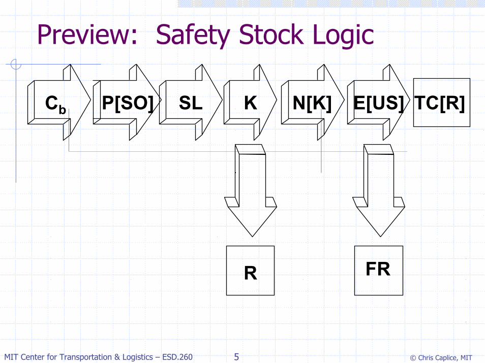
Preview: Safety Stock Logic

P[SO] TC[R]E[US]N[K]

FRR

KSLCb


Determining the Reorder Point

Reorder Point Estimated demand over the lead time (Ft)

Safety Stock

k = SS factorσ = RMSE

R = d' + kσ

( )'R dk

σ−

=

Note1. We usually pick k for desired stock out probability 2. Safety Stock = R – d’


Define Some Terms

Safety Stock Factor (k) Amount of inventory required in terms of

standard deviations worth of forecast error

Stockout Probability = P[d > R]The probability of running out of inventory

during lead time

Service Level = P[d ≤ R] = 1- P[SO]The probability of NOT running out of inventory

during lead time


Service Level and Stockout Probability

Normal Distribution

0.0%0.2%0.4%0.6%0.8%1.0%1.2%1.4%1.6%1.8%

-100 -88

-76

-64

-52

-40

-28

-16 -4 8 20 32 44 56 68 80 92

Demand

Prob

(x)

Reorder Point

Probability of Stockout

Service Level

Where d ~ iid N(d’=10,σ=25)

Forecasted Demand (d’)

SS = kσ


Cumulative Normal Distribution

Cumulative Normal Distribution

0.0%

20.0%

40.0%

60.0%

80.0%

100.0%

120.0%

-100 -86 -72 -58 -44 -30 -16 -2 12 26 40 54 68 82 96

Demand

Prob

(x)

Where d ~ iid N(d’=10,σ=25)

Reorder Point

Probability of Stockout = 1-SL

Service Level


Finding SL from a Given KUsing a Table of Cumulative Normal Probabilities . . .

K 0.00 0.01 0.02 0.03 0.04

0.0 0.5000 0.5040 0.5080 0.5120 0.5160 0.1 0.5398 0.5438 0.5478 0.5517 0.5557 0.2 0.5793 0.5832 0.5871 0.5910 0.5948 0.3 0.6179 0.6217 0.6255 0.6293 0.6331 0.4 0.6554 0.6591 0.6628 0.6664 0.6700 0.5 0.6915 0.6950 0.6985 0.7019 0.7054 0.6 0.7257 0.7291 0.7324 0.7357 0.7389 0.7 0.7580 0.7611 0.7642 0.7673 0.7704 0.8 0.7881 0.7910 0.7939 0.7967 0.7995 0.9 0.8159 0.8186 0.8212 0.8238 0.8264 1.0 0.8413 0.8438 0.8461 0.8485 0.8508

. . . then my Service Level is this value.

If I select a K = 0.42

Or, in Excel, use the function:SL=NORMDIST(kσ+d’, d’, σ, TRUE)


K Factor versus Service Level


Safety Stock and Service Level

Example: if d ~ iid Normal (d’=100,σ=10)What should my SS & R be?

P[SO]

SL

k

Safety Stock

Reorder Point

.50 .50 0 0 100

.10 .90 1.28 13 113

.05 .95 1.65 17 117

.01 .99 2.33 23 123


Service Level

What is exactly is Service Level?

Service Level . . . . IS

IS NOT

Probability that a stockout does not occur during lead time

The fraction of demand satisfied from stock

Probability that stock is available

Fraction of order cycles during which no SO’s occur

Probability that all demand will be satisfied from on hand stock w/in any given replenishment cycle

Fraction of time that stock is available in the system

Fill rate for or availability of an item


So, how do I find Item Fill Rate?

Fill RateFraction of demand met with on-hand inventoryBased on each replenishment cycle

[ ]OrderQuantity E UnitsShortFillRateOrderQuantity

−=

But, how do I find Expected Units Short?More difficultNeed to calculate a partial expectation:


Expected Units Short

( ) [ ][ ]x R

E US x R p x∞

=

= −∑ ( )[ ] ( )o x o oR

E US x R f x dx∞

= −∫

Consider both continuous and discrete casesLooking for expected units short per replenishment cycle.

x

P[x]

1 2 3 4 5 6 7 8

1/8

For normal distribution wehave a nice result:

E[US] = σN[k]Where N[k] = Normal Unit

Loss Function Found in tables or formulaWhat is E[US] if R=5?


The N[k] TableA Table of Unit Normal Loss Integrals

K .00 .01 .02 .03 .04

0.0 .3989 .3940 .3890 .3841 .3793 0.1 .3509 .3464 .3418 .3373 .3328 0.2 .3069 .3027 .2986 .2944 .2904 0.3 .2668 .2630 .2592 .2555 .2518 0.4 .2304 .2270 .2236 .2203 .2169 0.5 .1978 .1947 .1917 .1887 .1857 0.6 .1687 .1659 .1633 .1606 .1580 0.7 .1429 .1405 .1381 .1358 .1334 0.8 .1202 .1181 .1160 .1140 .1120 0.9 .1004 .09860 .09680 .09503 .09328 1.0 .08332 .08174 .08019 .07866 .07716


Item Fill Rate

( )

[ ]

[ ] [ ]1 1

1[ ]

OrderQuantity E UnitsShortFillRate FROrderQuantity

E US N kFRQ QFR Q

N k

σ

σ

−= =

= − = −

−= So, now we can look for

the k that achieves our desired fill rate.


Item Fill Rate ExampleFind fill rate for R=250, 300, 350, and 500 where,

Q = 500 units and demand ~ N(d’=200, σ=100)

R k SL P[SO] N[k] N[k]s FR250 0.5 .69 .31 .1978 19.78 .9604300 1.0 .84 .16 .0833 8.33 .9833350 1.5 .93 .07 .0293 2.93 .9941500 3.0 .999 .001 .0003 .03 .9999

Note:Fill rate is usually much higher than service levelFill rate depends on both R and QQ determines the number of exposures for an item

07 - inventory management iv - safety stock

Documents