03 - chapter03
TRANSCRIPT

Chapter 3Bridge Design Manual - 2002 Load Requirements
Ethiopian Roads Authority Page 3-1
3 LOAD REQUIREMENTS
3.1 SCOPE
This section specifies minimum requirements for loads and forces, the limits of theirapplication, load factors, and load combinations used for the design of new bridges. Theload provisions may also be applied to the structural evaluation of existing bridges.
The design shall be done under the most unfavorable load requirements.
A minimum load factor is specified for force effects that may develop duringconstruction.
This section includes, in addition to traditional loads, the force effects due to collisions,earthquakes, and settlement and distortion of the structure.
Vehicle collisions, earthquakes, and aeroelastic instability develop force effects that aredependent upon structural response. Therefore, such force effects cannot be determinedwithout analysis and/or testing.
With the exception of segmental concrete bridges, construction loads are not provided.
3.2 NOTATIONS
a = length of uniform deceleration at braking (mm)A = seismic acceleration coefficientADTT = average daily truck trafficb = braking force coefficientC = unit cohesion (MPa); coefficient to compute centrifugal forcesCD = drag coefficient (s2 N/mm4)CL = lateral drag coefficientCSm = elastic seismic response coefficient for the mth mode of vibrationDE = minimum depth of earth cover (mm)FSBH = factor of safety against basal heaveg = gravitational acceleration (m/s2)H = final height of retaining wall (mm); notional height of earth pressure diagram
(mm)heq = equivalent height of soil for vehicular load (mm)i = angle of fill to horizontal (°)k = coefficient of earth pressureka = coefficient of active lateral earth pressurekh = coefficient of lateral earth pressureko = coefficient of earth pressure at restkp = coefficient of passive pressureks = coefficient of earth pressure due to surchargem = multiple presence factorOCR = overconsolidation ratiop = pressure of flowing water (MPa); basic earth pressure (MPa); fraction of truck
traffic in a single lane; load intensity (MPa)P = concentrated wheel load (N); live load intensity; load (N)Pa = apparent earth pressure (MPa); force resultant per unit width of wall (N/mm)

Chapter 3Load Requirements Bridge Design Manual - 2002
Page 3-2 Ethiopian Roads Authority
PB = base wind pressure corresponding to a wind speed of 160 km/h (MPa)PD = design wind pressure (MPa)Ph = horizontal component of force per unit length of wall due to earth pressure
(N/mm)PL = lateral water pressure (MPa)PN = normal component of wind pressure (MPa)PP = passive earth pressure (MPa)Pv = vertical component of force per unit length of wall due to earth pressure (N/mm)Q = load intensity (N/mm)q = generalized loadqs = maximum applied surcharge (MPa)R = radius of curvature (mm); seismic response modification factor; radial distance
from point of load application to a point on the wallS = coefficient related to site conditions for use in determining seismic loadsSU = undermined shear strength of cohesive soil (MPa)Tm = period of vibration for mth mode (s)t = thickness of deck (mm)v = highway design speed (m/s); Poisson’s Ratio (DIM)V = design velocity of water (m/s)VB = base wind velocity taken as 160 km/hVDZ = design wind velocity at design Elevation Z (km/h)V0 = friction velocity, a meteorological wind characteristic for various upwind
surface characteristics (km/h)V10 = wind speed at 10 m above low ground or water level (km/h)w = width of clear roadway (mm); width of pier at level of ice action (mm);
density of water (kg/m3)X = horizontal distance from back of wall to point of load application (mm); pier
nose inclination in degreesX1 = distance from the back of the wall to the start of the line load (mm)X2 = length of the live load (mm)Z = structure height above low ground or water level > 10 m; depth below surface of
soil (mm); depth from the ground surface to a point on the wall underconsideration (mm); vertical distance from point of load application to theelevation of a point on the wall under consideration (mm)
Zo = friction length of upstream fetch, a meteorological wind characteristic(m)z = depth below surface of backfill (mm)α = constant for terrain conditions in relation to wind approach; angle between
foundation wall and a line connecting the point on the wall under considerationand a point on the bottom corner of the footing nearest to the wall (RAD)
B = notional slope of backfill (DEG)β = safety index; slope of backfill surface behind retaining wall (DEG)γ = density of materials (kg/m3); density of soil (kg/m3); load factor for limit state
under considerationγs = density of soil (kg/m3)γ's = effective soil density (kg/m3)γEQ = load factor for live load applied simultaneously with seismic loadsγeq = equivalent-fluid density (kg/m3)γi = load factorγP = load factor for permanent loadingγSE = load factor for settlement

Chapter 3Bridge Design Manual - 2002 Load Requirements
Ethiopian Roads Authority Page 3-3
γTG = load factor for temperature gradient∆ = movement of top of wall required reaching minimum active or maximum
passive pressure by tilting or by lateral translation (mm)∆P = constant horizontal earth pressure due to uniform surcharge (MPa)∆ph = horizontal pressure distribution (MPa)δ = friction angle between fill and wall (DEG); angle between foundation wall and a
line connecting the point on the wall under consideration and a point on thebottom corner of the footing furthest from the wall (RAD)
ι = tire contact lengthη = load modifier specified in Chapter 2: General Requirementsθ = angle of wind direction (DEG); angle of backfill of wall to the vertical (DEG);
angle between direction of stream flow and the longitudinal axis of pier (DEG)ϕ = resistance factorsϕf = angle of internal friction of drained soil (DEG)ϕ/ = effective angle of internal friction (DEG)
NOTATIONS ON LOAD AND LOAD DESIGNATION
The following permanent and transient loads and forces shall be considered:
• Permanent LoadsDC = dead load of structural components and nonstructural attachmentsDD = downdragDW = dead load of wearing surfaces and utilitiesEH = horizontal earth pressure loadEL = accumulated locked-in effects resulting from the construction processES = earth surcharge loadEV = vertical pressure from dead load of earth fill
• Transient LoadsBR = vehicular braking forceCE = vehicular centrifugal forceCR = creepCT = vehicular collision forceEQ = earthquakeFR = frictionIM = vehicular dynamic load allowanceLL = vehicular live loadLS = live load surchargePL = pedestrian live loadSE = settlementSH = shrinkageTG = temperature gradientTU = uniform temperatureWA = water load and stream pressureWL = wind on live loadWS = wind load on structure

Chapter 3Load Requirements Bridge Design Manual - 2002
Page 3-4 Ethiopian Roads Authority
3.3 LOAD FACTORS AND COMBINATIONS
GENERAL
The total factored force effect shall be taken as:Q = Σηiγi Qi (3.1)
where:ηi= load modifier (see Chapter 2: General Requirements)Qi = force effects from loads specified hereinγi = load factors specified in Tables 3-2 and 3-3 below
Components and connections of a bridge shall satisfy Equation 3.1 for the applicablecombinations of factored extreme force effects as specified at each of the limit statespresented in Table 3-1:
Table 3-1 Limit States
STRENGTHI
Basic load combination relating to the normal vehicular use of the bridge without wind.
A reduced value of 0.50, applicable to all strength load combinations, specified foruniform temperature (TU), creep (CR), and shrinkage (SH), used when calculating forceeffects other than displacements at the strength limit state, represents an expectedreduction of these force effects in conjunction with the inelastic response of thestructure. The calculation of displacements for these loads utilizes a factor greater than1.0 to avoid undersized joints and bearings.
STRENGTHII
Load combination relating to the use of the bridge by ERA-specified special design orpermit vehicles, without wind.
The permit vehicle should not be assumed to be the only vehicle on the bridge unless soassured by traffic control. Otherwise, the other lanes should be assumed to be occupiedby the vehicular live load as specified herein. For bridges longer than the permitvehicle, the presence of the design lane load, preceding and following the permit load inits lane, should be considered.
STRENGTHIII
Load combination relating to the bridge exposed to wind velocity exceeding 90 km/h.
Vehicles become unstable at higher wind velocities. Therefore, high winds prevent thepresence of significant live load on the bridge.
STRENGTHIV
Load combination relating to very high dead load to live load force effect ratios.
The standard calibration process for the strength limit state consists of trying outvarious combinations of load and resistance factors on a number of bridges and theircomponents. Combinations that yield a safety index close to the target value of β = 3.5are retained for potential application. From these are selected constant load factors γand corresponding resistance factors ϕ for each type of structural component reflectingits use.
This calibration process had been carried out for a large number of bridges with spansnot exceeding 60 m. For the primary components of large bridges, the ratio of dead andlive load force effects is rather high, and could result in a set of resistance factorsdifferent from those found acceptable for small- and medium-span bridges. It isbelieved to be more practical to investigate one additional load case than to require theuse of two sets of resistance factors with the load factors provided in Strength LoadCombination I, depending on other permanent loads present. For bridges with up to180 m spans, Load Combination IV will govern where the dead load to live load forceeffect ratio exceeds 7.0.

Chapter 3Bridge Design Manual - 2002 Load Requirements
Ethiopian Roads Authority Page 3-5
STRENGTHV
Load combination relating to normal vehicular use of the bridge with wind of 90 km/h(25 m/s) velocity
EXTREMEEVENT I
Load combination including earthquake
This limit state includes water loads, WA. The probability of a major flood and anearthquake occurring at the same time is very small. Therefore, consideration of basingwater loads and scour depths on mean discharges shall be warranted. Live loadcoincident with an earthquake is discussed elsewhere in this chapter.
SERVICE I Load combination relating to the normal operational use of the bridge with a 90 km/h(25 m/s) wind and all loads taken at their nominal values. Also related to deflectioncontrol in buried metal structures, tunnel liner plate, and thermoplastic pipe and tocontrol crack width in reinforced concrete structures. This load combination should alsobe used for the investigation of slope stability.
Compression in prestressed concrete components is investigated using this loadcombination. Service III is used to investigate tensile stresses in prestressed concretecomponents.
SERVICE II Load combination intended to control yielding of steel structures and slip of slipcritical connections due to vehicular live load.
This load combination corresponds to the overload provision for steel structures (as inRef 25), and it is applicable only to steel structures. From the point of view of loadlevel, this combination is approximately halfway between that used for Service I andStrength I Limit States.
SERVICE III Load combination relating only to tension in prestressed concrete structures with theobjective of crack control.
The live load specified in these Specifications reflects, among other things, exclusionweight limits. The statistical significance of the 0.80 factor on live load is that the eventis expected to occur about once a year for bridges with two traffic lanes, less often forbridges with more than two traffic lanes, and about once a day for bridges with a singletraffic lane.
FATIGUE Fatigue and fracture load combination relating to repetitive gravitational vehicular liveload and dynamic responses under a single design truck having a constant axle spacingof 9.0 m between 145 kN axles.
The load factor, applied to a single design truck, reflects a load level found to berepresentative of the truck population with respect to a large number of return cycles ofstresses and to their cumulative effects in steel elements, components, and connections.
The load factors for various loads comprising a design load combination shall be taken asspecified in Table 3-2. All relevant subsets of the load combinations shall beinvestigated. For each load combination, every load that is indicated to be taken intoaccount and that is germane to the component being designed, including all significanteffects due to distortion, shall be multiplied by the appropriate load factor and multiplepresence factor specified in Table 3-5, if applicable. The products shall be summed asspecified in Equation 2.1 and multiplied by the load modifiers.
The factors shall be selected to produce the total extreme factored force effect. For eachload combination, both positive and negative extremes shall be investigated.
In load combinations where one force effect decreases another effect, the minimum valueshall be applied to the load reducing the force effect. For permanent force effects, theload factor that produces the more critical combination shall be selected from Table 3-3.

Chapter 3Load Requirements Bridge Design Manual - 2002
Page 3-6 Ethiopian Roads Authority
Where the permanent load increases the stability or load-carrying capacity of acomponent or bridge, the minimum value of the load factor for that permanent load shallalso be investigated.
The larger of the two values provided for load factors of Uniform Temperature (TU),Creep (CR), and Shrinkage (SH) shall be used for deformations and the smaller valuesfor all other effects.
Use one ofthese at a
time
LoadCombination
Limit State
DCDDDWEHEVES
LLIMCEBRPLLSEL
WA WS WL FR TUCRSH
TG SE
EQ CTSTRENGTH 1(Unless noted)
γp 1.75 1.00 - - 1.00 0.50/1.20 γTG γSE - -
STRENGTH II γp 1.35 1.00 - - 1.00 0.50/1.20 γTG γSE - -STRENGTH III γp - 1.00 1.40 - 1.00 0.50/1.20 γTG γSE - -STRENGTH IVEH, EV, ES, DWDC ONLY
γp
1.5- 1.00 - - 1.00 0.50/1.20
- -- -
STRENGTH V γp 1.35 1.00 0.50 1.0 1.00 0.50/1.20 γTG γSE - -EXTREMEEVENT I
γp γEQ 1.00 - - 1.00 - - - 1.00
-
SERVICE I 1.00 1.00 1.00 0.30 1.0 1.00 1.00/1.20 γTG γSE - -SERVICE II 1.00 1.30 1.00 - - 1.00 1.00/1.20 - - - -SERVICE III 1.00 0.80 1.00 - - 1.00 1.00/1.20 γTG γSE - -FATIGUELL, IM and CEONLY
- 0.75 - - - - - - - - -
Ref (24)Where (see following text):
BR = vehicular braking forceCE = vehicular centrifugal forceCR = creepCT = vehicular collision forceDC = dead load of structural componentsDD = downdragDW = dead load of wearing surfaces and utilitiesEH = horizontal earth pressure loadEL = accumulated locked-in effects resulting
from the construction processEQ = earthquake loadES = earth surcharge loadEV = vertical pressure from dead load of earth fill
FR = frictionIM = vehicular dynamic load allowanceLL = vehicular live loadLS = live load surchargePL = pedestrian live loadSE = settlementSH = shrinkageTG = temperature gradientTU = uniform temperatureWA = water load and stream pressureWL = wind on live loadWS = wind load on structure
Table 3-2 - Load Combinations and Load Factors

Chapter 3Bridge Design Manual - 2002 Load Requirements
Ethiopian Roads Authority Page 3-7
Load Factor (γp)Type of LoadMaximum Minimum
DC: Component and Attachments 1.25 0.90DD: Downdrag 1.80 0.45DW: Wearing Surfaces and Utilities 1.50 0.65EH: Horizontal Earth Pressure• Active• At-Rest
1.501.35
0.900.90
EL: Locked-in Erection Stresses 1.0 1.0EV: Vertical Earth Pressure• Overall Stability• Retaining Structure• Rigid Buried Structure• Rigid Frames• Flexible Buried Structures other than
Metal Box Culvert• Flexible Metal Box Culverts
1.351.351.301.351.95
1.50
N/A1.000.900.900.90
0.90
ES: Earth Surcharge 1.50 0.75Ref (24)
Table 3-3 Load Factors for Permanent Loads, γp
The evaluation of overall stability of earth slopes with or without a foundation unitshould be investigated at the service limit state based on the Service I Load Combinationand an appropriate resistance factor. In lieu of better information, the resistance factor,ϕ, shall be taken as:
• When the geotechnical parameters are well defined, and the slope does not support orcontain a structural element.. .............................................................................ϕ = 0.85
• When the geotechnical parameters are based on limited information, or the slopecontains or supports a structural element ......................................................... ϕ = 0.65
For structural (steel) plate box structures with a depth of soil layer of 0.4 - 1.5 m, the liveload factor for the vehicular live loads (LL) and dynamic allowance (IM) shall be takenas 2.0.
This chapter reinforces the traditional method of selecting load combinations to obtainrealistic extreme effects and is intended to clarify the issue of the variability of permanentloads and their effects. The Designer may determine that not all of the loads in a givenload combination apply to the situation under investigation. It is recognized herein thatthe actual magnitude of permanent loads may also be less than the nominal value. Thisbecomes important where the permanent load reduces the effects of transient loads.
In the application of permanent loads, force effects for each of the specified six loadtypes should be computed separately. It is unnecessary to assume that one type of loadvaries by span, length, or component within a bridge. For example, when investigatinguplift at a bearing in a continuous beam, it would not be appropriate to use the maximumload factor for permanent loads in spans that produce a negative reaction, and the

Chapter 3Load Requirements Bridge Design Manual - 2002
Page 3-8 Ethiopian Roads Authority
minimum load factor in spans that produce a positive reaction. Consider the investigationof uplift. Where a permanent load produces uplift, that load would be multiplied by themaximum load factor, regardless of the span in which it is located. If another permanentload reduces the uplift, it would be multiplied by the minimum load factor, regardless ofthe span in which it is located. For example, at Strength I Limit State where thepermanent load reaction is positive and live load can cause a negative reaction, the loadcombination would be:
0.9DC + 0.65DW + 1.75(LL+IM)If both reactions were negative, the load combination would be:
1.25DC + 1.50DW + 1.75(LL+IM).
For each force effect, both extreme combinations may need to be investigated byapplying either the high or the low load factor as appropriate. The algebraic sums of theseproducts are the total force effects for which the bridge and its components should bedesigned.
Water load and friction are included in all strength load combinations at their respectivenominal values.For creep and shrinkage, the specified nominal values should be used. For friction,settlement, and water loads, both minimum and maximum values need to be investigatedto produce extreme load combinations.
The load factor for temperature gradient should be determined on the basis of the:• Type of structure and• Limit state being investigated.Open girder construction and multiple steel box girders have traditionally, but perhapsnot necessarily correctly, been designed without consideration of temperature gradient,i.e., γTG = 0.0.
The load factor for temperature gradient, γTG, and settlement, γSE, should be consideredon a project specific basis. In lieu of project-specific information to the contrary, γTG
shall be taken as:• 0.0 at the strength and extreme event limit states,• 1.0 at the service limit state when live load is not considered, and• 0.50 at the service limit state when live load is considered.
For segmentally constructed bridges, the following load combination shall beinvestigated at the service limit state:
DC+ DW+ EH + EV+ ES+WA+ CR+SH + TG + EL (3.2)
The load factor for live load in Extreme Event Load Combination I, γEQ, shall bedetermined on a project specific basis.
Application of Turkstra's rule for combining uncorrelated loads indicates that γEQ = 0.50is reasonable for a wide range of values of average daily truck traffic (ADTT).
A load factor for passive earth pressure is not given in Table 3-3 because, strictlyspeaking, passive earth pressure is a resistance and not a load.

Chapter 3Bridge Design Manual - 2002 Load Requirements
Ethiopian Roads Authority Page 3-9
3.4 LOAD FACTORS FOR CONSTRUCTION LOADS
Load factors for the weight of the structure and appurtenances shall not be taken to beless than 1.25.
Unless otherwise specified by ERA, the load factor for construction loads, for equipmentand for dynamic effects shall not be less than 1.5. The load factor for wind shall not beless than 1.25. All other load factors shall be taken as 1.0.
The load factors presented here should not relieve the contractor of responsibility forsafety and damage control during construction.
3.5 LOAD FACTORS FOR JACKING AND POSTTENSIONING FORCES
3.5.1 JACKING FORCES
Unless otherwise specified by ERA, the design forces for jacking in service shall not beless than 1.3 times the permanent load reaction at the bearing, adjacent to the point ofjacking. The point of jacking shall be assumed to be 0.5 m from the center of the bearing,if nothing else is stated on the drawing. A minimum height and width of 450 mm shall beprovided for jacking.
Where the bridge will not be closed to traffic during the jacking operation, the jackingload shall also contain a live load reaction consistent with the maintenance of traffic plan,multiplied by the load factor for live load. This special case shall be stated at thepreliminary and detailed drawings or in the Preliminary Design Specifications (PDS).
3.5.2 FORCE FOR POSTTENSIONING ANCHORAGE ZONES
The design force for posttensioning anchorage zones shall be taken as 1.2 times themaximum jacking force.
3.6 DEAD LOADS (DC = STRUCTURAL COMPONENT; DW = WEARING SURFACE; EV =VERTICAL EARTHFILL)
Permanent loads consist of dead loads and earth loads. Dead load shall include the weightof all components of the structure, appurtenances and utilities attached thereto, earthcover, wearing surface, future overlays, and planned widening.
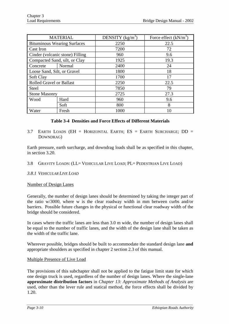
In the absence of more precise information, the densities, specified in Table 3-4, shall beused for dead loads.
The table below provides traditional densities. The density of granular materials dependsupon the degree of compaction and water content. The density of concrete is primarilyaffected by that of the aggregate, which varies by location and design.
Densities shown with the units kg/m3 and kg/mm are in mass units, not force units. Toconvert to force units of N/m3 multiply by the gravitation constant g = 9.81 m/sec2 andcollect the units kgm/sec2 as a Newton, as shown in the table.
Chapter 3Load Requirements Bridge Design Manual - 2002
Page 3-10 Ethiopian Roads Authority
MATERIAL DENSITY (kg/m3) Force effect (kN/m3)Bituminous Wearing Surfaces 2250 22.5Cast Iron 7200 72Cinder (volcanic stone) Filling 960 9.6Compacted Sand, silt, or Clay 1925 19.3Concrete Normal 2400 24Loose Sand, Silt, or Gravel 1800 18Soft Clay 1700 17Rolled Gravel or Ballast 2250 22.5Steel 7850 79Stone Masonry 2725 27.3
Hard 960 9.6WoodSoft 800 8
Water Fresh 1000 10
Table 3-4 Densities and Force Effects of Different Materials
3.7 EARTH LOADS (EH = HORIZONTAL EARTH; ES = EARTH SURCHARGE; DD =DOWNDRAG)
Earth pressure, earth surcharge, and downdrag loads shall be as specified in this chapter,in section 3.20.
3.8 GRAVITY LOADS: (LL= VEHICULAR LIVE LOAD; PL= PEDESTRIAN LIVE LOAD)
3.8.1 VEHICULAR LIVE LOAD
Number of Design Lanes
Generally, the number of design lanes should be determined by taking the integer part ofthe ratio w/3000, where w is the clear roadway width in mm between curbs and/orbarriers. Possible future changes in the physical or functional clear roadway width of thebridge should be considered.
In cases where the traffic lanes are less than 3.0 m wide, the number of design lanes shallbe equal to the number of traffic lanes, and the width of the design lane shall be taken asthe width of the traffic lane.
Wherever possible, bridges should be built to accommodate the standard design lane andappropriate shoulders as specified in chapter 2 section 2.3 of this manual.
Multiple Presence of Live Load
The provisions of this subchapter shall not be applied to the fatigue limit state for whichone design truck is used, regardless of the number of design lanes. Where the single-laneapproximate distribution factors in Chapter 13: Approximate Methods of Analysis areused, other than the lever rule and statical method, the force effects shall be divided by1.20.

Chapter 3Bridge Design Manual - 2002 Load Requirements
Ethiopian Roads Authority Page 3-11
The extreme live load force effect shall be determined by considering each possiblecombination of number of loaded lanes multiplied by the corresponding factor specifiedin Table 3-5. For the purpose of determining the number of lanes when the loadingcondition includes the pedestrian loads specified later in this chapter combined with oneor more lanes of the vehicular live load, the pedestrian loads shall be taken to be oneloaded lane.
The m-factors specified below shall not be applied in conjunction with approximate loaddistribution factors specified in Chapter 13: Approximate Methods of Analysis, exceptwhere the lever rule is used or where special requirements for exterior beams in beam-slab bridges is applied.
Number of Loaded Lanes 1 2 3 >3Multiple Presence Factors
“m”1.20 1.0 0.85 0.65
Table 3-5 Multiple Presence Factors "m"
The multiple presence factors have been included in the approximate equations fordistribution factors in Chapter 13: Approximate Methods of Analysis, both for single andmultiple loaded lanes. The equations are based on evaluation of several combinations ofloaded lanes with their appropriate multiple presence factors and are intended to accountfor the worst case scenario. Where use of the lever rule is specified the Designer mustdetermine the number and location of vehicles and lanes, and, therefore, must include themultiple presence. Stated another way, if a sketch is required to determine loaddistribution, the Designer is responsible for including multiple presence factors andselecting the worst design case. The factor 1.20 from Table 3-5 has already been includedin the approximate equations and should be removed for the purpose of fatigueinvestigations.
The value of m for a single vehicle was estimated at 1.2 on the basis of statisticalcalibration of these Specifications. When a single vehicle is on the bridge, it may beheavier than each one of a pair of vehicles and still have the same probability ofoccurrence.
The consideration of pedestrian loads counting as a "loaded lane" for the purpose ofdetermining a multiple presence factor (m) is based on the assumption that simultaneousoccupancy by a dense loading of people combined with a 75-year design live load isremote. For the purpose of this provision, it has been assumed that if a bridge is used asa viewing stand for eight hours each year for a total time of about one month, theappropriate live load to combine with it would have a one-month recurrence interval.This is reasonably approximated by use of the multiple presence factors, even thoughthey are originally developed for vehicular live loads.
Thus, if a component supported a sidewalk and one lane, it would be investigated for thevehicular live load alone with m = 1.20, and for the pedestrian loads combined with thevehicular live load with m = 1.0. If a component supported a sidewalk and two lanes ofvehicular live load, it would be investigated for:

Chapter 3Load Requirements Bridge Design Manual - 2002
Page 3-12 Ethiopian Roads Authority
• One lane of vehicular live load, m = 1.20;
• The greater of the more significant lane of vehicular live load and the pedestrianloads or two lanes of vehicular live load, m = 1.0 applied to the governing case; and
• Two lanes of vehicular live load and the pedestrian loads, m = 0.85.
The multiple presence factor of 1.20 for a single lane does not apply to the pedestrianloads. Therefore, the case of the pedestrian loads without the vehicular live load is asubset of the second bulleted item.
The multiple presence factors in Table 3-5 were developed based on an ADTT of 5000trucks in one direction. The force effect resulting from the appropriate number of lanesshall be reduced for sites with lower ADTT as follows:
• If 100 ≤ ADTT ≤ 1000; 95 % of the specified force effect shall be used; and
• If ADTT < 100; 90 % of the specified force effect shall be used.
This adjustment is based on the reduced probability of attaining the design event during a75-year design life with reduced truck volume.
3.8.2 DESIGN VEHICULAR LIVE LOAD
Vehicular live loading on the roadways of bridges or incidental structures, designatedHL-93, shall consist of a combination of the:• Design truck or design tandem (see following), and• Design lane load (see following)
Consideration should be given to site-specific modifications to the design truck, designtandem, and/or the design lane load under the following conditions:
• The roadway is expected to carry unusually high percentages of truck traffic;
• Flow control, such as a stop sign, traffic signal, or control booth, causes trucks tocollect on certain areas of a bridge or to not be interrupted by light traffic; or
• Special industrial loads are common due to the location of the bridge.
• See also further discussion in this subchapter.
The live load model, consisting of either a truck or tandem coincident with a uniformlydistributed load, was developed as a notional representation of shear and momentproduced by a group of vehicles routinely permitted on highways under exclusions toweight laws. The vehicles considered to be representative of these exclusions are calledexclusion vehicles. The load model is called "notional" because it is not intended torepresent any particular truck. The exclusion load is the load produced by an exclusionvehicle.
Except as modified in the following subchapter, each design lane under considerationshall be occupied by either the design truck or tandem, coincident with the lane load,where applicable. The loads shall be assumed to occupy 3 m transversely within a designlane.

Chapter 3Bridge Design Manual - 2002 Load Requirements
Ethiopian Roads Authority Page 3-13
The "span" is the length of the simple-span or of one of each of the two continuousspans. The comparison is in the form of ratios of the load effects produced in eithersimple-span or two-span continuous girders. A ratio greater than 1.0 indicates that one ormore of the exclusion vehicles produces a larger load effect than the HS20 loading. Thefigures indicate the degree by which the exclusion loads deviate from the HS loading ofdesignation, e.g., HS25.
The following nomenclature applies to Figures 3-1 through 3-3, which show results oflive load studies involving two equal continuous spans or simple spans:
M POS 0.4L = positive moment at 4/10 point in either spanM NEG 0.4L = negative moment at 4/10 point in either spanM SUPPORT = moment at interior supportVab =shear adjacent to either exterior supportVba = shear adjacent to interior supportMss = midspan moment in a simply supported span
Figures 3-1 shows moment and shear comparisons between the envelope of effectscaused by several truck configurations representative of the exclusion vehicles and theHS20 loading, either the HS20 truck or the lane load, or a load consisting of two 110 kNaxles 1.2 m apart. In the case of negative moment at an interior support, the resultspresented are based on two identical exclusion vehicles in tandem and separated by atleast 15.0 m.
Figure 3-1 Moment and Shear Ratios: Exclusion Vehicles to HS20 (truck or lane)or Two 110 kN Axles at 1.2m

Chapter 3Load Requirements Bridge Design Manual - 2002
Page 3-14 Ethiopian Roads Authority
Figure 3-2 shows comparisons between the force effects produced by a single exclusiontruck per lane and the notional load model, except for negative moment, where thetandem exclusion vehicles were used.
Figure 3-2 Moment and Shear Ratios: Exclusion Vehicles to Notional Model
In the case of negative moment at a support, the provisions of the following subchapterdealing with the application of Design Vehicular Live Loads, requiring investigation of90% of the effect of two design trucks, plus 90 % of the design lane load, have beenincluded in Figure 3-3. Compared with Figure 3-1, the range of ratios can be seen asmore closely grouped:
•Over the span range,•Both for shear and moment, and•Both for simple-span and continuous spans.
The implication of close grouping is that the notional load model with a single-loadfactor has general applicability.
Figure 3-3 shows the ratios of force effects produced by the notional load model and thegreatest of the HS20 truck or lane loading, or Alternate Military Loading.
Figure 3-3 Moment and Shear Ratios: Notional Model to HS20 (truck or lane) orTwo 110 kN Axles at 1.2 m.

Chapter 3Bridge Design Manual - 2002 Load Requirements
Ethiopian Roads Authority Page 3-15
In reviewing Figure 3-3, it should be noted that the total design force effect is also afunction of load factor, load modifier, load distribution, and dynamic load allowance.
3.8.3 DESIGN TRUCK
The weights and spacings of axles and wheels for the design truck shall be as specified inFigure 3-4. A dynamic load allowance shall be considered as specified in the followingsubchapter on Vehicular Dynamic Load Allowance.
Figure 3-4 Characteristics of the Design Truck
Except as specified in following subchapters on the application of Design Vehicular LiveLoads and Fatigue Loads, the spacing between the two 145 kN axles shall be variedbetween 4.3 and 9.0 m to produce extreme force effects.
3.8.4 DESIGN TANDEM
The design tandem used for Strategic Bridges (see Chapter 2: General Requirements)shall consist of a pair of 110 kN axles spaced 1.2 m apart. The transverse spacing ofwheels shall be taken as 1.8 m. A dynamic load allowance shall be considered asspecified in a following subchapter. The spacing and loading is illustrated in Figure 3-5.
3.000 mm
4.3 m
4.3 –9.0 m
1.8 m
Plan of Design Truck Loadshowing tire contact areas

Chapter 3Load Requirements Bridge Design Manual - 2002
Page 3-16 Ethiopian Roads Authority
Figure 3-5 Design Tandem Load
3.8.5 DESIGN LANE LOAD
The design lane load shall consist of a load of 9.3 kN/m, uniformly distributed in thelongitudinal direction. Transversely, the design lane load shall be assumed to beuniformly distributed over a 3.0-m width. The force effects from the design lane loadshall not be subject to a dynamic load allowance.
3.8.6 TIRE CONTACT AREA
The tire contact area of a wheel consisting of one or two tires shall be assumed to be asingle rectangle, whose width is 500 mm and whose length (ι) in mm shall be taken as:
ι = 2.28 x 10⁻³ γ (1 + IM/100) P (3.3)
where: γ = load factor for the limit state under consideration.IM = dynamic load allowance percentP = 72.5 kN for the design truck and 55 kN for the design tandem
The implication of extending the length of the tire patch by the load factor is that thecontact pressure remains nearly constant as load varies.
The tire pressure shall be assumed to be uniformly distributed over the contact area. Thetire pressure shall be assumed to be distributed as follows:• On continuous surfaces, uniformly over the specified contact area, and• On interrupted surfaces, uniformly over the actual contact area within the footprint
with the pressure increased in the ratio of the specified to actual contact areas.
However, for all concrete decks including composite decks the length 200 mm shall beused in Equation 3.3.
3.8.7 DISTRIBUTION OF WHEEL LOADS THROUGH EARTH FILLS
Where the depth of fill is less than 600 mm, the effect of the fill on the distribution oflive load shall be neglected.
Where the depth of fill exceeds 600 mm, wheel loads shall be considered to be uniformlydistributed over a rectangular area with sides equal to the dimension of the tire contactarea, as specified above, and increased by either 1.15 times the depth of the fill in selectgranular backfill, or 1.0 times the depth of the fill in all other cases. The provisions of
110 kN
110 kN
1.2 m
1.8 m
Chapter 3Bridge Design Manual - 2002 Load Requirements
Ethiopian Roads Authority Page 3-17
the present sub section on Multiple Presence of Live Load, and Application of DesignVehicular Live Loads (sub-section n°3.9) shall apply.
Where such areas from several wheels overlap, the total load shall be uniformlydistributed over the area.
For single-span culverts, the effects of live load shall be neglected where the depth offill is more than 2.4 m and exceeds the span length; for multiple span culverts, the effectsshall be neglected where the depth of fill exceeds the distance between faces of endwalls.
Where the live load and impact moment in concrete slabs, based on the distribution of thewheel load through earth fills, exceeds the live load and impact moment calculatedaccording to Chapter 13: Approximate Methods of Analysis, Section 13.5: EquivalentStrip Widths for Slab-type Bridges, or a more refined method, the latter moment shall beused.
This approximation is similar to the 60° rule found in many texts on soil mechanics.
This provision applies to relieving slabs below grade and to top slabs of box culverts.
3.9 APPLICATION OF DESIGN VEHICULAR LIVE LOADS
3.9.1 GENERAL
The effects of an axle sequence and the lane load are superimposed in order to obtainextreme values.
Unless otherwise specified, the extreme force effect shall be taken as the larger of thefollowing:• The effect of the design tandem combined with the effect of the design lane load, or• The effect of one design truck with the variable axle spacing specified in the
subchapter Multiple Presence of Live Load above, combined with the effect of thedesign lane load, and
• For both negative moment between points of contraflexure under a uniform load onall spans, and reaction at interior piers only, 90% of the effect of two design trucksspaced a minimum of 15.0 m between the lead axle of one truck and the rear axle ofthe other truck, combined with 90% of the effect of the design lane load. The distancebetween the 145 kN axles of each truck shall be taken as 4.3 m.
Axles that do not contribute to the extreme force effect under consideration shall beneglected.
Both the design lanes and the 3m loaded width in each lane shall be positioned toproduce extreme force effects. The design truck or tandem shall be positionedtransversely such that the center of any wheel load is not closer than:
• For the design of the deck overhang - 300 mm from the face of the curb or railing,and
• For the design of all other components - 600 mm from the edge of the design lane.

Chapter 3Load Requirements Bridge Design Manual - 2002
Page 3-18 Ethiopian Roads Authority
Unless otherwise specified, the lengths of design lanes, or parts thereof, that contribute tothe extreme force effect under consideration, shall be loaded with the design lane load.
The lane load is not interrupted to provide space for the axle sequences of the designtandem or the design truck; interruption is needed only for patch loading patterns toproduce extreme force effects.
The notional design loads were based on the information described in the abovesubchapter Design Vehicular Live Load, which contained data on vehicles weighing up toabout 490 kN. Where multiple lanes of heavier versions of this type of vehicle areconsidered probable, consideration should be given to investigating negative moment andreactions at interior supports for pairs of the design tandem spaced from 8 m to 12 mapart, combined with the design lane load specified in subchapter Design Lane Loadabove. This is consistent with above subchapter Design Vehicular Live Load, and shouldnot be considered a replacement for the Strength II Load Combination.
Only those areas or parts of areas that contribute to the same extreme being soughtshould be loaded. The loaded length should be determined by the points where theinfluence surface meets the centerline of the design lane.
Where a sidewalk is not separated from the roadway by a crashworthy traffic barrier,consideration should be given to the possibility that vehicles can climb up the sidewalk.
3.9.2 LOADING FOR OPTIONAL LIVE LOAD DEFLECTION EVALUATION
The criteria for live load deflection shall be considered optional. These provisions permitbut do not encourage its use. If the owner chooses to invoke deflection control, thedeflection should be taken as the larger of:• That resulting from the design truck alone, or• That resulting from 25 % of the design truck taken together with the design lane load
In deflection control, the following principles shall apply:• When investigating the maximum absolute deflection, all design lanes should be
loaded, and all supporting components should be assumed to deflect equally• When investigating maximum relative displacements, the number and position of
loaded lanes shall be selected to provide the worst differential effect• The live load portion of Load Combination Service I shall be used, including the
dynamic load allowance, IM
Note that live load deflection is a service issue, not a strength issue. Experience withbridges designed under previous Specifications indicated no adverse effects of live loaddeflection. Therefore, there appears to be little reason to require that the past criteria becompared to a deflection based upon the heavier live load required by theseSpecifications.
The provisions of this subsection are intended to produce apparent live load deflectionssimilar to those used in the past. The current design truck is identical to the HS-20 truckof past Standard Specifications. For the span lengths where the design lane load controls,the design lane load together with 25% of the design truck, i.e., three concentrated loadstotaling 80 kN, is similar to the past lane load with its single concentrated load of 80 kN.

Chapter 3Bridge Design Manual - 2002 Load Requirements
Ethiopian Roads Authority Page 3-19
3.9.3 DESIGN LOADS FOR DECKS, DECK SYSTEMS, AND THE TOP SLABS OF BOX CULVERTS
This subchapter clarifies the selection of wheel loads to be used in the design of bridgedecks, slab bridges, and top slabs of box culverts.
The design load is always an axle load; single wheel loads should not be considered.
Where the approximate strip method is used to analyze decks and top slabs of boxculverts, force effects shall be determined on the following basis:
• Where primary strips are transverse and their span does not exceed 4.6m, thetransverse strips shall be designed for the wheels of the 145 kN axle.
• Where primary strips are transverse and their span exceeds 4.6m, the transverse stripsshall be designed for the wheels of the 145 kN axle and the lane load.
• Where primary strips are longitudinal, the transverse strips shall be designed for allloads specified in above subchapter Design Vehicular Live Load, including the laneload.
Where the refined methods are used, all of the loads specified in above subchapterDesign Vehicular Live Load, including the lane load, shall be considered.
Deck systems, including slab-type bridges, shall be designed for all of the live loadsspecified in above subchapter Design Vehicular Live Load, including the lane load.
Wheel loads shall be assumed equal within an axle unit, and amplification of the wheelloads due to centrifugal and braking forces need not be considered for the design ofdecks.
It is theoretically possible that an extreme force effect could result from a 145 kN axle inone lane and a 220 kN tandem in a second lane, but such sophistication is not warrantedin practical design.
3.9.4 DECK OVERHANG LOAD
For the design of deck overhangs with a cantilever, not exceeding 1.8 m from thecenterline of the exterior girder to the face of a structurally continuous concrete railing,the outside row of wheel loads shall be replaced with a uniformly distributed line load of15 kN/m intensity, located 0.3 m from the face of the railing.
Structurally continuous barriers and edge-beams have been observed to be effective indistributing wheel loads in the overhang. Implicit in this provision is the assumption thatthe 110 kN half weight of a design tandem is distributed over a longitudinal length of 7.6m, and that there is a cross beam or other appropriate component at the end of the bridgesupporting the barrier which is designed for the half tandem weight. This provision doesnot apply if the barrier is not structurally continuous.
3.10 FATIGUE LOAD
Since the fatigue and fracture limit state is defined in terms of accumulated stress-rangecycles, specification of load alone is not adequate. Load should be specified along withthe frequency of load occurrence.

Chapter 3Load Requirements Bridge Design Manual - 2002
Page 3-20 Ethiopian Roads Authority
For the purposes of this chapter, a truck is defined as any vehicle with more than eithertwo axles or four wheels.
3.10.1 MAGNITUDE AND CONFIGURATION
The fatigue load shall be one design truck or axles thereof specified in above subchapterDesign Truck, but with a constant spacing of 9.0 m between the 145 kN axles. Thedynamic load allowance specified in the following subchapter of that name shall beapplied to the fatigue load.
3.10.2 FREQUENCY
The frequency of the fatigue load shall be taken as the single-lane average daily trucktraffic (ADTTSL). This frequency shall be applied to all components of the bridge, evento those located under lanes that carry a lesser number of trucks.
In the absence of better information, the single-lane ADTT shall be taken as:
ADTTSL = P * ADTT (3.4)where:
ADTT= the number of trucks per day in one direction averaged over the design lifeADTTSL = the number of trucks per day in a single-lane averaged over the design lifeP = taken as specified in Table 3-6 below:
Number of LanesAvailable to Trucks
P
1 1.002 0.85
3 or more 0.80
Table 3-6 Fraction of Truck Traffic in a Single Lane, P
The single-lane ADTT is that for the traffic lane in which the majority of the truck trafficcrosses the bridge. On a typical bridge with no nearby entrance/exit ramps, the shoulderlane carries most of the truck traffic.
Since future traffic patterns on the bridge are uncertain, the frequency of the fatigue loadfor a single lane is assumed to apply to all lanes.
The ADTT can be determined by multiplying the ADT by the fraction of trucks in thetraffic. In lieu of site-specific fraction of truck traffic data, the values of Table 3-7 shallbe applied for routine bridges. The table is based on traffic counts at seven locations inthe country:
Class of Highway Fraction of Trucks in TrafficRural Highway 0.40Urban Highway 0.30Other Rural Roads 0.45Other Urban Roads 0.35
Table 3-7 Fraction of Trucks in Traffic

Chapter 3Bridge Design Manual - 2002 Load Requirements
Ethiopian Roads Authority Page 3-21
3.10.3 LOAD DISTRIBUTION FOR FATIGUE
Refined Methods
• A refined method is any method of analysis that satisfies the requirements ofequilibrium and compatibility and utilizes stress-rain relationships for the proposedmaterials, including, but not limited to:
• Classical force and displacement methods: a method of analysis in which thestructure is divided into components whose stiffness can be independently calculated.Equilibrium and compatibility among the components is restored by determining theinterface forces.
• Finite difference method: a method of analysis in which the governing differentialequation is satisfied at discrete points on the structure.
• Finite element method: a method of analysis in which a structure is discretized intoelements connected at nodes, the shape of the element displacement field is assumed,partial or complete compatibility is maintained among the element interfaces, andnodal displacements are determined by using energy variational principles orequilibrium methods.
• Folded plate method: a method of analysis in which the structure is subdivided intoplate components, and both equilibrium and compatibility requirements are satisfiedat the component surfaces.
• Finite strip method: a method of analysis in which a structure is discretized intoparallel strips. The shape of the strip displacement field is assumed and partialcompatibility is maintained among the element interfaces. Model displacementparameters are determined by using energy variational principles or equilibriummethods.
• Grillage analogy method: a method of analysis in which all or part of thesuperstructure is discretized into orthotropic components that represent thecharacteristics of the structure.
• Series or other harmonic methods: a method of analysis in which the load model issubdivided into suitable parts, allowing each part to correspond to one term of aconvergent infinite series by which structural deformations are described.
• Yield line method: a method of analysis in which a number of possible yield linepatterns are examined in order to determine load-carrying capacity.
The Designer shall be responsible for the implementation of computer programs used tofacilitate structural analysis and for the interpretation and use of results. The choice of theRefined Method will depend on the computer program.
If it were assured that the traffic lanes would remain as they are indicated at the openingof the bridge throughout its entire service life, it would be appropriate to place the truckat the center of the traffic lane that produces maximum stress range in the detail underconsideration. But because future traffic patterns on the bridge are uncertain and in theinterest of minimizing the number of calculations required of the designer, the position ofthe truck is made independent of the location of both the traffic lanes and the designlanes.
Where the bridge is analyzed by any refined method, a single design truck shall bepositioned transversely and longitudinally to maximize stress range at the detail underconsideration, regardless of the position of traffic or design lanes on the deck.

Chapter 3Load Requirements Bridge Design Manual - 2002
Page 3-22 Ethiopian Roads Authority
Approximate Methods (see chapter 13: Approximate Methods of Analysis)
Where the bridge is analyzed by approximate load distribution, the distribution factor forone traffic lane shall be used.
3.11 RAIL TRANSIT LOAD
Where a bridge also carries rail-transit vehicles, the Owner of the Railway shall specifythe transit load characteristics and the expected interaction between transit and highwaytraffic.
If rail transit is designed to occupy an exclusive lane, transit loads should be included inthe design, but the bridge should not have less strength than if it had been designed as ahighway bridge of the same width.
If the rail transit is supposed to mix with regular highway traffic, the Owner shouldspecify or approve an appropriate combination of transit and highway loads for thedesign. Transit load characteristics may include:
• Loads,
• Load distribution,
• Load frequency,
• Dynamic allowance, and
• Dimensional requirements.
3.12 PEDESTRIAN LOADS
A pedestrian load of 4.0 kPa (kN/m2) shall be applied to all sidewalks wider than 0.6 mand considered simultaneously with the vehicular design live load.
See the provisions of above subchapter Multiple Presence of Live Load for applying thepedestrian loads in combination with the vehicular live load. Usually the 4 kN/m2 loadwill allow for small cars to pass. To avoid accidents for bridges wider than 2.4 m,provision shall be make for an additional axle load.
Where sidewalks, pedestrian, and/or bicycle bridges are intended to be used bymaintenance and/or other incidental vehicles, these loads shall be considered in thedesign. If unknown, at least one movable axle load of 70 kN acting together with thepedestrian load shall be applied. The dynamic load allowance need not be considered forthese vehicles.
In half-through-trusses of steel, the compressed top chord of a simple span truss shall bedesigned to resist a lateral force of not less than 4.0 kN/m length, considered as apermanent load for the Strength I Load Combination and factored accordingly.

Chapter 3Bridge Design Manual - 2002 Load Requirements
Ethiopian Roads Authority Page 3-23
3.13 DYNAMIC LOAD ALLOWANCE (IM = VEHICULAR DYNAMIC LOAD ALLOWANCE)
3.13.1 GENERAL
Unless otherwise permitted in subchapters Buried Components and Wood Componentsbelow, the static effects of the design truck or tandem, other than centrifugal and brakingforces, shall be increased by the percentage specified in Table 3-8 for dynamic loadallowance.
The factor to be applied to the static load shall be taken as: (1 + IM/100).
The dynamic load allowance shall not be applied to pedestrian loads or to the design laneload.
Component IMDeck Joints – All Limit States 75%All Other Components• Fatigue and Fracture Limit State• All Other Limit States
15%33%
Table 3-8 Dynamic Load Allowance, IM
Dynamic load allowance need not be applied to:
• Retaining walls not subject to vertical reactions from the superstructure, and• Foundation components that are entirely below ground level.
The dynamic load allowance shall be reduced for components, other than joints, ifjustified by sufficient evidence, but in no case shall the dynamic load allowance used indesign be less than 50% of IM in the table above.
The dynamic load allowance (IM) in Table 3-8 is an increment to be applied to the staticwheel load to account for wheel load impact from moving vehicles.
Dynamic effects due to moving vehicles shall be attributed to two sources:
• Hammering effect is the dynamic response of the wheel assembly to riding surfacediscontinuities, such as deck joints, cracks, potholes, and delaminations, and
• Dynamic response of the bridge as a whole to passing vehicles, which shall be due tolong undulations in the roadway pavement, such as those caused by settlement of fill,or to resonant excitation as a result of similar frequencies of vibration between bridgeand vehicle. The frequency of vibration of any bridge should not exceed 3 Hz.
Field tests indicate that in the majority of highway bridges, the dynamic component ofthe response does not exceed 25% of the static response to vehicles. This is the basis fordynamic load allowance with the exception of deck joints. However, the specified liveload combination of the design truck and lane load, represents a group of exclusionvehicles that are at least 4/3 of those caused by the design truck alone on short andmedium-span bridges. The specified value of 33% in Table 3-8 is the product of 4/3 andthe basic 25%.

Chapter 3Load Requirements Bridge Design Manual - 2002
Page 3-24 Ethiopian Roads Authority
This subchapter recognizes the damping effect of soil when in contact with some buriedstructural components, such as footings. To qualify for relief from impact, the entirecomponent must be buried. For the purpose of this chapter, a retaining type componentis considered to be buried to the top of the fill.
3.13.2 BURIED COMPONENTS
The dynamic load allowance for culverts and other buried structures, in %, shall be takenas:
IM = 33 (1.0 - 4.l*10-4 DE) > 0% (3.5)Where:
DE = the minimum depth of earth cover above the structure (mm)
3.13.3 WOOD COMPONENTS
Wood structures are known to experience reduced dynamic wheel load effects due tointernal friction between the components and the damping characteristics of wood.
For wood bridges and wood components of bridges, the dynamic load allowance valuesspecified in Table 3-8 shall be reduced to 70 % of the values specified therein for IM.
3.14 CENTRIFUGAL FORCES (CE= VEHICULAR CENTRIFUGAL FORCE)
Centrifugal forces shall be taken as the product of the axle weights of the design truck ortandem and the factor C, taken as:
C = 4 v2 (3.6)3 g*R
where: v = highway design speed (m/s)g = gravitational acceleration: 9.81 (m/s2)R = radius of curvature of traffic lane (m)
Highway design speed shall not be taken to be less than the value specified in theGeometric Design Manual-2002, Chapter 5: Design Controls & Criteria, Section 5.8:Design Speed. The multiple presence factors specified above in subchapter MultiplePresence of Live Load shall apply. Centrifugal forces shall be applied horizontally at adistance 1.8 m above the roadway surface.
Lane load is neglected in computing the centrifugal force, as the spacing of vehicles athigh speed is assumed to be large, resulting in a low density of vehicles following and/orpreceding the design truck.
The specified live load combination of the design truck and lane load, however,represents a group of exclusion vehicles that produce force effects of at least 4/3 of thosecaused by the design truck alone on short and medium-span bridges. This ratio isindicated in Equation 3.6. Thus, the provision is not technically perfect, yet it reasonablymodels the representative exclusion vehicle traveling at design speed with largeheadways to other vehicles. The approximation attributed to this convenientrepresentation is acceptable in the framework of the uncertainty of centrifugal force fromrandom traffic patterns.

Chapter 3Bridge Design Manual - 2002 Load Requirements
Ethiopian Roads Authority Page 3-25
3.15 BRAKING FORCE (BR= VEHICULAR BRAKING FORCE)
Based on energy principles, and assuming uniform deceleration (retardation), the brakingforce determined as a fraction "b" of vehicle weight is:
b = v2 (3.7)2ga
wherea = the length of uniform deceleration.
Calculations using a braking length of 122 m and a speed of 90 km/h (25 m/s) yield b =0.26 for a horizontal force that will act for a period of about 10 seconds. The factor "b"applies to all lanes in one direction because all vehicles may have reacted within this timeframe. Only the design truck or tandem are to be considered because other vehicles,represented by the design lane load, are expected to brake out of phase.
Braking forces shall be taken as 25 % of the axle weights of the design truck or tandemper lane placed in all design lanes which are considered to be loaded in accordance withabove subchapter Number of Design Lanes, and which are carrying traffic headed in thesame direction. These forces shall be assumed to act horizontally at the level of theroadway surface in either longitudinal direction to cause extreme force effects. All designlanes shall be simultaneously loaded for bridges likely to become one-directional in thefuture.
The multiple presence factors specified in above subchapter Multiple Presence of LiveLoad shall apply.
3.16 VEHICULAR COLLISION FORCE (CT= VEHICULAR COLLISION FORCE)
3.16.1 PROTECTION OF STRUCTURES
For the purpose of this subchapter, a barrier shall be considered structurally independentif it does not transmit loads to the bridge.
The provisions of this subchapter need not be considered for structures which areprotected by:
• An embankment;• A structurally independent, crashworthy ground mounted 1.4-m high barrier, located
within 3.0 m from the component being protected; or• A 1.1-m high barrier located at more than 3.0 m from the component being protected.• In order to qualify for this exemption, the engineer shall approve that such barrier
shall be structurally and geometrically capable of surviving a vehicular collision.
Full-scale crash tests have shown that some vehicles have a greater tendency to lean overor partially cross over a 1.1-m high barrier than a 1.4-m high barrier. This behaviorwould allow a significant collision of the vehicle with the component being protected ifthe component is located within a meter or so of the barrier. If the component is morethan about 3.0 m behind the barrier, the difference between the two barrier heights is nolonger important.

Chapter 3Load Requirements Bridge Design Manual - 2002
Page 3-26 Ethiopian Roads Authority
3.16.2 VEHICLE AND RAILWAY COLLISION WITH STRUCTURES
Unless protected as specified above, abutments and piers located within a distance of 6.0m to the edge of roadway, or to the centerline of a railway track, shall be designed for anequivalent static force of 1800 kN, which is assumed to act in any direction in ahorizontal plane, at a distance of 1.2 m above ground.
It is not the intent of this provision to encourage unprotected piers and abutments withinthe setbacks indicated, but rather to supply some guidance for structural design when it isdeemed totally impractical to meet the requirements given above.
The equivalent static force of 1800 kN is based on the information from full-scale crashtests of barriers for redirecting 360 kN tractor-trailers and from analysis of other truckcollisions. The 1800 kN train collision load is based on physically unverified analyticalwork. For individual column shafts, the 1800 kN load should be considered a point load.For wall piers, the load shall be considered to be a point load or shall be distributed overan area deemed suitable for the size of the structure and the anticipated impactingvehicle, but not greater than 1.5 m wide by 0.6 m high. These dimensions weredetermined by considering the size of a truck frame
3.16.3 VEHICLE COLLISION WITH BARRIERS
The railing shall be either an ERA Standard Railing (see Standard Detail Drawings-2002, Chapter 2: Guardrail Drawings and Chapter 7: Bridge Drainage, Drawing B-34)or any other railing approved by ERA.
3.17 WATER LOADS (WA= WATER LOAD AND STREAM PRESSURE)
3.17.1 STATIC PRESSURE
Static pressure of water shall be assumed to act perpendicular to the surface that isretaining the water. Pressure shall be calculated as the product of height of water abovethe point of consideration, the density of water, and "g" (the acceleration of gravity =9.81 m/s2).p = γ * g * z * 10-9 (3.8)where p = static pressure (Mpa)
γ = density of water (kg/m3)z = height of water above the point of consideration (mm)g = Gravitational acceleration (m/s2)
Design water levels for various limit states shall be as specified and/or approved by ERA.If nothing else is stated, the assumed water level at the service limit state shall be thedesign level and the strength limit state 20%, or at least 0.2 m, above the design level.
3.17.2 BUOYANCY
Buoyancy shall be considered an uplift force, taken as the sum of the vertical componentsof static pressures, as specified above, acting on all components below design waterlevel.

Chapter 3Bridge Design Manual - 2002 Load Requirements
Ethiopian Roads Authority Page 3-27
For substructures with cavities in which the presence or absence of water cannot beascertained, the condition producing the least favorable force effect should be chosen.
3.17.3 STREAM PRESSURE
Longitudinal
For the purpose of this chapter, the longitudinal direction refers to the major axis of asubstructure unit.
The pressure of flowing water acting in the longitudinal direction of substructures shallbe taken as:
p = 5.14*10-4 CDV2 (3.9)
where: p = pressure of flowing water (MPa)CD = drag coefficient for piers as specified in Table 3-9V = design velocity in m/s of water for the design flood in strength and
service limit states and for the check flood in the extreme event limitstate (see ERA Drainage Design Manual-2002, Chapter 5: Hydrology).
Type CD
Semicircular-nosed pier 0.7Square-ended pier 1.4Debris lodged against the pier 1.4Wedged-nosed pier with nose angle 90o or less 0.8
Ref (15)Table 3-9 Drag Coefficient
The longitudinal drag force shall be taken as the product of longitudinal stream pressureand the projected surface exposed thereto.
Floating logs, roots, and other debris may accumulate at piers and, by blocking parts ofthe waterway, increase stream pressure load on the pier. Such accumulation is a functionof the availability of such debris and level of maintenance efforts by which it is removed.It shall be accounted for by the judicious increase in both the exposed surface and thevelocity of water.
The following provision (Ref. 2) shall be used as guidance in the absence of site-specificcriteria:
• Where a significant amount of driftwood is carried, water pressure shall also beallowed for on a driftwood raft lodged against the pier. The size of the raft is a matterof judgment, but as a guide, Dimension A in Figure 3-6 should be half the waterdepth, but not greater than 3m. Dimension B should be half the sum of adjacent spanlengths, but no greater than 14 m. Pressure shall be calculated using Equation 3.8,with CD = 0.5.

Chapter 3Load Requirements Bridge Design Manual - 2002
Page 3-28 Ethiopian Roads Authority
Figure 3-6 Debris Raft for Pier Design
Lateral
The lateral, uniformly distributed pressure on substructure due to water flowing at anangle, θ, to the longitudinal axis of the pier (see Figure 3-7) shall be taken as:
PL = 5.14 x 10⁻⁴CLV2 (3.10)
where: PL = lateral pressure (MPa)CL = lateral drag coefficient specified in Table 3-10 below.
Figure 3-7 Plan View of Pier Showing Stream Flow Pressure
Angle, θ, between direction of flow andlongitudinal axis of the pier
CL
0o 0.01o 0.510o 0.720o 0.9
≥30o 1.0(Ref 15)
Table 3-10 Lateral Drag Coefficient
The lateral drag force shall be taken as the product of the lateral stream pressure and thesurface exposed thereto.
3.17.4 CHANGE IN FOUNDATIONS DUE TO LIMIT STATE FOR SCOUR
The provisions of the ERA Drainage Design Manual-2002, Chapter 8: Bridges, Section8.5: Bridge Scour and Aggradation shall apply.

Chapter 3Bridge Design Manual - 2002 Load Requirements
Ethiopian Roads Authority Page 3-29
The consequences of changes in foundation conditions resulting from the design floodfor scour shall be considered at strength and service limit states. The consequences ofchanges in foundation conditions due to scour resulting from the check flood for bridgescour and from extreme storm winds shall be considered at the extreme event limit states.
Statistically speaking, scour is the most common reason for the failure of highwaybridges in Ethiopia. The stability of abutments in areas of turbulent flow shall bethoroughly investigated. Scour is not a force effect, but by changing the conditions of thesubstructure it may significantly alter the consequences of force effects acting onstructures.
3.18 WIND LOAD (WL= WIND ON LIVE LOAD; WS= WIND LOAD ON STRUCTURE)
3.18.1 HORIZONTAL WIND PRESSURE
General
Pressures specified herein shall be assumed to be caused by a base design wind velocity,VB, of 160 km/h (= 45 m/s).
Wind load shall be assumed to be uniformly distributed on the area exposed to the wind.The exposed area shall be the sum of areas of all components, including floor system andrailing, as seen in elevation taken perpendicular to the assumed wind direction. Thisdirection shall be varied to determine the extreme force effect in the structure or in itscomponents. Areas that do not contribute to the extreme force effect under considerationshall be neglected in the analysis.
For bridges or parts of bridges more than 10 m above low ground or water level, thedesign wind velocity, VDZ (km/h), at design elevation, z, should be adjusted according to:
(3.11)
where: V10 = wind velocity at 10 m above low ground or above design water level (km/h)VB = base wind velocity of 160 km/h (45 m/s) at 10 m height, yielding design
pressures specified in following subchapters Wind Pressure on Structuresand Vertical Wind Pressure
Z = height of structure at which wind loads are being calculated as measured fromlow ground, or from water level, > 10 m (m)
Vo = friction velocity, a meteorological wind characteristic taken, as specified inTable 3-11, for various upwind surface characteristics (km/h)
Zo = friction length of upstream fetch, a meteorological wind characteristic takenas specified in Table 3-11 below (m)
V10 shall be established from:• Basic Wind Speed charts available from National Meteorological Services Agency
for various recurrence intervals,• Site-specific wind surveys, or• In the absence of better criterion, the assumption that V10 = VB =145 km/h (= 40 m/s)
shall be used for small and medium sized bridges.
��
���
���
���
�=
oB
10
oDZ
Z
ZIn
V
VV*5.2V
Chapter 3Load Requirements Bridge Design Manual - 2002
Page 3-30 Ethiopian Roads Authority
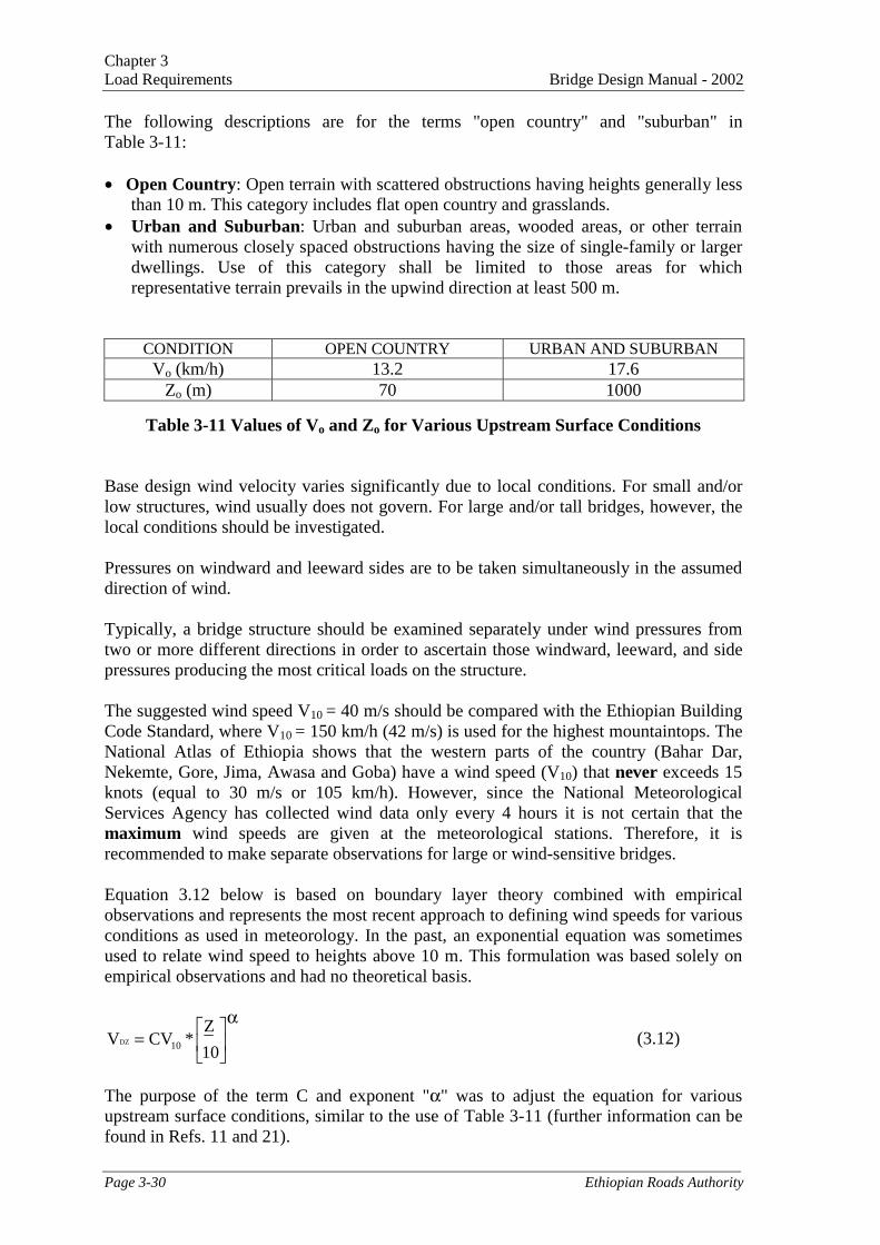
The following descriptions are for the terms "open country" and "suburban" inTable 3-11:
• Open Country: Open terrain with scattered obstructions having heights generally lessthan 10 m. This category includes flat open country and grasslands.
• Urban and Suburban: Urban and suburban areas, wooded areas, or other terrainwith numerous closely spaced obstructions having the size of single-family or largerdwellings. Use of this category shall be limited to those areas for whichrepresentative terrain prevails in the upwind direction at least 500 m.
CONDITION OPEN COUNTRY URBAN AND SUBURBANVo (km/h) 13.2 17.6
Zo (m) 70 1000
Table 3-11 Values of Vo and Zo for Various Upstream Surface Conditions
Base design wind velocity varies significantly due to local conditions. For small and/orlow structures, wind usually does not govern. For large and/or tall bridges, however, thelocal conditions should be investigated.
Pressures on windward and leeward sides are to be taken simultaneously in the assumeddirection of wind.
Typically, a bridge structure should be examined separately under wind pressures fromtwo or more different directions in order to ascertain those windward, leeward, and sidepressures producing the most critical loads on the structure.
The suggested wind speed V10 = 40 m/s should be compared with the Ethiopian BuildingCode Standard, where V10 = 150 km/h (42 m/s) is used for the highest mountaintops. TheNational Atlas of Ethiopia shows that the western parts of the country (Bahar Dar,Nekemte, Gore, Jima, Awasa and Goba) have a wind speed (V10) that never exceeds 15knots (equal to 30 m/s or 105 km/h). However, since the National MeteorologicalServices Agency has collected wind data only every 4 hours it is not certain that themaximum wind speeds are given at the meteorological stations. Therefore, it isrecommended to make separate observations for large or wind-sensitive bridges.
Equation 3.12 below is based on boundary layer theory combined with empiricalobservations and represents the most recent approach to defining wind speeds for variousconditions as used in meteorology. In the past, an exponential equation was sometimesused to relate wind speed to heights above 10 m. This formulation was based solely onempirical observations and had no theoretical basis.
�
���
�=
10
Z*CVV 10DZ (3.12)
The purpose of the term C and exponent "α" was to adjust the equation for variousupstream surface conditions, similar to the use of Table 3-11 (further information can befound in Refs. 11 and 21).

Chapter 3Bridge Design Manual - 2002 Load Requirements
Ethiopian Roads Authority Page 3-31
Wind Pressure on Structures: WS
For small and medium sized concrete bridges below 50m length the wind load onstructures shall be neglected.
For large and/or light bridges the following shall apply. If justified by local conditions, adifferent base design wind velocity shall be selected for load combinations not involvingwind on live load. The direction of the design wind shall be assumed horizontal, unlessotherwise specified in the following subchapter Aeroelastic Instability. In the absence ofmore precise data, design wind pressure, PD in kPa, shall be determined as:
25600VP
V
VPP DZ
2
B
2
B
DZBD =�
�
���
�= (3.13)
Where PB = base wind pressure specified in Table 3-12 (kPa):
STRUCTURAL COMPONENT WINDWARD LOAD, kPa LEEWARD LOAD, kPaTrusses, Columns, and Arches 2.4 1.2Beams 2.4 Not applicableLarge Flat Surfaces 1.9 Not applicable
Table 3-12 Base Pressures, PB Corresponding to VB = 160 km/h (45 m/s)
The wind loading shall not be taken less than 4.4 kN/m2 in the plane of a windward chordand 2.2 kN/m2 in the plane of a leeward chord on truss and arch components, and notless than 4.4 kN/m2 on beam or girder components.
Wind tunnel tests shall be used to provide more precise estimates of wind pressures. Suchtesting should be considered where wind is a major design load.
Where the wind is not taken as normal to the structure, the base wind pressures, PB, forvarious angles of wind direction shall be taken as specified in Table 3-13 and shall beapplied to a single place of exposed area. The skew angle shall be taken as measuredfrom a perpendicular to the longitudinal axis. The wind direction for design shall be thatwhich produces the extreme force effect on the component under investigation. Thetransverse and longitudinal pressures shall be applied simultaneously.
(kPa) Columns and Arches GirdersSkew Angle of Wind,
DegreesLateralLoad
LongitudinalLoad
Lateral Load LongitudinalLoad
0 3.6 0 2.4 015 3.4 0.6 2.1 0.330 3.1 1.3 2.0 0.645 2.3 2.0 1.6 0.860 1.1 2.4 0.8 0.9
Table 3-13 Base Wind Pressures, PB (kPa) for Various Angles of Attack VB=160km/h.

Chapter 3Load Requirements Bridge Design Manual - 2002
Page 3-32 Ethiopian Roads Authority
For trusses, columns, and arches, the base wind pressures specified in Table 3-13 are thesum of the pressures applied to both the windward and leeward areas.
The transverse and longitudinal forces to be applied directly to the substructure shall becalculated from an assumed base wind pressure of 1.9 kPa. For wind directions takenskewed to the substructure, this force shall be resolved into components perpendicular tothe end and front elevations of the substructure. The component perpendicular to the endelevation shall act on the exposed substructure area as seen in end elevation, and thecomponent perpendicular to the front elevation shall act on the exposed areas and shall beapplied simultaneously with the wind loads from the superstructure.
Wind Pressure on Vehicles: WL
When vehicles are present, the design wind pressure shall be applied to both structureand vehicles. Wind pressure on vehicles shall be represented by an interruptible, movingforce of 1.5 kN/m acting normal to, and 1.8 m above, the roadway and shall betransmitted to the structure.
When wind on vehicles is not taken as normal to the structure, the components of normaland parallel force applied to the live load shall be taken as specified in Table 3-14 withthe skew angle taken as referenced normal to the surface.
Skew Angle (Degrees) Normal Component (kN/m) Parallel Component (kN/m)0 1.46 015 1.28 0.1830 1.20 0.3545 0.96 0.4760 0.50 0.55
Table 3-14 Wind Components on Live Load
Based on practical experience, maximum live loads are not expected to be present on thebridge when the wind velocity exceeds 90 km/h. The load factor corresponding to thetreatment of wind on structure only in Load Combination Strength III would be(90/145)2*1.4 = 0.54, which has been rounded to 0.5 in the Strength IV LoadCombination. This load factor corresponds to 0.3 in Service 1.
The 1.5 kN/m wind load is based on a long row of randomly sequenced passenger cars,commercial vans, and trucks exposed to the 90-km/h design wind (25 m/s). Thishorizontal live load, similar to the design lane load, should be applied only to thetributary areas producing a force effect of the same kind.
3.18.2 VERTICAL WIND PRESSURE
Unless otherwise determined in following subchapter Aeroelastic Instability, a verticalupward wind force of 1.0 kPa (kN/m2) times the width of the deck, including parapetsand sidewalks, shall be considered a longitudinal line load. This force shall be appliedonly for large and/or other than concrete bridges. It shall be applied only for limit statesthat do not involve wind on live load, and only when the direction of wind is taken to beperpendicular to the longitudinal axis of the bridge. This lineal force shall be applied at

Chapter 3Bridge Design Manual - 2002 Load Requirements
Ethiopian Roads Authority Page 3-33
the windward quarter-point of the deck width in conjunction with the horizontal windloads specified in the previous subchapter Horizontal Wind Pressure.
The intent of this subchapter is to account for the effect resulting from interruption of thehorizontal flow of air by the superstructure. This load is to be applied even todiscontinuous bridge decks, such as grid decks. This load may govern whereoverturning of the bridge is investigated.
3.18.3 AEROELASTIC INSTABILITY
General
Aeroelastic force effects shall be taken into account in the design of bridges andstructural components that are wind-sensitive. For the purpose of this chapter, all bridges,and structural components thereof with a span length to width or depth ratio exceeding30.0 shall be deemed wind-sensitive.
The vibration of cables due to the interaction of wind and rain shall also be considered.
Because of the complexity of analyses often necessary for an in-depth evaluation ofstructural aeroelasticity, this subchapter is intentionally kept to a simple statement. Manybridges, decks, or individual structural components have been shown to be aeroelasticallyinsensitive if their length-to-width or length-to-depth ratios are under about 30.0, asomewhat arbitrary value helpful only in identifying likely wind-sensitive cases.
Aeroelastic Phenomena
The aeroelastic phenomena of vortex excitation, galloping, flutter, and divergence shallbe considered where applicable.
Control of Dynamic Responses
Bridges and structural components thereof, including cables, shall be designed to be freeof fatigue damage due to vortex-induced or galloping oscillations. Bridges shall bedesigned to be free of divergence and catastrophic flutter up to 1.2 times the design windvelocity applicable at bridge deck height. Slender structures and/or railway bridges shallbe checked for oscillations.
The self-frequency of any component or the whole bridge shall normally be less than 3.5Hz.Cables in stayed-girder bridges have been successfully stabilized against excessivedynamic responses by attaching automotive dampers to the bridge at deck level or bycross-tying multiple cable-stays.
Wind Tunnel Tests
Representative wind tunnel tests shall be used to satisfy the requirements of subchaptersAeroelastic Phenomena and Control of Dynamic Responses.

Chapter 3Load Requirements Bridge Design Manual - 2002
Page 3-34 Ethiopian Roads Authority
Wind tunnel testing of bridges and other civil engineering structures is a highlydeveloped technology, which shall be used to study the wind response characteristics of astructural model or to verify the results of analysis (Ref. 21).
3.19 EARTHQUAKE EFFECTS (EQ= EARTHQUAKE)
3.19.1 GENERAL
Earthquake loads shall be taken to be horizontal force effects determined on the basis ofthe elastic response coefficient, Csm, specified in the Elastic Seismic Response Coefficientsection of this subchapter, and the equivalent weight of the superstructure, adjusted bythe response modification factor, R, specified in the Response Modification Factorsection of this subchapter.
The provisions herein shall apply to bridges of conventional slab, beam girder, boxgirder, and truss superstructure construction with spans not exceeding 150 m. Theseprovisions need not be applied to completely buried structures.
Seismic effects for box culverts and buried structures need not be considered, exceptwhere they cross active faults.
The potential for soil liquefaction and slope movements shall be considered.
Earthquake loads are given by the product of the elastic seismic response coefficient Csm
and the equivalent weight of the superstructure. The equivalent weight is a function ofthe actual weight and bridge configuration and is automatically included in both thesingle-mode and multimode methods of analysis specified in subchapter Analysis forEarthquake Loads below.
These Specifications establish design and detailing provisions for bridges to minimizetheir susceptibility to damage from earthquakes. A flow chart summarizing theearthquake design provision is presented in Figure 3-8.
The design earthquake motions and forces specified herein are based on a low probabilityof their being exceeded during the normal life expectancy of a bridge. Bridges that aredesigned and detailed in accordance with the provisions of these Specifications maysuffer damage, but should have low probability of collapse due to seismically inducedground shaking.
The principles used for the development of these Specifications are:
• Small to moderate earthquakes should be resisted within the elastic range of thestructural components without significant damage.
• Realistic seismic ground motion intensities and forces should be used in the designprocedures.
• Exposure to shaking from large earthquakes should not cause collapse of all or part ofthe bridge. Where possible, damage that does occur should be readily detectable andaccessible for inspection and repair.

Chapter 3Bridge Design Manual - 2002 Load Requirements
Ethiopian Roads Authority Page 3-35
3.19.2 ACCELERATION COEFFICIENT
The coefficient, "A", to be used in the application of these provisions shall be determinedfrom the contour map of Ethiopia in Figure 3-9. Linear interpolation shall be used forsites located between contour lines or between a contour line and a local maximum orminimum.
Special studies to determine site- and structure-specific acceleration coefficients shall beperformed if any one of the following conditions exist:
• The site is located close to an active fault.
• Long-duration earthquakes are expected in the region.
• The importance of the bridge is such that a longer exposure period (and, therefore,return period) should be considered.
The effect of soil conditions at the site are considered in the following subchapter entitledSite Effects: Soil Profiles.
3.19.3 IMPORTANCE CATEGORIES
For the purpose of Section 3.10: Earthquake Effects, ERA or those having jurisdictionshall classify the bridges within Zone 4 (mainly Rift Valley) into one of three importancecategories as follows:
• Critical bridges,
• Essential bridges, or
• Other bridges.
The basis of classification shall include social/survival and security/defenserequirements. In classifying a bridge, consideration should be given to possible futurechanges in conditions and requirements.
Essential bridges are generally those that should, as a minimum, be open to emergencyvehicles and for security/defense purposes immediately after the design earthquake, i.e., a475-year return period event. However, some bridges must remain open to all traffic afterthe design earthquake and be usable by emergency vehicles and for security/defensepurposes immediately after a large earthquake, e.g., a 2500 year return period event.These bridges should be regarded as critical structures.
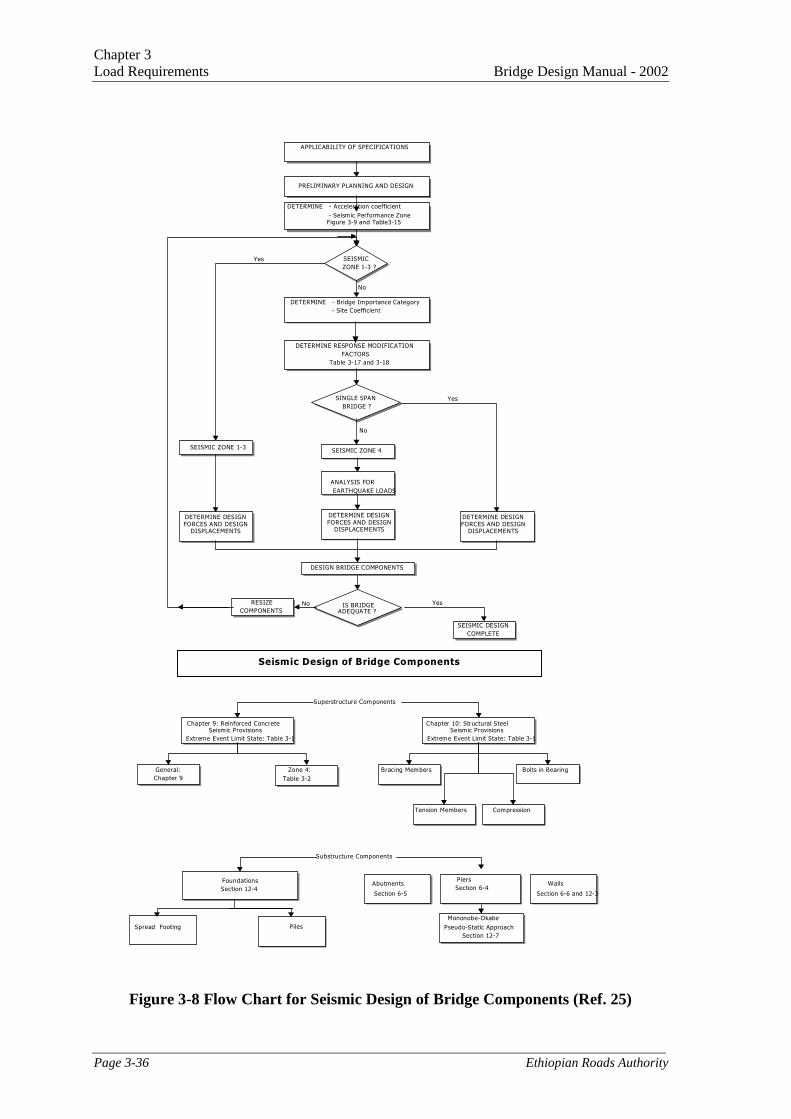
Chapter 3Load Requirements Bridge Design Manual - 2002
Page 3-36 Ethiopian Roads Authority
Figure 3-8 Flow Chart for Seismic Design of Bridge Components (Ref. 25)
APPLICABILITY OF SPECIFICATIONS
PRELIMINARY PLANNING AND DESIGN
DETERMINE - Acceleration coefficient - Seismic Performance Zone
Figure 3-9 and Table3-15
SEISMICZONE 1-3 ?
DETERMINE - Bridge Importance Category - Site Coefficient
DETERMINE RESPONSE MODIFICATIONFACTORS
Table 3-17 and 3-18
SINGLE SPANBRIDGE ?
SEISMIC ZONE 4
EARTHQUAKE LOADSANALYSIS FOR
FORCESArticle 3.10.9.3
SEISMIC ZONE 1-3
DESIGN BRIDGE COMPONENTS
IS BRIDGEADEQUATE ?
RESIZECOMPONENTS
DETERMINE DESIGNFORCES AND DESIGN
DISPLACEMENTS
Yes
No
No
Yes
SEISMIC DESIGNCOMPLETE
No Yes
Superstructure Components
Chapter 9: Reinforced ConcreteSeismic Provisions
Extreme Event Limit State: Table 3-1
General:Chapter 9
Zone 4:Table 3-2
Chapter 10: Structural SteelSeismic Provisions
Extreme Event Limit State: Table 3-1
Bracing Members Bolts in Bearing
Tension Members Compression
DETERMINE DESIGNFORCES AND DESIGN
DISPLACEMENTS
DETERMINE DESIGNFORCES AND DESIGN
DISPLACEMENTS
Seismic Design of Bridge Components
Substructure Components
FoundationsSection 12-4
Spread Footing Pseudo-Static ApproachSection 12-7
Abutments
Section 6-5
Piers Section 6-4
Walls
Section 6-6 and 12-3
Piles Mononobe-Okabe

Chapter 3Bridge Design Manual - 2002 Load Requirements
Ethiopian Roads Authority Page 3-37
(Ref. 23)
Figure 3-9 Earthquake Zones (Note: In zone 1-3 A≤0.07 and in zone 4 A≤0.10)
3.19.4 SEISMIC PERFORMANCE ZONES
Each bridge shall be assigned to one of the seismic zones in accordance with Table 3-15below:
EBCS zone from Figure 3-9 Acceleration Coefficient1 A ≤ 0.032 0.03 < A ≤ 0.053 0.05 < A ≤ 0.074 0.07 < A ≤ 0.10
Table 3-15 Seismic Zones

Chapter 3Load Requirements Bridge Design Manual - 2002
Page 3-38 Ethiopian Roads Authority
These seismic zones, from the Ethiopian Building Code Standards (Ref. 23) have areference return period of 100 years. They reflect the variation in seismic risk across thecountry and are used to permit different requirements for methods of analysis, minimumsupport lengths, column design details, foundation and abutment design procedures.
The zones 1-2 with a ground acceleration less than 0.05*g are considered as lowseismicity zones. In general, the ground acceleration tends to coincide with the actualpeak for moderate-to-high magnitude of medium-to-long distance events.
3.19.5 SITE EFFECTS: SOIL PROFILES
Site effects shall be included in the determination of seismic loads for bridges. Siteeffects on structural response are due to the soil conditions. Four soil profiles are used inthese Specifications to define a site coefficient used to modify the accelerationcoefficient.
The site coefficient, S, is used to include the effect of site conditions on the elasticseismic response coefficient as specified in the following subchapter.
The site coefficient, S, specified in Table 3-16 (below), shall be based upon soil profiletypes defined below.
Soil Profile TypeSiteCoefficient I II III IV
S 1.0 1.2 1.5 2.0
Table 3-16 Site Coefficients
In locations where the soil properties are not known in sufficient detail to determine thesoil profile type, or where the profile does not fit any of the four types, the site coefficientfor Soil Profile Type II shall be used.
A soil profile shall be taken as Type I if composed of rock of any description, eithershale-like or crystalline in nature, or stiff soils where the soil depth is less than 60 m, andthe soil types overlying the rock are stable deposits of sands, gravels, or stiff clays.These materials shall be characterized by a shear wave velocity greater than 765 m/s.
A profile with stiff cohesive or deep cohesionless soils where the soil depth exceeds 60 mand the soil types overlying the rock are stable deposits of sands, gravels, or stiff claysshall be taken as Type II.
A profile with soft to medium-stiff clays and sands, characterized by 9 m or more of softto medium-stiff clays with or without intervening layers of sand or other cohesionlesssoils shall be taken as Type III.
A profile with soft clays or silts greater than 12 m in depth shall be taken as Type IV.These materials shall be characterized by a shear wave velocity of less than 152 m/s andmight include loose natural deposits or manmade, nonengineered fill.

Chapter 3Bridge Design Manual - 2002 Load Requirements
Ethiopian Roads Authority Page 3-39
3.19.6 ELASTIC SEISMIC RESPONSE COEFFICIENT
Unless specified otherwise as exceptions in this subchapter, the elastic seismic responsecoefficient, Csm, for the mth mode of vibration shall be taken as:
A5.2T
AS2.1C
3/2m
sm ≤= (3.14)
where:Tm = period of vibration of the mth mode (s)A = acceleration coefficient specified in Table 3-15S = site coefficient specified in Table 3-16
The determination of the period of vibration, Tm, should be based on the nominal,unfactored mass of the component or structure.
The elastic seismic response coefficient shall be normalized using the input groundacceleration "A” and the result plotted against the period of vibration. Such a plot isgiven in Figure 3-10 for different soil profiles, based on 5 % damping.
An earthquake may excite several modes of vibration in a bridge and, therefore, theelastic response coefficient should be found for each relevant mode.
The structure is analyzed for these seismic forces in the single-mode method. In themultimode method, the structure is analyzed for several seismic forces, eachcorresponding to the period and mode shape of one of the fundamental modes ofvibration, and the results are combined using acceptable methods, such as the root-mean-square method.
Figure 3-10 Seismic Response Coefficients, Csm for Various Soil Profiles,Normalized with Respect to Acceleration Coefficient "A" (Csm on the leftaxis)

Chapter 3Load Requirements Bridge Design Manual - 2002
Page 3-40 Ethiopian Roads Authority
Exceptions to the application of Equation 3.14 are as follows:
• For bridges on soil profiles III or IV, Csm need not exceed 2.0*A.
• For soil profiles III and IV, and for modes other than the fundamental mode, thathave periods less than 0.3 s, Csm shall be taken as:
Csm = A (0.8 + 4.0*Tm) (3.15)
• If the period of vibration for any mode exceeds 4.0 s, the value of Csm for that modeshall be taken as:
Csm = 3AS (3.16)Tm
4/3
3.19.7 RESPONSE MODIFICATION FACTORS
To apply the response modification factors specified herein, the structural details shallsatisfy the provisions of seismic hooks, shall have a minimum reinforcement of at least0.25 % in both directions for Zone 4, and shall have additional pile reinforcementaccording to Section 6.3: Footings on Piles.
Except as noted herein, seismic design force effects for substructures and the connectionsbetween parts of structures shall be determined by dividing the force effects resultingfrom elastic analysis by the appropriate response modification factor, R, as specified inTables 3-17 and 3-18, respectively.
As an alternative to the use of the R-factors, specified in Table 3-18 for connections,monolithic joints between structural members and/or structures, such as a column-to-footing connection, shall be designed to transmit the maximum force effects that can bedeveloped by the inelastic hinging of the column or multicolumn bent they connect asspecified hereinafter in section on Longitudinal Restrainers.
If an inelastic time history method of analysis is used, the response modification factor,R, shall be taken as 1.0 for all substructure and connections.
Importance CategorySubstructureCritical Essential Other
Wall-type piers – larger dimension 1.5 1.5 2.0Reinforced concrete pile bents• Vertical piles only• With battered piles
1.51.5
2.01.5
3.02.0
Single columns 1.5 2.0 3.0Steel or composite steel and concrete pile bents• Vertical pile only• With battered piles 1.5
1.53.52.0
5.03.0
Multiple column bents 1.5 3.5 5.0
Table 3-17 Response Modification R-Factors for Substructures

Chapter 3Bridge Design Manual - 2002 Load Requirements
Ethiopian Roads Authority Page 3-41
Connection All Importance Categories
Superstructure to abutment 0.8
Expansion joints within a span of the superstructure 0.8
Columns, piers, or pile bents to cap beam or superstructure 1.0
Columns or piers to foundations 1.0
Table 3-18 Response Modification R-Factors for Connections
These Specifications recognize that it is uneconomical to design a bridge to resist largeearthquakes elastically. Columns are assumed to deform inelastically where seismicforces exceed their design level, which is established by dividing the elasticallycomputed force effects by the appropriate R-factor.
R-factors for connections are smaller than those for substructure members in order topreserve the integrity of the bridge under these extreme loads. For expansion jointswithin the superstructure and connections between the superstructure and abutment, theapplication of the "R" factor results in force effect magnification. Connections thattransfer forces from one part of a structure to another include, but are not limited to, fixedbearings and shear keys. For one-directional bearings, these R-factors are used in therestrained direction only. In general, forces determined based on plastic hinging will beless than those given by using Table 3-18, resulting in a more economical design.
Seismic loads shall be assumed to act in any lateral direction. The appropriate R-factorshall be used for both orthogonal axes of the substructure.
A wall-type concrete pier shall be analyzed as a single column in the weak direction if allthe provisions for columns are satisfied.
Usually the orthogonal axes will be the longitudinal and transverse axes of the bridge. Inthe case of a curved bridge, the longitudinal axis shall be the chord joining the twoabutments. Wall-type piers shall be treated as wide columns in the strong direction,provided the appropriate R-factor in this direction is used.
3.19.8 COMBINATION OF SEISMIC FORCE EFFECTS
The elastic seismic force effects on each of the principal axes of a component resultingfrom analyses in the two perpendicular directions shall be combined to form two loadcases as follows:
• 100 % of the absolute value of the force effects in one of the perpendicular directionscombined with 30 % of the absolute value of the force effects in the secondperpendicular direction, and
• 100 % of the absolute value of the force-effects in the second perpendicular directioncombined with 30 % of the absolute value of the force effects in the firstperpendicular direction.

Chapter 3Load Requirements Bridge Design Manual - 2002
Page 3-42 Ethiopian Roads Authority
3.19.9 CALCULATION OF DESIGN FORCES
General
For single-span bridges, regardless of seismic zone, the minimum design connectionforce effect in the restrained direction between the superstructure and the substructureshall not be less than the product of the site coefficient, the acceleration coefficient, andthe tributary permanent load.
Seat widths at expansion bearings of multispan bridges shall either comply with theminimum displacement requirements in the following subchapter entitled Analysis forEarthquake Loads, or longitudinal restrainers complying with subchapter entitled Hold-Down Devices shall be provided.
Special attention should be paid to certain substructures such as piers.
This subchapter refers to superstructure effects carried into substructure. Abutments onmultispan bridges, but not single-span bridges, and retaining walls are subject toacceleration-augmented soil pressures as specified in the subchapter entitled Effect ofEarthquake, below. Wingwalls on single-span structures are not fully covered at thistime, and the Designer should use judgment in this area.
Seismic Zone 1-3 in Figure 3-9
For bridges on sites in Zones 1-3 where the acceleration coefficient is less than 0.025 andthe soil profile is either Type I or II, the horizontal design connection force in therestrained directions shall not be taken to be less than 0.1 times the vertical reaction dueto the tributary permanent load and the tributary live loads assumed to exist during anearthquake.
For all other sites in Zones 1-3, the horizontal design connection force in the restraineddirections shall not be taken to be less than 0.2 times the vertical reaction due to thetributary permanent load and the tributary live loads assumed to exist during anearthquake.
For each uninterrupted segment of a superstructure, the tributary permanent load at theline of fixed bearings, used to determine the longitudinal connection design force, shallbe the total permanent load of the segment.
If each bearing supporting an uninterrupted segment or simply-supported span isrestrained in the transverse direction, the tributary permanent load used to determine theconnection design force shall be the permanent load reaction at that bearing.
Each elastomeric bearing and its connection to the masonry and sole plates shall bedesigned to resist the horizontal seismic design forces transmitted through the bearing.For all bridges in Seismic Zones 1-3 and all single span bridges, these seismic shearforces shall not be less than the connection force specified herein.
These provisions arise because seismic analysis for bridges in Zone 1-3 is generally notrequired. These default values are used as minimum design forces in lieu of rigorous

Chapter 3Bridge Design Manual - 2002 Load Requirements
Ethiopian Roads Authority Page 3-43
analysis. The division of Zone 1-3 at an acceleration coefficient 0.025 for sites withfavorable soil condition is an arbitrary expedience intended to provide some relief toparts of the country with very low seismicity.
If each bearing supporting a continuous segment or simply supported span is anelastomeric bearing, there are no restrained directions due to the flexibility of thebearings.
The magnitude of live load assumed to exist at the time of the earthquake should beconsistent with the value of γeq used in conjunction with Table 3-2.
Seismic Zone 4
Single span structures need not to be designed according to seismic analysis.Multispan structures in Seismic Zone 4 (in Figure 3-9 above) shall be analyzedaccording to single mode analysis or uniform load elastic method, or for irregularessential and all critical bridges according to multimode elastic method.
Except for foundations, seismic design forces for all components, including pile bentsand retaining walls, shall be determined by dividing the elastic seismic forces, obtainedfrom previous subchapter Combination of Seismic Forces Effects, by the appropriateresponse modification factor, R, specified in Table 3-16.
Seismic design forces for foundations, other than pile bents and retaining walls, shall bedetermined by dividing elastic seismic forces, obtained from previous subchapterCombination of Seismic Forces Effects, by half of the response modification factor, R,from Table 3-16, for the substructure component to which it is attached. The value ofR/2 shall not be taken as less than 1.0.
Where a group load other than EXTREME EVENT 1, specified in Table 3-1, governs thedesign of columns, the possibility that seismic forces transferred to the foundations shallbe larger than those calculated using the procedure specified above, due to possibleoverstrength of the columns, shall be considered.
Longitudinal Restrainers
Friction shall not be considered an effective restrainer. Restrainers shall be designed for aforce calculated as the acceleration coefficient times the permanent load of the lighter ofthe two adjoining spans or parts of the structure.
If the restrainer is at a point where relative displacement of the sections of superstructureis designed to occur during seismic motions, sufficient slack shall be allowed in therestrainer so that the restrainer does not start to act until the design displacement isexceeded.
Where a restrainer is to be provided at columns or piers, the restrainer of each span shallbe attached to the column or pier rather than to interconnecting adjacent spans.

Chapter 3Load Requirements Bridge Design Manual - 2002
Page 3-44 Ethiopian Roads Authority
Hold-Down Devices
For Seismic Zone 4, hold-down devices shall be provided at supports and at hinges incontinuous structures where the vertical seismic force due to the longitudinal seismicload opposes and exceeds 50 %, but is less than 100 %, of the reaction due to permanentloads. In this case, the net uplift force for the design of the hold-down device shall betaken as 10 % of the reaction due to permanent loads that would be exerted if the spanwere simply supported.
If the vertical seismic forces result in net uplift, the hold-down device shall be designedto resist the larger of either:
• 120 % of the difference between the vertical seismic force and the reaction due topermanent loads, or
• 10 % of the reaction due to permanent loads.
Figure 3-11 Example of hold-down device for expansion bearing:Principle and Picture
3.19.10 ANALYSIS FOR EARTHQUAKE LOADS
General
Minimum analysis requirements for seismic effects shall be as specified in Table 3-19.
For the modal methods of analysis specified in this subchapter, the elastic designspectrum shall be that given by Equation 3.14.
Bridges in Seismic Zone 1-3 need not be analyzed for seismic loads, regardless of theirimportance and geometry. However, the minimum requirements, as specified herein andin previous subchapter Calculation of Design Forces shall apply.
Single-Span Bridges
Seismic analysis is not required for single-span bridges, regardless of seismic zone.
Clearance
Slidingplates
Anchorage Bolts

Chapter 3Bridge Design Manual - 2002 Load Requirements
Ethiopian Roads Authority Page 3-45
Connections between the bridge superstructure and the abutments shall be designed forthe minimum force requirements as specified in previous subchapter Calculation ofDesign Forces.
Minimum seat width requirements shall be at least 500 mm at each abutment.
Multispan Bridges
For multispan structures, the minimum analysis requirements shall be as specified below:
Multispan BridgesOther Bridges Essential Bridges Critical Bridges
SeismicZone
Single-SpanBridges
Regular Irregular Regular Irregular Regular Irregular1-34
No Seismic AnalysisSeismic Analysis
*SM/UL
*SM
*SM/UL
*MM
*MM
*MM
Ref. 23Table 3-19 Minimum Analysis Requirements for Seismic Effects
in which:* = no seismic analysis required (Zone 1-3)UL = uniform load elastic methodSM = single-mode elastic methodMM = multimode elastic method
The selection of the method of analysis depends on seismic zone, regularity, andimportance of the bridge.
Regularity is a function of the number of spans and the distribution of weight andstiffness. Regular bridges have less than seven spans, no abrupt or unusual changes inweight, stiffness, or geometry; and no large changes in these parameters from span tospan or support-to-support, abutments excluded. They are defined in Table 3-20.
Any bridge not satisfying the requirements of Table 3-20 is considered to be "irregular".A more rigorous analysis procedure shall be used in lieu of the recommended minimum.
Sometimes special types of substructures (high masonry piers) need to be designed forseismic load.
A curved bridge shall be analyzed as if it were straight, provided all of the followingrequirements are satisfied:
• The bridge is regular as defined in Table 3-20, except that for a two-span bridge themaximum span length ratio from span to span must not exceed 2;
• The subtended angle in plan is not greater than 90°, andThe span lengths of the equivalent straight bridge are equal to the arc lengths of the
curved bridge.
If these requirements are not satisfied, then curved bridges must be analyzed using theactual curved geometry.

Chapter 3Load Requirements Bridge Design Manual - 2002
Page 3-46 Ethiopian Roads Authority
Parameter ValueNumber of Spans 2 3 4 5 6
Maximum subtended angle for a curved bridge 90o 90o 90o 90o 90o
Maximum span length ratio from span to span 3 2 2 1.5 1.5Maximum bent/pier stiffness ratio from span tospan, excluding abutments
-- 4 4 3 2
Table 3-20 Regular Bridge Requirements
Single-Mode Methods of Analysis (SM)
Either of the two single-mode methods of analysis specified herein (Single-Mode Methodof Spectral Analysis and Uniform Load Method) shall be used where appropriate.
The Single-Mode Method of Spectral Analysis (SM) shall be based on the fundamentalmode of vibration in either the longitudinal or transverse direction. This mode shape shallbe found by applying a uniform horizontal load to the structure and calculating thecorresponding deformed shape. The natural period shall be calculated by equating themaximum potential and kinetic energies associated with the fundamental mode shape.
The amplitude of the displaced shape shall be found from the elastic seismic responsecoefficient, Csm, specified in previous subchapter Elastic Seismic Response Coefficient,and the corresponding spectral displacement. This amplitude shall be used to determineforce effects.The steps described below shall be followed:
Step 1
Calculate the static displacements Vs(X) due to an assumed uniform loading Po as shownin figure 3-12.
Figure 3-12

Chapter 3Bridge Design Manual - 2002 Load Requirements
Ethiopian Roads Authority Page 3-47
Step 2
Calculate factors α, β and γ as:
α = �Vs(x)dx
β = � Vs(x)dxW(x)
γ = � Vs²(x)dxW(x)
where:
Po = a uniform load arbitrarily set equal to 1.0 (N/m)Vs(x) = deformation corresponding to Po (m)W(x) = nominal, unfactored dead load of the bridge superstructure and tributary
substructure (N/m)
The computed factors α, β and γ have units of (m²), (N.m) and (N.m²) respectively.
Step 3
Calculate the period of the bridge as:
Tm =623.31
2πα
γgPo
Where:
g = acceleration of gravity (N/S²)
Step 4
Using Tm and Equation 3.14, calculate Csm
Step 5
Calculate the equivalent static earthquake loading pe(x) as:
pe(x) = γβ smC
W(x) Vs(x)
where:
Csm = the dimensionless elastic seismic response coefficient given by Equation 3.14
pe(x) = the intensity of the equivalent static seismic loading applied to represent theprimary mode of vibration (N/m)

Chapter 3Load Requirements Bridge Design Manual - 2002
Page 3-48 Ethiopian Roads Authority
Step 6
Apply loading pe(x) to the structure, and determine the resulting member force effects.
Uniform Load Method (UL)
The Uniform Load Method (UL) shall be used on the fundamental mode of vibration ineither the longitudinal or transverse direction. The period of this mode of vibration shallbe taken as that of an equivalent single mass-spring oscillator. The stiffness of thisequivalent spring shall be calculated using the maximum displacement that occurs whenan arbitrary uniform lateral load is applied to the bridge. The elastic seismic responsecoefficient Csm, specified in previous subchapter Elastic Seismic Response Coefficient,shall be used to calculate the equivalent uniform seismic load from which seismic forceeffects are found.
It is essentially an equivalent static method of analysis that uses a uniform lateral load toapproximate the effect of seismic loads. The method is suitable for regular bridges thatrespond principally in their fundamental mode of vibration. Whereas all displacementsand most member forces are calculated with good accuracy, the method is known tooverestimate the transverse shears at the abutments by up to 100 percent. If suchconservatism is undesirable, then the single-mode spectral analysis method specifiedabove is recommended.
The steps described below shall be followed:
Step 1
Calculate the static displacements vs(x) due to an assumed uniform load po, as known inFigure 3.12. The uniform loading po is applied over the length of the bridge; it has unitsof force/unit length and may be arbitrarily set equal to 1.0. The static displacement vs(x)has units of length.
Step 2
Calculate the bridge lateral stiffness, K, and total weight, W, from the followingexpressions:
K =MAXs
o
VLp
,
W = � dxxw )(
where:
L = total length of the bridge (m)Vs, MAX = maximum value of vs(x) (m)W(x) = nominal, unfactored dead load of the bridge superstructure and tributary
substructure (N/m)
The weight should take into account structural elements and other relevant loadsincluding, but not limited to, pier caps, abutments, columns, and footings. Other loads,such as live loads, may be included. Generally, the inertia effects of live loads are notincluded in this analysis; however, the probability of a large live load being on the bridge
Chapter 3Bridge Design Manual - 2002 Load Requirements
Ethiopian Roads Authority Page 3-49
during an earthquake should be considered when designing bridges with high live-to-dead load ratios that are located in metropolitan areas where traffic congestion is likely tooccur.
Step 3
Calculate the period of the bridge, Tm, using the expression:
gKWTm π2=
where:
g = acceleration of gravity (m/s²)
Step 4
Calculate the equivalent static earthquake loading pe from the expression:
gKWCp sm
e =
where:
Csm = the dimensionless elastic seismic response coefficient given by Equation 3.14Pe = equivalent uniform static seismic loading per unit length of bridge applied to
represent the primary mode of vibration (N/m)
Step 5
Calculate the displacements and member forces for use in design either by applying pe tothe structure and performing a second static analysis or by scaling the results of the firststep above by the ration pe/po.
Multimode Spectral Method
The Multimode Spectral Analysis Method (MM) shall be used for bridges in whichcoupling occurs in more than one of the three coordinate directions within each mode ofvibration. As a minimum, linear dynamic analysis using a three-dimensional model shallbe used to represent the structure.The number of modes included in the analysis should be at least three times the numberof spans in the model.The elastic response spectrum as specified in previous subchapter Elastic SeismicResponse Coefficient shall be used for each mode.
The member forces and displacements may be estimated by combining the respectiveresponse quantities (moment, force, displacement, or relative displacement) from theindividual modes by the Complete Quadratic Combination (CQC) method.
Member forces and displacements obtained using the CQC combination method aregenerally adequate for most bridge systems (Wilson et al. 1981).
3.19.11 REQUIREMENTS FOR TEMPORARY BRIDGES AND STAGE CONSTRUCTION
Any bridge or partially constructed bridge that is expected to be temporary for more thanfive years shall be designed using the requirements for permanent structures and shall not

Chapter 3Load Requirements Bridge Design Manual - 2002
Page 3-50 Ethiopian Roads Authority
use the provisions of this Chapter. The option to use a reduced acceleration coefficient isprovided to reflect the limited exposure period.
The requirement that an earthquake shall not cause collapse of all or part of a bridge, asstated in the beginning of this Section 3.19: Earthquake Effects, shall apply to temporarybridges expected to carry traffic. It shall also apply to those bridges that are constructedin stages and expected to carry traffic and/or pass over routes that carry traffic. Theacceleration coefficient given in previous subchapter Acceleration Coefficient shall bereduced by a factor of not more than 2 in order to calculate the component elastic forcesand displacements. Acceleration coefficients for construction sites that are close toactive faults shall be the subject of special study. The response modification factors givenin previous subchapter Response Modification Factors shall be increased by a factor ofnot more than 1.5 in order to calculate the design forces. This factor shall not be appliedto connections as defined in Table 3-18.
The minimum seat width in zone 4 shall be at least 0.6 m for all temporary bridges andstaged construction.
3.20 EARTH PRESSURE (EH = HORIZONTAL EARTH PRESSURE; ES = EARTH SURCHARGE;LS = LIVE LOAD SURCHARGE; DD = DOWNDRAG)
3.20.1 GENERAL
Earth pressure shall be considered as a function of the:
• Type and density of earth,• Water content,• Soil creep characteristics,• Degree of compaction
• Location of groundwater table,• Earth-structure interaction,• Amount of surcharge, and• Earthquake effects.
Walls that can tolerate little or no movement should be designed for at-rest earthpressure. Walls that can move away from the soil mass should be designed for pressuresbetween active and at-rest conditions, depending on the magnitude of the tolerablemovements. Movement required to reach the minimum active pressure or the maximumpassive pressure is a function of the wall height and the soil type. Some typical values ofthese mobilizing movements, relative to wall height, are given in Table 3-21:
Values of ∆/HType of Backfill Active Passive
Dense sand 0.001 0.01Medium-dense sand 0.002 0.02Loose sand 0.004 0.04Compacted silt 0.002 0.02Compacted lean clay 0.010 0.05Compacted fat clay 0.010 0.05
Table 3-21 Approximate Values of Relative Movements Required to ReachMinimum Active or Maximum Passive Earth Pressure Conditions (Ref 5)

Chapter 3Bridge Design Manual - 2002 Load Requirements
Ethiopian Roads Authority Page 3-51
Where:
∆ = movement of top of wall required to reach minimum active or maximum passivepressure by tilting or lateral translation (mm)H = height of wall (mm)
For walls that are backfilled with cohesive materials, the effects of soil creep should betaken into consideration in estimating the design earth pressures.
Under stress conditions close to the minimum active or maximum passive earthpressures, the cohesive soils indicated in Table 3-21 creep continually, and themovements shown produce active or passive pressures only temporarily. If there is nofurther movement, active pressures will increase with time, approaching the at-restpressure, and passive pressures will decrease with time, approaching values on the orderof 40 % of the maximum short-term value.
3.20.2 COMPACTION
Where activity by mechanical compaction equipment is anticipated within a distance ofone-half the height of the wall, taken as the difference in elevation between the pointwhere finished grade intersects the back of the wall and the base of the wall, the effect ofadditional earth pressure that shall be induced by compaction shall be taken into account.
The heavier the equipment used to compact the backfill, and the closer it operates to thewall, the larger are the compaction-induced pressures. The magnitude of the earthpressures exerted on a wall by compacted backfill can be minimized by using only smallrollers or hand compactors within a distance of one-half wall height from the back of thewall.
3.20.3 PRESENCE OF WATER
Wherever possible, the development of hydrostatic water pressure on walls should beeliminated through use of free-draining (rapid-draining) backfill material and/or the useof weep holes and crushed rock, pipe drains, gravel drains, perforated drains, or geofabricdrains that provide drainage.
If the retained earth is not dewatered, the effect of hydrostatic water pressure shall beadded to that of earth pressure as indicated in Figure 3-13. In cases where water isexpected to pond behind a wall, the wall shall be designed to withstand the hydrostaticwater pressure plus the earth pressure. Submerged densities of the soil shall be used todetermine the lateral earth pressure below the groundwater table.
If the groundwater levels differ on opposite sides of the wall, the effects of seepage onwall stability and the potential for piping shall be considered. Pore pressures behind thewall shall be approximated by flow net procedures or various analytical methods andshall be added to the effective horizontal stresses in determining total lateral earthpressures on the wall.

Chapter 3Load Requirements Bridge Design Manual - 2002
Page 3-52 Ethiopian Roads Authority
Figure 3-13 Effect of Groundwater Table
3.20.4 EFFECT OF EARTHQUAKE
The effects of probable amplification of active earth pressure and/or mobilization ofpassive earth masses by earthquake shall be considered.
The Mononobe-Okabe method for determining equivalent static fluid pressures forseismic loads on gravity and semigravity retaining walls is presented under Section 12.5:Substructures for RC Bridges. The Mononobe-Okabe analysis is based, in part, on theassumption that the backfill soils are not susceptible to liquefaction.
Where soils are subject to both saturation and seismic or other cyclic/instantaneous loads,special consideration should be given to addressing the possibility of soil liquefaction.
3.20.5 EARTH PRESSURE: EH
Basic Earth Pressure
Basic earth pressure (p, in MPa) shall be assumed to be linearly proportional to the depthof earth and taken as:
p = kh*γs*g*z *10-9 (3.17)
where: kh = coefficient of lateral earth pressure taken as ko, specified in Table 3-22, forwalls that do not deflect or move, or ka, specified in Equations 3.20 and 3.26,and ka, specified in Equation 3.28, for walls that deflect or move sufficiently toreach minimum active conditions.
γs = density of soil (kg/m3)z = depth below the surface of earth (mm)g = Gravitational acceleration (m/s2)
Unless otherwise specified, the resultant lateral earth load due to the weight of thebackfill shall be assumed to act at a height of 0.4*H above the base of the wall, where His the total wall height measured from the surface of the ground to the bottom of thefooting.

Chapter 3Bridge Design Manual - 2002 Load Requirements
Ethiopian Roads Authority Page 3-53
The triangular distribution of lateral earth pressure is a simplification of the actualnonlinear distribution depicted in Figure 3-14. Two factors contribute to the nonlinearbehavior: (1) arching due to shear stresses in the soil at the foundation level and on theplane above the wall heel, and (2) compaction-induced lateral earth pressure in thebackfill. When the backfill moves laterally with the wall, it does not move freely on africtionless horizontal plane at the foundation level.
Shear stresses exist in the soil at this level. Shear stress can also exist on the verticalplane above the wall heel. Together, these shear stresses tend to reduce the lateral earthpressure at the bottom of the wall. This phenomenon is sometimes referred to as soilarching. Compaction-induced lateral earth pressures are most significant near the top ofthe wall. The combination of these two effects is shown by the nonlinear curve in Figure3-14. The resultant of the lateral earth force Ph can be obtained from the simplifiedtriangular distribution. However, to be equivalent to the actual nonlinear distribution inmoment calculations, the location of the resultant must be raised from 0.33*H to 0.4*H(Refs. 20 and 22).
Figure 3-14 Location of Resultant for Horizontal Earth Pressure
At-Rest Pressure Coefficient, k0.
For normally consolidated soils, the coefficient of lateral at-rest earth pressure shall betaken as:
ko = 1-sinϕf (3.18)
where: ϕf = friction angle of drained soilko = coefficient of earth pressure at rest for overconsolidated soils
For overconsolidated soils, the coefficient of lateral at-rest earth pressure shall beassumed to vary as a function of the overconsolidation ratio (OCR) or stress history, andshall be taken as:
ko = (1 - sinϕf) (OCR)sinϕf (3.19)
where: OCR = overconsolidation ratio
Values of ko for various overconsolidation ratios, OCR, shall be taken from Table 3-22.
Silt, lean clay, and highly plastic clay should not be used for backfill where free-draininggranular materials are available.

Chapter 3Load Requirements Bridge Design Manual - 2002
Page 3-54 Ethiopian Roads Authority
Coefficient of Lateral Earth Pressure, koSoil typeOCR = 1 OCR = 2 OCR = 5 OCR = 10
Loose sand 0.45 0.65 1.10 1.60Medium Sand 0.40 0.60 1.05 1.55Dense Sand 0.35 0.55 1.00 1.50Silt (ML) 0.50 0.70 1.10 1.60Lean Clay (CL) 0.60 0.80 1.20 1.65Highly Plastic Clay (CH) 0.65 0.80 1.10 1.40
(Ref 5)
Table 3-22 Typical Coefficients of Lateral Earth Pressure At-Rest (ko)
For typical cantilevered walls over 1.5 m high with structural-grade backfill, calculationsindicate that the horizontal movement of the top of the wall due to a combination ofstructural deformation of the stem and rotation of the foundation is sufficient to developactive conditions.
Active Pressure Coefficient, ka
Values for the coefficient of active pressure shall be taken as:
ka = sin2 (θ + ϕ/) (3.20)Γ* sin2θ sin (θ - δ)
in which:2
Γ = 1 + sin (ϕ/ + δ) sin (ϕ/ - β) (3.21)sin (θ - δ) sin (θ + β)
where: δ = friction angle between fill and wall taken as specified in Table 3-23 (°)β = angle of fill to the horizontal as shown in Figure 3-15 (°)θ = angle of backfill of wall to the vertical as shown in Figure 3-15 (°)ϕ/ = effective angle of internal friction (°)
Interface Materials FrictionAngle, δ
Mass concrete on the following foundation materials:• Clean sound rock• Clean gravel, gravel-sand mixtures, coarse sand• Clean fine to medium sand, silty medium to coarse sand, silty or clayey
gravel• Clean fine sand, silty or clayey fine to medium sand• Fine sandy silt, nonplastic silt• Very stiff and hard residual or preconsolidated clay• Medium stiff and stiff clay and silty clayMasonry on foundation materials has same friction factors
35°29 to 31°24 to 29°
19 to 24°17 to 19°22 to 26°17 ton 19°

Chapter 3Bridge Design Manual - 2002 Load Requirements
Ethiopian Roads Authority Page 3-55
Steel sheet piles against the following soils:• Clean gravel, gravel-sand mixtures, well-graded rock fill with spalls• Clean sand, silty sand-gravel mixture, single-size hard rock fill• Silty sand, gravel, or sand mixed with silt or clay• Fine sandy silt, nonplastic silt
22°17°14°11°
Formed or precast concrete(concrete sheet piling) against following soils:• Clean gravel, gravel-sand mixtures, well-graded rock fill with spalls• Clean sand, silty sand-gravel mixture, single-size hard rock fill• Silty sand, gravel, or sand mixed with silt or clay• Fine sandy silt, nonplastic silt
22 to 26°17 to 22°
17°14°
Various structural materials:• Masonry on masonry, igneous, and metamorphic rocks:
• Dressed soft rock on dressed soft rock• Dressed hard rock on dressed soft rock• Dressed hard rock on dressed hard rock
• Masonry on wood in direction of cross grain• Steel on steel at sheet pile interlocks
35°33°29°26°17°
Table 3-23 Friction Angle for Dissimilar Materials
For conditions that deviate from those described in Figure 3-15, the active pressure shallbe calculated by using a trial procedure based on wedge theory.
Figure 3-15 Notation for Coulomb at Earth Pressure
The values of ka determined from Equation 3.20 are based on the Coulomb earth pressuretheories. The theories are applicable for design of retaining walls. In general, Coulombwedge theory applies to gravity, semigravity, and prefabricated modular walls withrelatively steep back faces and to concrete cantilever walls with short heels.
For the cantilever wall in Figure 3-16, the earth pressure is applied to a plane extendingvertically from the heel of the wall base, and the weight of soil to the left of the verticalplane is considered as part of the wall weight.

Chapter 3Load Requirements Bridge Design Manual - 2002
Page 3-56 Ethiopian Roads Authority
Figure 3-16 Application of Coulomb Earth Pressure Theories in RetainingWall Design (Ref. 3)
Passive Pressure Coefficient, kp
For noncohesive soils, values of the coefficient of passive pressure shall be taken fromFigure 3-15 for the case of a sloping or vertical wall with a horizontal backfill or fromFigure 3-16 for the case of a vertical wall and sloping backfill. For conditions thatdeviate from those described in Figures 3-17 and 3-18, the passive pressure shall becalculated by using a trial procedure based on wedge theory. When wedge theory isused, the limiting value of the wall friction angle should not be taken larger than one-halfthe angle of internal friction, ϕ.
For cohesive soils, passive earth pressures, Pp (MPa) shall be estimated by:
_ (3.22)
where: γs = density of soil (kg/m3)Z = depth below surface of soil (mm)c = unit cohesion (MPa)kp = coefficient of passive pressure specified in Figures 3-17 and 3-18, as
appropriate
The movement required to mobilize passive pressure is approximately 10 times as largeas the movement needed to reduce earth pressure to the active values. The movementrequired to mobilize full passive pressure in loose sand is approximately 5 % of theheight of the face on which the passive pressure acts. For dense sand, the movementrequired to mobilize full passive pressure is smaller than 5 % of the height of the face onwhich the passive pressure acts. For poorly compacted cohesive soils, the movementrequired to mobilize full passive pressure is larger than 5 % of the height of the face onwhich the pressure acts. Wedge solutions are inaccurate and unconservative for largervalues of wall friction angle.
p9
spp k*c*210*Z*g**kP +γ= −

Chapter 3Bridge Design Manual - 2002 Load Requirements
Ethiopian Roads Authority Page 3-57
Figure 3-17 Computational Procedures for Passive Earth Pressures for SlopingWall with Horizontal Backfill
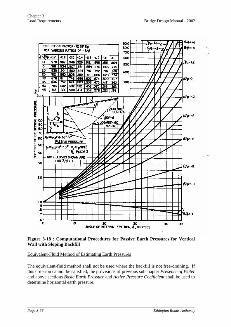
Chapter 3Load Requirements Bridge Design Manual - 2002
Page 3-58 Ethiopian Roads Authority
Figure 3-18 : Computational Procedures for Passive Earth Pressures for VerticalWall with Sloping Backfill
Equivalent-Fluid Method of Estimating Earth Pressures
The equivalent-fluid method shall not be used where the backfill is not free-draining. Ifthis criterion cannot be satisfied, the provisions of previous subchapter Presence of Waterand above sections Basic Earth Pressure and Active Pressure Coefficient shall be used todetermine horizontal earth pressure.

Chapter 3Bridge Design Manual - 2002 Load Requirements
Ethiopian Roads Authority Page 3-59
Where the equivalent-fluid method is used, the basic earth pressure, p (MPa), shall betaken as:
p = γeq *g *Z *10-9 (3.23)
where: γeq = equivalent-fluid density of soil, not less than 480 (kg/m3)
The resultant lateral earth load due to the weight of the backfill shall be assumed to act ata height of 0.4H above the base of the wall, where H is the total wall height measuredfrom the surface of the ground to the bottom of the footing. In the analysis of undrainedcohesive backfills, the earth pressure shall be calculated using equivalent-fluid pressure.
Typical values for equivalent-fluid densities for design of a wall of height not exceeding6.0 m shall be taken from Table 3-24 below, where:
∆ = movement of top of wall required to reach minimum active or maximumpassive pressure by tilting or lateral translation (mm)
H = height of wall (mm)i = angle of fill to the horizontal (°)
Level Backfill Backfill with i = 25o (≈1:2)Type of SoilAt-Rest
γeq(kg/m3)∆/H = 1/240γeq(kg/m3)
At-Restγeq(kg/m3)
∆/H = 1/240γeq(kg/m3)
Loose sand or gravel 880 640 1040 800
Medium dense sand or gravel 800 560 960 720
Dense sand or gravel 720 480 880 640
Compacted silt (ML) 960 640 1120 800
Compacted lean clay (CL) 1120 720 1280 880
Compacted fat clay (CH) 1280 880 1440 1040
Table 3-24 Typical Values for Equivalent-Fluid Densities of Soils
The magnitude of the vertical component of the earth pressure resultant for the case ofsloping backfill surface shall be determined as:
Pv = Ph tan i (3.24)
where: Ph = 0.5 γeq * g* H2* 10-9 (3.25)
Values of the density of equivalent fluids are given for walls that can tolerate very littleor no movement as well as for walls that can move as much as 25 mm in 6m. Theconcepts of equivalent-fluid densities have taken into account the effect of soil creep onwalls.

Chapter 3Load Requirements Bridge Design Manual - 2002
Page 3-60 Ethiopian Roads Authority
The specification of data for ML, CL, and CH soils in Table 3-24 is not intended toencourage use of these soils behind walls. In some circumstances, these soils areeconomically unavoidable; data is given for such cases.
In this context, the terms "free-draining" and "rapid-draining" are synonymous. If thebackfill qualifies as free-draining, water is prevented from creating hydrostatic pressure.
The values of equivalent-fluid density presented in Table 3-24 for ∆/H = 1/240 representthe horizontal component of active earth pressure based on Rankine earth pressuretheory. This horizontal earth pressure is applicable for cantilever retaining walls forwhich the wall stem does not interfere with the sliding surface defining the Rankinefailure wedge within the wall backfill (Figure 3-15). The horizontal pressure is applied toa vertical plane extending up from the heel of the wall base, and the weight of soil to theleft of the vertical plane is included as part of the wall weight.
For the case of a sloping backfill surface in Table 3-24, a vertical component of earthpressure also acts on the vertical plane extending up from the heel of the wall.
Apparent Earth Pressures for Anchored Walls
Assumed earth pressure distributions, other than those herein, shall be permitted if theyare consistent with the expected wall deflections.
In the development of lateral earth pressures, the method and sequence of construction,the rigidity of the wall/anchor system, the physical characteristics and stability of theground mass to be supported, allowable wall deflections, anchor spacing and prestress,and the potential for anchor yield should be considered.
For anchored walls with one level of anchors, the earth pressure shall be assumed linearlyproportional to depth, and the provisions of above sections At-Rest Pressure Coefficient,Active Pressure Coefficient, and Passive Pressure Coefficient, shall apply.
For anchored walls with two or more levels of anchors, the earth pressure shall beassumed constant with depth. For walls constructed from the top down, the earthpressure resultant, Pa shall be determined using Formula 3.26 below:
Pa = 0.65*10-9* ka * γ's * g H2 (3.26)
where: H = final wall height (mm)ka = active earth pressure coefficient = tan2 (45-ϕf/2)γ's = effective density of soil (kg/m3)
For walls constructed in fill from the bottom up, the total magnitude of the uniform,rectangular distribution shall be assumed equal to 130 % of a triangular distributiondetermined in accordance with the provisions of Active Pressure Coefficient.
In developing the design pressure for an anchored wall, consideration shall be given towall displacements that may affect adjacent structures and/or underground utilities.

Chapter 3Bridge Design Manual - 2002 Load Requirements
Ethiopian Roads Authority Page 3-61
Several suitable apparent earth pressure distribution diagrams are in common use for thedesign of anchored walls. They all tend to confirm the presence of higher lateralpressures near the top of the wall than would be predicted by classical earth pressuretheories. These higher pressures are due to the constraint provided by the upper level ofanchors and to a generally uniform pressure distribution with depth.
The settlement profiles in Figure 3-19 are recommended (Ref. 6) to estimate groundsurface settlements adjacent to braced or anchored excavations caused during theexcavation and bracing stages of construction. Significant settlements may also be causedby other construction activities, e.g., dewatering or deep foundation construction withinthe excavation, or by poor construction techniques, e.g., during soldier pile, lagging, oranchor installation. The field measurements used to develop Figure 3-17 have beenscreened to preclude movements caused by other construction activities or poorconstruction techniques. Therefore, such movements should be estimated separately.
Where noted in the definition of the various curves in Figure 3-17, the factor of safetyagainst basal heave, FSBH shall be taken as:
FSBH = 5.1 Su (3.27)γs g H*10-9 + qs
where: Su = undrained shear strength of cohesive soil (MPa)γs = density of soil (kg/m3)H =height of wall (mm)qs = surcharge pressure (MPa)
Figure 3-19 Settlement Profiles Behind Braced or Anchored Walls
Earth Pressures For Mechanically Stabilized Earth (MSE) Walls
The resultant force per unit width, Pa (N/mm) behind an MSE wall, shown in Figures3-20 through 3-22, as acting at a height of h/3 above the base of the wall and parallel tothe slope of the backfill, shall be taken as:
Pa = 0.5*10-9 γs g h2 ka (3.28)
Where: γs = density of backfill (kg/m3)
CURVE I=SandCURVE II=Stiff to very hard clayCURVE III=Soft to medium clay, FSBH = 2.0CURVE IV=Soft medium clay, FSBH = 1.2

Chapter 3Load Requirements Bridge Design Manual - 2002
Page 3-62 Ethiopian Roads Authority
h = notional height of horizontal earth pressure diagram shown in Figures 3-18 to 3-20 (mm),
ka = active earth pressure coefficient specified Equation 3.20 with the angle ofbackfill slope, β, taken as specified in Figures 3-19 and 3-20 and the angleδ taken as 0.0.
The at-rest earth pressure coefficient, ko, for determining safety against structural failureshall be taken as:
ko = 1-sin ϕf (3.29)
The restrictions on the angle δ and the angle of action of the soil pressure resultantspecified in this chapter reduce the Coulomb earth pressure theory to the Rankinetheory, which is the basis of MSE wall design.
Figure 3-20 Earth Pressure Distribution for MSE Wall with Level Backfill Surface
Figure 3-21 Earth Pressure Distribution for MSE Wall with Sloping Backfill Surface

Chapter 3Bridge Design Manual - 2002 Load Requirements
Ethiopian Roads Authority Page 3-63
Figure 3-22 Earth Pressure Distribution for MSE Wall with Broken Back Backfill Surface
In this context, the terms “safety against structural failure” and “Internal stability” aresynonymous.
3.20.6 SURCHARGE LOADS: ES AND LS
Where a uniform surcharge is present, a constant horizontal earth pressure, ∆p (MPa),shall be added to the basic earth pressure. This constant earth pressure shall be taken as:
∆p = ks qs (3-30)
where: ks = coefficient of earth pressure due to surchargeqs = uniform surcharge applied to the upper surface of the active earth wedge
(MPa)
When the uniform surcharge is produced by an earth loading on the upper surface, theload factor for both vertical and horizontal components shall be taken as specified inTable 3-3 for earth surcharge.
For active earth pressure conditions, ks shall be taken as ka, and for at-rest conditions, ks
shall be taken as ko. Otherwise, intermediate values appropriate for the type of backfilland amount of wall movement shall be used.
The horizontal pressure distribution, ∆ph (MPa), on a wall resulting from a uniformlyloaded strip parallel to the wall shall be taken as:
∆ph = 2p (α - sin α cos (α + 2δ)) (3.31)π
where: p = load intensity (MPa)α = angle specified in Figure 3-23 (in radians)δ = angle specified in Figure 3-23 (in radians)

Chapter 3Load Requirements Bridge Design Manual - 2002
Page 3-64 Ethiopian Roads Authority
Wall movement needed to mobilize extreme active and passive pressures for varioustypes of backfill can be found in Table 3-20.
Figure 3-23 Horizontal Pressure on Wall Caused by Uniformly Loaded Strip
The horizontal pressure distribution, ∆ph (MPa), on a wall resulting from a point loadshall be taken as:
∆ph = P 3ZX2 - R(1-2v) (3.32)πR2 R3 R+Z
where: P = load (N)R = radial distance from point of load application to a point on the wall as
specified in Figure 3-24 (mm)X = horizontal distance from back of wall to point of load application (mm)Z = vertical distance from point of load application to the elevation of a point
on the wall under consideration (mm)v = Poisson's Ratio (DIM)(see Chapter 9: Reinforced Concrete)
Figure 3-24 Horizontal Pressure on a Wall Caused by a Point Load

Chapter 3Bridge Design Manual - 2002 Load Requirements
Ethiopian Roads Authority Page 3-65
The horizontal pressure, ∆ph (MPa), resulting from an infinitely long line load parallel toa wall shall be taken as:
∆ph = 4Q X2Z (3.33)π R4
where: Q = load intensity in N/mmAll other notation is as defined above and shown in Figure 3-25.
Figure 3-25 Horizontal Pressure on a Wall Caused by an Infinitely Long Line LoadParallel to the Wall
The horizontal pressure distribution, ∆ph (MPa), on a wall resulting from a finite line loadperpendicular to a wall shall be taken as:
∆ph = Q 1 - 1-2v - 1 + 1-2v (3..34)πZA3 A+Z B3 B+ Z
X2 X1
in which:
(3.35)
(3.36)
Where: X1 = distance from the back of the wall to the start of the line load as specifiedin Figure 3-26 (mm)
X2 = length of the live load (mm)Z = depth from the ground surface to a point on the wall under consideration
(mm)v = Poisson’s Ratio (DIM)Q = load intensity (N/mm)
2
2X
Z1A ��
�
����
�+=
2
1X
Z1B ��
�
����
�+=

Chapter 3Load Requirements Bridge Design Manual - 2002
Page 3-66 Ethiopian Roads Authority
Figure 3-26 Horizontal Pressure on a Wall Caused by a Finite Line LoadPerpendicular to the Wall
Equations 3.31, 3.32, 3.33, and 3.34 are based on the assumption that the wall does notmove. For very flexible walls, this assumption can be very conservative.
Live Load Surcharge: LS
A live load surcharge shall be applied where vehicular load is expected to act on thesurface of the backfill within a distance equal to the wall height behind the back face ofthe wall. If the surcharge is for a highway, the intensity of the load shall be consistentwith the provisions of previous section Design Vehicular Live Load. If the surcharge isfor other than a highway, ERA shall specify and/or approve appropriate surcharge loads.
The increase in horizontal pressure due to live load surcharge shall be estimated as:
∆p = k*γs*g*heq *10-9 (3.37)
where: ∆p = constant horizontal earth pressure due to uniform surcharge (MPa)γs = density of soil (kg /m3)k = coefficient of earth pressureheq = equivalent height of soil for the design truck (mm)
Equivalent heights of soil, heq, for highway loadings shall be taken from Table 3-25.Linear interpolation shall be used for intermediate wall heights.
The “Wall Height” shall be taken as the distance between the surface of the backfill andthe bottom of the footing.

Chapter 3Bridge Design Manual - 2002 Load Requirements
Ethiopian Roads Authority Page 3-67
Wall Height (mm) heq (mm)
≤1500 17003000 12006000 760
≥9000 610
Table 3-25 Equivalent Height of Soil, heq for Different Wall Heights Due toVehicular Loading
The load factor for both vertical and horizontal components of live load surcharge shallbe taken as specified in Table 3-2 for live load surcharge.
The tabulated values for heq were determined by evaluating the horizontal force againstthe wall from the pressure distribution produced by the vehicular live load of previoussection Design Vehicular Live Load. The pressure distributions were obtained fromelastic half-space solutions with Poisson’s ratio of 0.5.
The values for heq given in Table 3-25 are generally greater than the traditional 610 mmof earth load. The traditional value corresponds to a 90 kN single-unit truck, formerlyknown as an H10 truck (Ref. 16). In part, this explains the increase in heq.
Reduction of Surcharge
If the vehicular loading is transmitted through a structural slab, which is also supportedby means other than earth, an appropriate reduction in the surcharge loads shall bepermitted.
3.20.7 REDUCTION DUE TO EARTH PRESSURE
For culverts and bridges and their components, where earth pressure may reduce effectscaused by other loads and forces, such reduction shall be limited to the extent that earthpressure can be expected to be permanently present. In lieu of more precise information,a 50 % reduction shall be used but need not be combined with the minimum load factorspecified in Table 3-3.
This provision is intended to refine the traditional approach in which the earth pressure isreduced by 50 % in order to obtain maximum positive moment in top slab of culvertsand frames. It permits more precise estimates of force effects to be obtained where earthpressures are present.
3.20.8 DOWNDRAG
Force effects due to downdrag on piles or drilled shafts resulting from settlement of theground adjacent to the pile or shaft shall be determined as a reversed skin friction byusing any relevant design method approved by ERA, such as the β-method. For endbearing shafts, the load factor shall be reciprocal of the resistance factor used for thespecific method used (See Chapter 6: Substructure Design).

Chapter 3Load Requirements Bridge Design Manual - 2002
Page 3-68 Ethiopian Roads Authority
The methods used to estimate downdrag loads are the same as those used to estimate skinfriction. The distinction between the two is that downdrag acts downward on the sides ofpiles or piers and loads the foundation, whereas skin friction acts upward on the sides ofthe piles or piers and, thus, supports the foundation. Downdrag is, therefore, a load, andskin friction is a resistance.
The downdrag should be specified by the Soil Engineer in the Soil Investigation Reportas stated in the ERA Soils and Materials Investigation Manual-2002.
3.21 FORCE EFFECTS DUE TO SUPERIMPOSED DEFORMATIONS: TU, TG, SH, CR, SE
3.21.1 GENERAL
Internal force effects in a component due to creep and shrinkage shall be considered.The effect of temperature gradient should be included where appropriate. Force effectsresulting from resisting component deformation, displacement of points of loadapplication, and support movements shall be included in the analysis.
3.21.2 UNIFORM TEMPERATURE (TU: TEMPERATURE RANGES, SETTING TEMPERATURE, AND
SEASONAL TEMPERATURE)
In the absence of more precise information, the temperature ranges shall be as specifiedin Table 3-26. The difference between the extended lower or upper boundary and thebase construction temperature assumed in the design shall be used to calculate thermaldeformation effects.
STEEL OR ALUMINUM CONCRETE WOOD-5o to 50oC 5o to 35oC 0o to 35oC
Table 3-26 Temperature Ranges
In the Ethiopian Building Code Standard (EBCS), the daily temperature range 30°C isused all over the country for concrete.
Setting temperature is used in installing expansion bearings and deck joints. Thesetting temperature of the bridge, or any component thereof shall be taken as the actualair temperature averaged over the 24-hour period immediately preceding the settingevent.
Where required, and in the absence of local data, seasonal temperature variation, asindicated by the maximum and minimum air temperatures for a given location shall betaken from the nearest place on the National Atlas of Ethiopia 1988, or later editions,from the Ethiopian Mapping Authority.
3.21.3 TEMPERATURE GRADIENT
For the purpose of this subchapter, positive temperature values shall be taken as specifiedfor various deck surface conditions in Table 3-29. Negative temperature values shall beobtained by multiplying the values specified in Table 3-27 by -0.30 for plain concretedecks and -0.20 for decks with an asphalt overlay.

Chapter 3Bridge Design Manual - 2002 Load Requirements
Ethiopian Roads Authority Page 3-69
The vertical temperature gradient in concrete and steel superstructures with concretedecks shall be taken as shown in Figure 3-27.
Dimension "A” in Figure 3-25 shall be taken as:• For concrete superstructures that are 400 mm or more in depth - 300 mm• For concrete sections shallower than 400 mm - 100 mm less than the actual depth• For steel superstructures, the distance "t" shall be taken as the depth of the concrete
deck
Temperature value T3 shall be taken as in Table 3-27 below, unless a site-specific studyis made to determine an appropriate value, but it shall not exceed 5oC.
Where temperature gradient is considered, internal stresses and structure deformationsdue to both positive and negative temperature gradients shall be determined.
Zone T1 (oC) T2 (oC) T3(°C)1 (Lowland, below +1 500 m level) 30 8 02 (Highland, above +1 500 m level) 35 10 5
The temperatures given in this table form the basis for calculating the change in temperature withdepth in the cross-section, not absolute temperature.
Table 3-27 Basis for Temperature Gradients
Figure 3-27 Positive Vertical Temperature Gradient in Concrete and SteelSuperstructures
Temperature gradient is included in various load combinations in Table 3-2. This doesnot mean that it need be investigated for all types of structures. If experience has shownthat neglecting temperature gradient in the design of a given type of structure has not leadto structural distress, ERA may choose to exclude temperature gradient. Multi-beambridges are an example of a type of structure for which judgment and past experienceshould be considered.

Chapter 3Load Requirements Bridge Design Manual - 2002
Page 3-70 Ethiopian Roads Authority
Redistribution of reactive loads, both longitudinally and transversely, should also becalculated and considered in the design of the bearings and substructures.
The temperature gradient given herein is based on studies of concrete superstructures(Ref. 9), and steel superstructures (Ref. 1).
The data in Table 3-27 does not make a distinction regarding the presence or lack of anasphaltic overlay on decks. Field measurements have yielded apparently differentindications concerning the effect of asphalt as an insulator or as a contributor. Therefore,any possible insulating qualities have been ignored herein.
3.21.4 DIFFERENTIAL SHRINKAGE
Where appropriate, differential shrinkage strains between concretes of different age andcomposition, and between concrete and steel or wood, shall be determined in accordancewith the provisions of Section 9.3: Reinforced Concrete/Shrinkage and Creep.
The designer may specify timing and sequence of construction in order to minimizestresses due to differential shrinkage between components.
3.21.5 CREEP
Creep strains for concrete shall be in accordance with the provisions of Section 9.3:Reinforced Concrete/Shrinkage and Creep. In determining force effects and deformationsdue to creep, dependence on time and changes in compressive stresses shall be taken intoaccount.
3.21.6 SETTLEMENT
Force effects due to extreme values of differential settlements among substructures andwithin individual substructure units shall be considered. Force effects due to settlementshall be reduced by considering creep.
3.22 FRICTION FORCES: FR
Forces due to friction shall be established based on extreme values of the frictioncoefficient between the sliding surfaces. Where appropriate, the effect of moisture andpossible degradation or contamination of sliding or rotating surfaces upon the frictioncoefficient shall be considered.
Friction coefficients are shown in Table 8-2.
Chapter 3Bridge Design Manual - 2002 Load Requirements
Ethiopian Roads Authority Page 3-71
REFERENCES
1. AUSTROADS. “Bridge Design Code”. Hay Market, Australia, 1992.2. “Bridge Manual: Design and Evaluation”. Draft. Transit New Zealand, Wellington,
New Zealand, 1991.3. Caquot, A., and J. Kerisel. “Tables for the Calculation of Passive Pressure, Active
Pressure and Bearing Capacity of Foundations”. Gauthier-Villars, Libraire duBureau des Longitudes, de L'Ecole Polytechnique, Paris, 1948.
4. Clough, G. W., and Y. Tsui. "Performance of Tied-Back Retaining Walls." Journalof the Geotechnical Engineering Division, ASCE, Vol. 100, No. GT 12,1974, pp.1259-1273.
5. Clough, G. W., and J. M. Duncan. "Earth Pressures." Chapter 6, FoundationEngineering Handbook, 2nd ed. H. Y. Fang, ed. Van Nostrand Reinhold: New York,1991.
6. Clough, G. W., and T. D. O'Rourke. "Construction Induced Movements of In-SituWalls." In Proc. of the 1990 Specially Conference on Design and Performance ofEarth Retaining Structures, 1990, pp. 439-470.
7. Cohen, H. “Truck Weight Limits: Issues and Options”. Special Report 225. TRB,National Research Council, Washington, D.C., 1990.
8. “Design of Highway Bridges”. CAN/CSA-S6-88. Canadian Standards Association,Rexdale, Ontario, Canada, 1988.
9. Imbsen, R.A., D.E. Vandershaf, R.A. Schamber, and R.V. Nuft. “Thermal Effects inConcrete Bridge Superstructures”. NCHRP Report 276. TRB, National ResearchCouncil, Washington D.C., 1985.
10. Kulicki, J. M., and D. R. Mertz. "A New Live Load Model for Bridge Design." InProc. of the 8th Annual International Bridge Conference, June 1991, pp. 238-246.
11. Liu, H. “Wind Engineering: A Handbook for Structural Engineers”, Prentice Hall:Englewood Cliffs, New Jersey, 1991.
12. “Loads and Forces on Bridges”. Preprint 80-173. ASCE National Convention,Portland, Oregon, April 14-18, 1980.
13. “Minimum Design Loads for Building and Other Structures”. ASCE Standard ASCE7-88. ASCE, New York, New York, 1988.
14. Nowak, A. S. “Calibration of LRFD Bridge Design Code”. NCHRP Project 12-33.University of Michigan, Ann Arbor, 1992.
15. “Ontario Highway Bridge Design Code”. Highway Engineering Division, Ministry ofTransportation and Communications, Toronto, Canada, 1991.
16. Peck, R. B., W. E. Hanson, and T. H. Thornburn. “Foundation Engineering”. 2nd ed.Wiley: New York, 1974
17. Poulos, H. G., and E. H. Davis. “Elastic Solutions for Soil and Rock Mechanics”.John Wiley and Sons, Inc.: New York, 1974.
18. Ritter, M. A. “Timber Bridges: Design, Construction, Inspection and Maintenance”.Forest Service, U.S. Department of Agriculture, Washington, D.C., 1990.
19. Schnabel, Jr., H. “Tiebacks in Foundation Engineering and Construction”. McGraw-Hill Book: New York, 1982, 171 pp.
20. Sherif, M. A., I. Ishibashi, and C. D. Lee. "Earth Pressures Against Rigid RetainingWalls," Journal of Geotechnical Engineering Division, ASCE, Vol. 108, GT5,1982,pp. 679-695.
21. Simiu, E. "Logarithmic Profiles and Design Wind Speeds." Journal-of the MechanicDivision, ASCE, Vol. 99, No. EM5, October 1973, pp. 1073-1083.
22. Terzaghi, K., and R. B. Peck. “Soil Mechanics in Engineering Practice”. 2nd ed.John Wiley and Sons, Inc.: New York, 1967, 729 pp.

Chapter 3Load Requirements Bridge Design Manual - 2002
Page 3-72 Ethiopian Roads Authority
23. Ethiopian Building Code Standard (EBCS) No. 8: Design of Structures forEarthquake Resistance.
24. AASHTO, LRFD Bridge Construction Specifications, SI Units, 2nd edition, 1998.Washington: American Association of State Highway and Transportation Officials.
25. AASHTO, Bridge Construction Specifications, 16th edition, 1996. Washington:American Association of State Highway and Transportation Officials.
26. TRRL, 1992. A design manual for small bridges. Overseas Road Note 9.Crowthorne: Transport and Road Research Laboratory.