- lecture notes...leibniz institute for applied geosciences, hannover, germany tracer in...

LEIBNIZ INSTITUTE FOR APPLIED GEOSCIENCES, HANNOVER, GERMANY

Tracer in hydrogeology

- Lecture notes -

Author: Christian Fulda Archive-No.: 0120973 Date: November 2001

2.1 TRACER SUBSTANCES 2.1.1 ISOTOPES OF WATER

Content

1 INTRODUCTION 2.1.1.1—4

2 ENVIRONMENTAL TRACER 2.1.1.1—5

2.1 Tracer substances 2.1.1.1—5 2.1.1 Isotopes of water 2.1.1.1—5

2.1.1.1 Tritium (3H) 2.1.1.1—5 2.1.1.2 Stable isotopes of water: 2H (deuterium) and 18O 2.1.1.2—9

2.1.2 Gasous components of the air 2.1.1.2—17 2.1.2.1 Noble gases 2.1.2.1—17 2.1.2.2 CFC's: Chlorofluorocarbons 2.1.2.2—26 2.1.2.3 SF6: Sulphurhexafluoride 2.1.2.3—36

2.1.3 Further substances 2.1.2.3—43 2.1.3.1 Carbon-14 (14C) 2.1.3.1—43

2.2 Getting samples 2.1.3.1—48 2.2.1 Overview 2.1.3.1—48 2.2.2 Samples from springs 2.1.3.1—48 2.2.3 Samples from groundwater wells 2.1.3.1—49

2.2.3.1 Multilevel wells 2.2.3.1—49 2.2.3.2 Vertical concentration profiles from long-screened wells 2.2.3.2—51

2.2.4 Gas samples 2.2.3.2—61

2.3 Transport through unsaturated zone 2.2.3.2—62 2.3.1 Transport of gasous tracer 2.2.3.2—62 2.3.2 Transport of dissolved tracer 2.2.3.2—64

2.4 Excess air in groundwater 2.2.3.2—67

2.5 Interpretation of environmental tracer measurements 2.2.3.2—68 2.5.1 Analytic models 2.2.3.2—69

2.5.1.1 Piston-Flow-Model 2.5.1.1—69 2.5.1.2 Exponential Model 2.5.1.2—71 2.5.1.3 Dispersion Model 2.5.1.3—75 2.5.1.4 Transfer function for 3H/3He dating 2.5.1.4—75 2.5.1.5 Minimum Mean Residence Time 2.5.1.5—76 2.5.1.6 Excess air correction 2.5.1.6—77

2.5.2 Numerical models 2.5.1.6—77 2.5.2.1 Parameter variation 2.5.2.1—79 2.5.2.2 Sensitivity analyses 2.5.2.2—80 2.5.2.3 Complex simulations 2.5.2.3—82 2.5.2.4 Multitracer studies and estimation of reaction parameters 2.5.2.4—85

3 ARTIFICIAL TRACER 2.5.2.4—85

3.1 Tracer substances 2.5.2.4—86 3.1.1 Dye 2.5.2.4—86

3.1.1.1 Uranin 3.1.1.1—86 3.1.1.2 Pyranine 3.1.1.2—88

3.1.2 Ions 3.1.1.2—88 3.1.2.1 NaCl 3.1.2.1—89 3.1.2.2 Bromide 3.1.2.2—90

3.2 Single-well methods 3.1.2.2—90 3.2.1 Vertical flow in groundwater wells induced by long filter screens 3.1.2.2—90 3.2.2 Dilution method 3.1.2.2—94

3.2.3 Borehole probe to estimate groundwater flow direction 3.1.2.2—98

3.3 More-well methods 3.1.2.2—105


2.1.1.1—4

1 Introduction

Tracer = Substance with well known transport behaviour and sinks/sources. From

measurements of tracer concentrations in the environment, informations of transport processes can be concluded.

Ideal tracer = Tracer with exactly the same transport behaviour as water and no influence on the transport of the water

Reactive tracer = Tracer which undergoes chemical or other reaction which leads to different transport behavior compared to water.

Properties of a good tracer:

• measurable in a wide concentration range; low detection limit

• no influence on plants, animals and human beings

• easy to solute

• no influence on water flow and transport

• not too expensive Artificial Tracer: Tracer is induced by the experiment operator Advantage: well known input function and starting conditions Disadvantage: Only short processes can be investigated (maximum several years) Environmental Tracer: Tracer already exists in the environment at the beginning of the investigations Advantage: Long-time processes can be investigated (e.g. age dating of groundwater) Disadvantage: Starting conditions more or less well known Note, that each substance which can be used as environmental tracer can also be used as artificial tracer Examples - deuterium (2H), oxygenium-18 (18O) and tritium (3H) as part of the water molecule - Noble gas isotopes, especially helium (4He, 3He) , neon (20Ne, 21Ne, 22Ne) , argon (36Ar, 39Ar,

40Ar), krypton (83Kr, 84Kr, 85Kr, 86Kr), radon (222Rn) - carbon-14 (14C) - mobile ions: chloride, bromide, sulfate, nitrate - chlorofluorocarbons (CFC) and sulphurhexafluoride (SF6) Transport processes: Diffusion/Dispersion Advection Sinks/Sources Adsorption Radioactive decay

CHRISTIAN FULDA: TRACER IN HYDROGEOLOGY, CDG, 2001 - 2002 2 ENVIRONMENTAL TRACER

2.1.1.1—5

Chemical reactions Process of tracer investigations in hydrogeology

(Injection) - Sampling - Measurement - Interpretation (building-up of a transport model for the tracer)

The interpretation of the measured tracer concentrations is the key-point for each tracer investigation in hydrogeology!

2 Environmental tracer

2.1 Tracer substances

2.1.1 Isotopes of water

2.1.1.1 Tritium (3H)

Properties Radioactive isotope of hydrogenium 3H Tritium takes part on the water circle in the form 1H3HO

Excursion: Radioactive decay Radioactive decay

tetctc λ−== )0()(

Define half-life period

λ2ln

)0(21

)(:tFor

21

2121

=⇒

====

T

tcTtcT

T1/2 = 12,43 a (find data of specific isotopes e.g. at: http://www2.bnl.gov/CoN/)

Units 1 TU = 1 Tritium Unit = 1 3H atoms/1018 1H atoms

Input function Natural background = 4 - 10 TU, equilibrium between cosmic ray production and radioactive decay 14N(n,3H)12C Tritium peak produced by nuclear weapon tests in the early sixties. In addition: permanent emission from nuclear power plants.


2.1.1.1—6

3H concentration in rain measured in Ottawa and related stations

Continental effect: concentration in rain is on the continent signficantly higher than on the sea. Reason: dilution of tritium from the stratosphere is less effective on the continent

Continental excess of 3H

Concentration increase ( )( )Val/ CxC in the lower troposphere for 0≤x

winter

( ) ( )xx ⋅⋅+⋅⋅+ −− 33 1034.1exp17.01077.2exp07.186.0

summmer

( ) ( )xx ⋅⋅+⋅⋅+ −− 33 1062.1exp52.01049.2exp72.086.0

year

( ) ( )xx ⋅⋅+⋅⋅+ −− 33 1046.1exp28.01057.2exp96.086.0

Concentration increase ( )( )Val/C Cx in the lower troposphere for 0≥x

winter

( ) ( )33 1056.1exp87.01024.0exp11.408.7 −− ⋅−−⋅⋅−− x

summer

( )( )xx ⋅⋅−−⋅+⋅⋅+ −− 33 1003.1exp129.01004.11.2

year

( ) ( )xx ⋅⋅−−⋅⋅−− −− 33 102.1exp57.0101.0exp8.114.14

(x = 0 is 1000 km from station 1; unit of the factors in the exponent: km-1)

Continental excess of tritium in rain (summer)

Continental excess of tritium in rain (winter)

Seasonal variations: Annual variation of 3H on the continent


2.1.1.1—7

Reason: annual variation of mixing with tritium from the stratosphere

Absolute and decay-corrected 3H concentration in rain with monthly resolution

Concentration in the southern hemisphere are significantly lower than in the northern hemisphere Reason: Main source in northern hemisphere and small interhemispheric exchange

Despite the regional variability of the 3H input function, this tracer gives a very good time marker by the 3H peak if vertical depth profile can be provided. Current measurements: IAEA/WMO (1998): Global Network for Isotopes in Precipitation. The GNIP Database. http://www.iaea.org/programs/ri/gnip/gnipmain.htm)

Sampling Method: Simply filling bottles. Contamination: no danger if no mixing with other water occurs

Measurement Sample preperation:

water reduced at 500 °C with magnesium to hydrogenium gas Tritium in the sample can be enriched by 1. electrolytic enrichment

Injection of CuSO4 into the sample Fractionation by electrolysis with platin and gold electrodes and a current of 1 A for about 6 days

Enrichment factor in the range of 5 ... 7 2. thermo diffusion

enrichment by temperature gradient and different diffusion coefficients for 1H2O and 1H3HO.

Measurement: Two methods are used:

Method 1: Injection of the H2 gas together with a mixture of Ar/CH4 into a ß--counter.

Method 2: 3He ingrowth method:

storage of samples and measure radiogene daughter of 3H: 3He


2.1.1.2—8

degassing of 300 - 500 ml sample water ingrowth time: about 6 month. measurement of 3He by mass spectrometry (see below)

Measurement error: without enrichment 1.5 TU for a counting time of 20 h or 5 % with electrolytic enrichment 8 % with enrichment by electrolysis and thermo diffusion 8 %

Detection limit: with ß--counter and without enrichment 1 - 2 TU with ß--counter and with electrolytic enrichment 0.3 TU with ß--counter and enrichment by electrolysis and thermo diffusion 0.07 TU with 3He ingrowth method: about 0.01 TU

2.1.1.2 Stable isotopes of water: 2H (deuterium) and 18O

Properties 2H and 18O are stable isotopes of hydrogenium and oxygenium, respectively. They take part in the form of 1H2HO, 1H2

18O. Therefore, these tracers are nearly ideal. (find data of specific isotopes e.g. at: http://www2.bnl.gov/CoN/)

Units Isotope ratio

21

IsotopeionConcentratIsotopeionConcentrat

R =

][][

,][][

2

1821

2

182

218

OHOHH

ROHOH

RHO

==

Note, that in water ][][

2][][

1

2

2

21

HH

OHHOH

⋅=

Delta value

[ ]00010001

.

⋅

−=

Stdrd

Sample

R

Rδ

Standard: SMOW = Standard Mean Ocean Water

RSMOW = 2000.5 ppm (18O) RSMOW = 311.52 ppm (2H)

δ > 0: isotopic heavier than SMOW

Input function 1H 99.9851 % 2H 0.0149 % Sum = 100 %

16O 99.759 % 17O 0.037 % 18O 0.204 % Sum = 100 %

Relative frequencies of stable isotopes in the environment


2.1.1.2—9

From these frequencies for hydrogenium and oxygenium, the frequencies for different isotopic forms of water can be calculated by multiplication of frequencies of single isotopes. Example:

Frequency for 1H2H16O = 99.9851 % * 0.0149 % * 99.759 % + 0.0149 % * 99.9851 % * 99.759 % = = 0.02972 %

Isotopic different forms of water show different vapor pressure, freezing points and diffusion constants Therefore: evaporation, condensation, freezing, defrosting lead to change of isotopic ratios (fractionation)

H2O D2O H218O

Frequency 99.8 % 2⋅10-6 % 0.2 %

density (20 °C, [g/cm3]) 0.9979 1.1051 1.1106 melting point (760 Torr, [°C]) 0.00 3.81 0.28 boiling point (760 Torr, [°C]) 100.00 101.24 100.14

vapor pressure (100°C, [Torr] 760 721.60 752

Properties of various isotopic forms of water

Two sorts of fractionation can be distinguished: equilibrium fractionation and kinetic fractionation

Two cases of fractionation: equilibrium fractionation in a closed system (A) and kinetic fractionation in an open system (B)

1. Equilibrium fractionation Fractionation at phase transformation with both phases in equilibrium

- Closed system - dynamical equilibrium - 100 % humidity in the vapor - large reservoir for the liquid phase

Define: equilibrium seperation factor

[ ][ ]

)()(

)()()(

)()(

0

20

2

2

HDOpOHp

OHpHDOpOH

HDO

vaporRliquidR

HDO liquid

liquid

D

De ===α

with: p = partial pressure p0 = vapor pressure

and

)()(

)(

)()( 18

20

20

18

18

OHpOHp

vaporR

liquidRHDO

O

Oe ==α


2.1.1.2—10

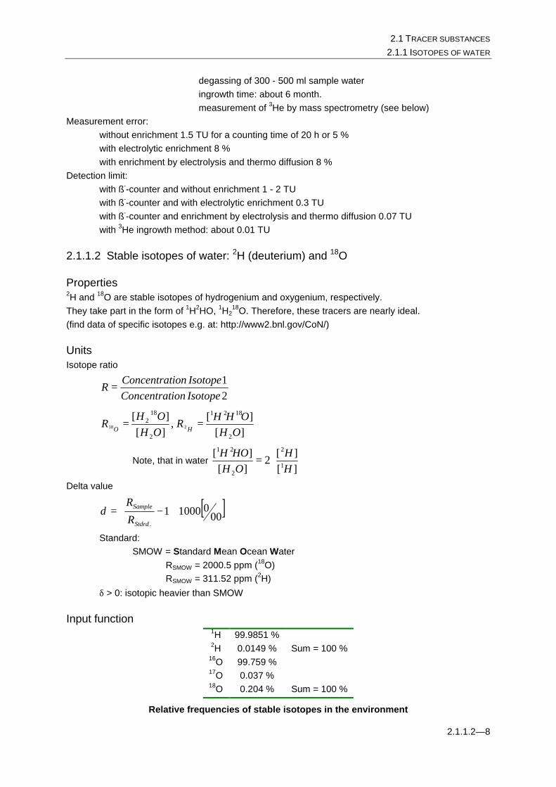
For the temperature dependence of the equilibrium separation factor the following equations hold:

052612.0248.7624844

)(ln 2 +−=TT

HDOeα

0020667.04156.01137

)(ln 218

2 +−=TT

OHeα

with: T in kelvin

Equilibrium separation factor of 2H and 18O and its temperature-dependence

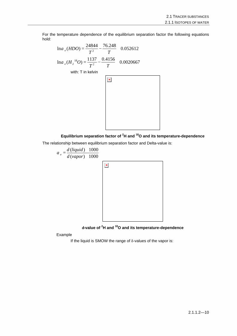
The relationship between equilibrium separation factor and Delta-value is:

1000)(1000)(

++

=vaporliquid

e δδ

α

δ-value of 2H and 18O and its temperature-dependence

Example

If the liquid is SMOW the range of δ-values of the vapor is:


2.1.1.2—11

δO-18(-20 °C) = -14 ‰ ... δO-18(+20 °C) = -9.7 ‰

δH-2(-20 °C) = -130 ‰ ... δH-2(+20 °C) = -78 ‰ Special case: Rayleigh condensation

Condensate will be removed instantly after condensation

Because 1>eα

)()( vaporliquid δδ >

( )( )

( )( ) 1000110001

..

⋅

−>⋅

−

vaporR

vaporR

liquidR

liquidR

Stdrd

Sample

Stdrd

Sample

( ) ( )vaporRliquidR SampleSample >

( ) ( )vaporOH

HDOliquid

OHHDO

22

>

Therefore: The system tries to increase the ration HDO/H2O in the liquid phase. If the condensate will be removed more and more HDO will leave the vapor.

Example: condensation in clouds where the condensate will be removed by raining.

δ-values decrease while clouds rain out. 2. Kinetic fractionation

In systems with incomplete vapor saturation: fractionation by different diffusion constants

(m

D1

∝ )

- no equilibrium - humidity < 100 %

proportional to deficit to full saturation = 0 for full saturation and = maximum for dry air

Example additional fractionation for half-saturated air and T = 20 °C is about

10 ‰ for both 2H and 18O Stable isotopes in the hydrologic circle

Water vapor above surface water is isotopic lighter then the water Continental effect:

Condensation and raining during the way from sea over the continent lead to decreasing isotope ratios

Temperature effect:

Temperature dependence of isotope fractionation leads to seasonal variation of isotope ratios in rain.

2H: about 2...3 ‰/°C Height effect:

As temperature varies with height fractionation varies with topographic level Seasonal effect:

As temperature varies with season fractionation varies with time


2.1.1.2—12

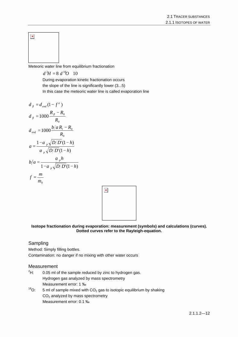
Meteoric water line from equilibrium fractionation

108 182 +⋅= OH δδ

During evaporation kinetic fractionation occurs the slope of the line is significantly lower (3...5) In this case the meteoric water line is called evaporation line

0

0

0

0

0

)1('1

)1('

)1('1

1000

1000

)1(

mm

f

hDD

hab

hDD

hDDa

RRRab

R

RR

f

p

p

p

p

lend

flfl

endfl

=

−−=

−

−−=

−=

−=

−=

α

α

α

α

δ

δ

δδ α

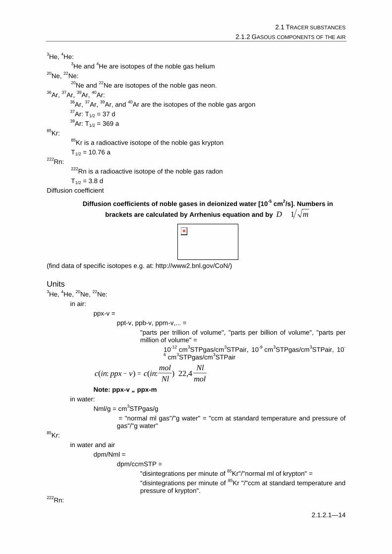
Isotope fractionation during evaporation: measurement (symbols) and calculations (curves). Dotted curves refer to the Rayleigh-equation.

Sampling Method: Simply filling bottles. Contamination: no danger if no mixing with other water occurs

Measurement 2H: 0.05 ml of the sample reduced by zinc to hydrogen gas. Hydrogen gas analyzed by mass spectrometry Measurement error: 1 ‰ 18O: 5 ml of sample mixed with CO2 gas to isotopic equilibrium by shaking CO2 analyzed by mass spectrometry Measurement error: 0.1 ‰


2.1.2.1—13

Excursion: Mass spectrometry

Principle of mass spectrometry

In the magnetic field charged particle are moving along a circular path Two forces: Lorentz-force FL:

×=

→→→

BvqFL

with: q = electric charge of the particle v = particle velocity B = magnetic field strength

and centrifugal force

rmv

Fz

2

=

with: m = mass of the particle r = radius of the circular path

On a circular path these forces must be equal

Lz FF =

This leads to

qBmv

r =

The kinetic energy of the particles origins from acceleration

2

21

mvqU =

with: U = acceleration voltage

And therefore:

qmU

Br

21=

This equation gives a possibility to separate isotopes. However, note that r depends on m/q, not m!

2.1.2 Gasous components of the air

2.1.2.1 Noble gases

Properties

2.1 TRACER SUBSTANCES 2.1.2 GASOUS COMPONENTS OF THE AIR

2.1.2.1—14

3He, 4He: 3He and 4He are isotopes of the noble gas helium

20Ne, 22Ne: 20Ne and 22Ne are isotopes of the noble gas neon.

36Ar, 37Ar, 39Ar, 40Ar: 36Ar, 37Ar, 39Ar, and 40Ar are the isotopes of the noble gas argon 37Ar: T1/2 = 37 d 39Ar: T1/2 = 369 a

85Kr: 85Kr is a radioactive isotope of the noble gas krypton T1/2 = 10.76 a

222Rn: 222Rn is a radioactive isotope of the noble gas radon T1/2 = 3.8 d

Diffusion coefficient

Diffusion coefficients of noble gases in deionized water [10-5 cm2/s]. Numbers in

brackets are calculated by Arrhenius equation and by mD 1∝

(find data of specific isotopes e.g. at: http://www2.bnl.gov/CoN/)

Units 3He, 4He, 20Ne, 22Ne:

in air: ppx-v =

ppt-v, ppb-v, ppm-v,... = "parts per trillion of volume", "parts per billion of volume", "parts per million of volume" =

10-12 cm3STPgas/cm3STPair, 10-9 cm3STPgas/cm3STPair, 10-

6 cm3STPgas/cm3STPair

c in ppx v c inmolNl

Nlmol

( : ) ( : ) ,− = ⋅ 22 4

Note: ppx-v ≠ ppx-m in water:

Nml/g = cm3STPgas/g = "normal ml gas"/"g water" = "ccm at standard temperature and pressure of gas"/"g water"

85Kr: in water and air

dpm/Nml = dpm/ccmSTP =

"disintegrations per minute of 85Kr"/"normal ml of krypton" = "disintegrations per minute of 85Kr "/"ccm at standard temperature and pressure of krypton".

222Rn:


2.1.2.1—15

in air dpm/l =

"disintegrations per minute of 222Rn"/" l of water" =

Input function Sources for noble gases in groundwater

- atmosphere: (3He/4He)air = 1.384·10-6

Volumetric composition of dry air

Isotopic composition of dry air

- excess air (see chapter 2.4): (3He/4He)air = 1.384·10-6 - in situ production of 4He by radioactive decay in the subsurface and 3He production by

6Li(n,α)3H→3He with thermic neutrons from (α,n)-reactions with light elements (Na, Mg and Al): (3He/4He)air = 10-9 ... 10-7. 4He accumulation rate from in situ production:

effThU

OH

rockisHe

nn

cct

c −⋅

⋅

⋅+⋅

⋅Λ=∂

∂−− 1

aµgHeSTPcm

1088.2aµg

HeSTPcm1019.1

4314

4313,

2

4

ρρ

with:

cU, Th = actual rock concentration of uran and thorium [µg/g]

ρrock ≈ 2.6 g/cm3 n = porosity neff = effective porosity

Λ = ratio of 4Heis amount in the pores to total amount of produced 4Heis ≈ 1 (recoil)

Example:


2.1.2.1—16

for U = 2 ppm, Th = 9 ppm and n = 20 % a time of about 10000 a is needed to produce the concentration equal to the equilibrium concentration from solution of atmospheric helium

- crust helium = helium produced in the subsurface beyond the aquifer and transported by diffusion into the groundwater: (3He/4He)crust = 10-9 ... 10-7

- helium from the upper mantle is a mixture of primordial and crust helium: (3He/4He)air = 1.1 ... 1.4·10-5

85Kr:

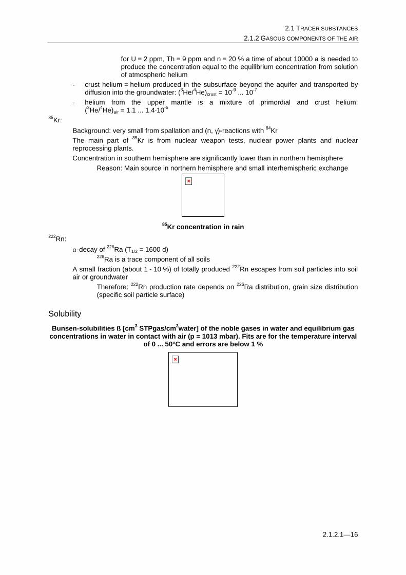
Background: very small from spallation and (n, γ)-reactions with 84Kr The main part of 85Kr is from nuclear weapon tests, nuclear power plants and nuclear reprocessing plants. Concentration in southern hemisphere are significantly lower than in northern hemisphere

Reason: Main source in northern hemisphere and small interhemispheric exchange

85Kr concentration in rain

222Rn:

α-decay of 226Ra (T1/2 = 1600 d) 226Ra is a trace component of all soils

A small fraction (about 1 - 10 %) of totally produced 222Rn escapes from soil particles into soil air or groundwater

Therefore: 222Rn production rate depends on 226Ra distribution, grain size distribution (specific soil particle surface)

Solubility

Bunsen-solubilities ß [cm3 STPgas/cm3water] of the noble gases in water and equilibrium gas concentrations in water in contact with air (p = 1013 mbar). Fits are for the temperature interval

of 0 ... 50°C and errors are below 1 %


2.1.2.1—17

Bunsen-solubilities ß [cm3 STPgas/cm3water] of the noble gases in water and equilibrium gas concentrations in water in contact with air (p = 1013 mbar).

Sampling Method:

Sampling with diving pumps for all gasous tracer in order to prevent degassing Flushing copper tubes and cold-pressure welding while flushing Remove bubbles by shaking and beating the tube

Sample container for noble gas analyses of groundwater analyses

Contamination: Contact with ambient air must be prevented (very important)

Taking groundwater samples for noble gas analyses in field 85Kr:

200 l of groundwater in stainless steel or polyethylen tanks. So much is needed in order to get a measurable signal.

222Rn: in pre-evacuated glass flasks or air-bags made of plastic-covered aluminium foil

Contamination: Contact with ambient air must be prevented

Measurement Noble gases:

gas extraction by stirring and shaking separation of noble gases by stepwise heating of adsorption trap


2.1.2.1—18

separation and detection of noble gas isotopes in a mass spectrometer Reproducibility: 2 ... 4 %

37Ar, 39Ar: separation of argon by gas chromatography Measurement by proportional counter

85Kr: Sample preparation:

Extraction of dissolved krypton by stripping with helium Accumulation of krypton at cryo trap Separation of krypton by gas chromatography

Sample preparation for 85Kr analysis of water

Measurement: Measurement of krypton by thermal conductivity detector Measurement of 85Kr by proportional counter

Measurement system for 85Kr analysis of water

Detection limit: 1,5 dpm/ccmSTPKr in water 222Rn:

Injection of 100 ml sample gas will be injected into ionization chamber filled with 1.5 l argon activity will be measured in slow-pulse ionization chamber Reproducibility: about 5 %


2.1.2.2—19

2.1.2.2 CFC's: Chlorofluorocarbons

Properties CFC-11 (CCl3F), CFC-12 (CCl2F2), CFC-113 (C2Cl3F3) no colour, no smell, chemical nearly inert Mainly used as propellent, refrigerant, solvent Strong greenhouse gases and ozone depletion Atmospheric lifetimes:

44 a (CFC-11) 180 a (CFC-12) 85 a (CFC-113)

Nomenclature for CFC's: CFC-XY methane related: methane = CH4

X = H atoms + 1 Y = F atoms

CFC-XYZ: X = C atoms - 1 Y = H atoms + 1 Z = F atoms

Example: CFC-113: 2 C atoms, 0 H atoms, 3 F atoms = C2F3Cl3

CFC-12: methane related, 0 H atoms, 2 F atoms = CCl2F2 In groundwater:

Inert with two restrictions: I. Adsorption II. Microbial degradation on anaerobic conditions

Diffusion coefficients:

RTmole

J

CFC es

cmD

200002

11 034.0−

− =

RTmole

J

CFC es

cmD

205002

12 041.0−

− =

Excursion: Retardation by adsorption Adsorption: chemical bond at mineral surfaces

Three types: I. bound without chemical reaction ("sorption/desorption") II. bound with reversible chemical reaction III. bound with irreversible chemical reaction (example: boron on clay minerals)

I. + II.: kationic tracer are more sorptive then neutral or anionic tracer, because matrix surface is charged negatively


2.1.2.2—20

Define: retardation factor R

T

w

uu

R =

with: uW = distance velocity of the water

uT = distance velocity of the tracer Define: distribution coefficient Kd

12 / CCK d = with:

C2 = concentration of adsorbed part of the tracer C1 = concentration of the water dissolved part of the tracer

For the distribution coeffient the following empirical relationship holds:

OCOCD KfK =

( ) ( ) bSaKOC +−= log2/log

Relation between retardation factor and distribution coefficient for

nKR df /1 ⋅+= γ

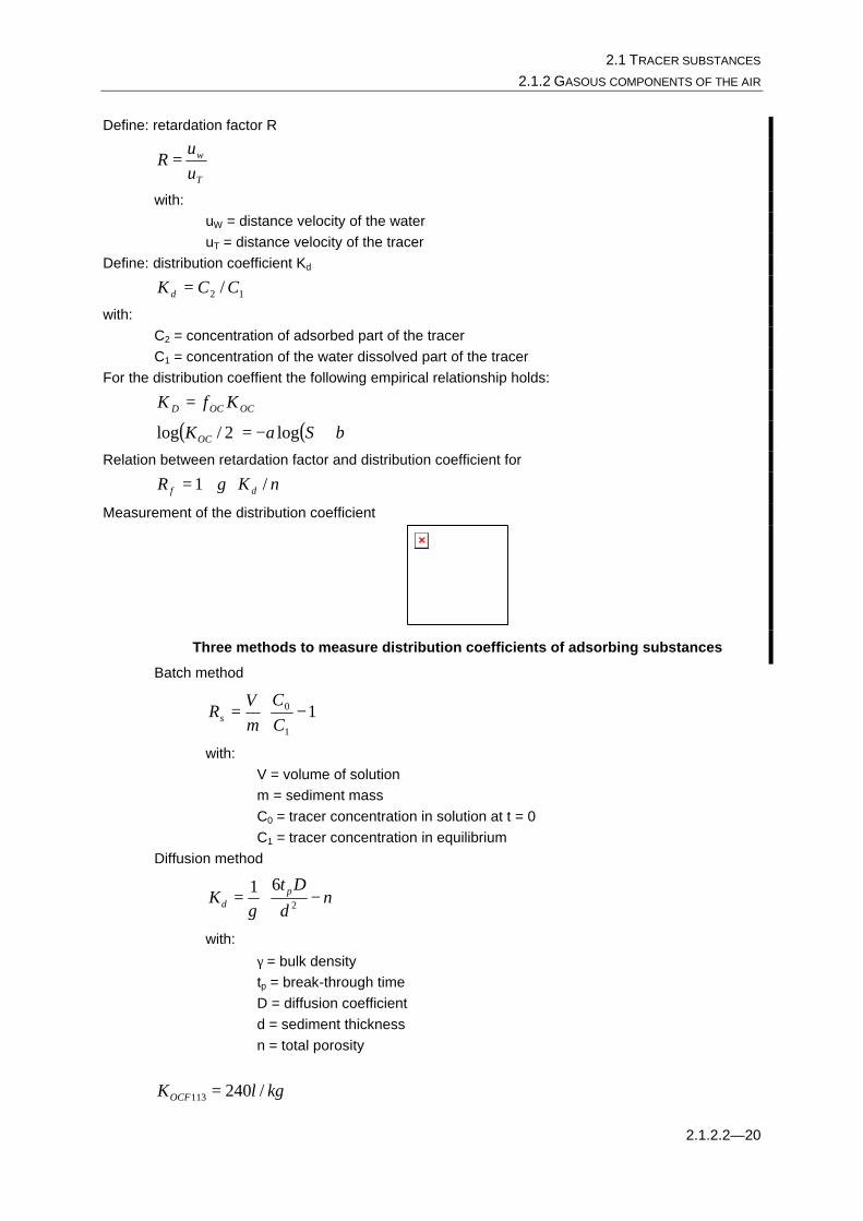
Measurement of the distribution coefficient

Three methods to measure distribution coefficients of adsorbing substances

Batch method

−= 1

1

0

CC

mV

Rs

with: V = volume of solution m = sediment mass C0 = tracer concentration in solution at t = 0 C1 = tracer concentration in equilibrium

Diffusion method

−= n

dDt

K pd 2

61γ

with:

γ = bulk density tp = break-through time D = diffusion coefficient d = sediment thickness n = total porosity

kglKOCF /240113 =


2.1.2.2—21

kglKOCF /10011 =

kglKOCF /27012 =

( ) ( ) dKcK OWOC += log2/log

kglKOCF /1400113 =

kglKOCF /24011 =

kglKOCF /14012 =

Microbial degradation on anaerobic conditions CFC can be degraded under anaerobic conditions.

Measured degradation rates lay within

0,05 - 2,3·104 pmol/(l·a) for CFC-12 0,4 - 3·105 pmol/(l·a) for CFC-11

The ratio of degradation rates seems to be constant = 9 ± 2

Units in air

ppx-v = ppt-v, ppb-v, ppm-v,... =

"parts per trillion of volume", "parts per billion of volume", "parts per million of volume" =




Nlmol

( : ) ( : ) ,− = ⋅ 22 4

Note: ppx-v ≠ ppx-m in water

fmol/l = 10-15 mol/l pmol/l = 10-12 mol/l

Input function Background:

Not known. Very low. Concentration in maritime air:

Input function of CFC-11, CFC-12 and CFC-113. Concentration data of maritime air from a global measurement program and emission data

Data is measured at maritime stations and calculated from emission data.


2.1.2.2—22

More and actual data find at http://cdiac.esd.ornl.gov/ndps/alegage.html.

Reconstruction of CFC-113 input function from emission data and concentration measurements of maritime air

Regional excess: In general the concentrations of CFC's in continental air are higher then in maritime air

Reason: These tracer will be emitted in continental air.

Define regional excess δ by

100C

0,

0 ⋅−

=L

LL

CC

δ (in%)

with: CL = concentration in the field area under investigation CL,0 = concentration in maritime air (at the same time)

Time serie of regional CFC-11 and CFC-12 excess as 222Rn concentrations in Heidelberg air, Germany. Strong peaks indicate local emissions. Here, 222Rn can serve as a tracer for

continental air.

Calculation of regional excess in former times by

( ) ( ) ( )( )timesamplingtE

tEtimesamplingtt

=== δδ

with: E = emission rate

Frequency distribution of the continental CFC-11 and CFC-12 excess for urban ("Heidelberg"), rural ("Wachenheim"), low mountain range ("Schauinsland") and

alpine air ("Colle Gnifetti")

continental excess [%]

CFC-12 CFC-11


2.1.2.2—23

alpine 10 10 low mountain 10 23

rural 24 34 urban 62 125

Concentration in southern hemisphere are significantly lower than in northern hemisphere

Reason: Main source in northern hemisphere and small interhemispheric exchange

Solubility Define solubility α by

airwater cc α=

with: cwater, cair = tracer equilibrium concentrations in water and air, respectively

Solubility of CFC-113: Measurement and Fit

CFC-12 : α12 (T) = 0.203 exp(-T/T12), ][2OHliterSTPGasliter with T12 = 20.36°C

CFC-11 : α11 (T) = 0.831 exp(-T/T11), ][2OHliterSTPGasliter with T11 = 19.48°C

CFC-113: α113(T) = 0.273 exp(-T/T113), ][2OHliterSTPGasliter

with T113 = 16.4°C

with T = temperature in °C

Temperature-dependence of the solubilities of CFC-12, CFC-11 and CFC-113 in water

Sampling Method:

Several methods are used:


2.1.2.2—24

1. Filling 500 ml glas bottles in cans under water

Sampling for CFC-analysis in 500 ml glas bottles

2. Filling up copper tubes similar to noble gas samples (see chapter 2.1.2.1 on page 2.1.2.1—17)

3. Filling up 62 ml glas ampules

Field apparatus used to fill and seal glass ampules for CFC determinations without allowing the sample to come in contact with air.

Differences in these techniques when degassing occurs because of different pressure during sampling and depending whether gas bubbles will be analyzed (copper tubes) or will be lost (glas bottles)

Contamination: No fat no oil

because of possible interference in the measurement system No contact with ambient air No contact with PVC during stroage

because of adsorption effects Reduce contamination by flushing all used materials with sample water

Measurement Degassing of samples by stripping with Ar/CH4 mixture. Separation of CFC's by gas chromatography and detection by electrone capture detector (ECD)


2.1.2.3—25

Gas chromatograph for CFC analyses

Chromatogram of a freon measurement

Detection limit: about 10 fmol/l Reproducibility: 3 % (CFC-11), 4 % (CFC-12), 5 % (CFC-113)

2.1.2.3 SF6: Sulphurhexafluoride

Properties Chemical inert: no smell, no taste, no colour Extremely high cross section for thermical electrones. Used:

- in insulating switchgear - as cover gas in magnesium and aluminium production to prevent oxidation - in isolating windows - in leak searchers - medical purposes (blowing up of collapsed lungs) - as tracer gas in scientific application

Strong greenhouse gas Atmospheric lifetime: about 3200 a Diffusion coefficient in water

Diffusion coefficients of SF6 in water.

Temperature [°C] Diffusion coefficient [10-6 cm2/s] 5 5.91 10 7.3 15 8.85 20 10.6

Units in air

ppx-v = ppt-v, ppb-v, ppm-v,... =

"parts per trillion of volume", "parts per billion of volume", "parts per million of volume" =




Nlmol

( : ) ( : ) ,− = ⋅ 22 4

Note: ppx-v ≠ ppx-m in water

fmol/l = 10-15 mol/l pmol/l = 10-12 mol/l

Input function


2.1.2.3—26

There is a natural component of SF6 in the environment. A natural background is estimated to abut 0.001 - 0.01 ppt-v. Mechanism of natural production is still not clear. Concentration in maritime air will be measured since about 1975. Data is described by

( ) ctyearpptv

pptvtcCG ∆+−⋅+= − 23 9.196910628.42373.0)(

∆c is different for northern hemisphere (∆cNH), southern hemisphere (∆cSH) and global mean (∆cG)

pptvtyearpptv

cNH 95.221065.11 3 −⋅⋅=∆ −

pptvtyearpptv

cSH 856.210450.1 3 −⋅⋅=∆ −

pptvtyearpptv

cG 90.1210548.6 3 −⋅⋅=∆ −

Input function of SF6 in comparison with the input functions of CFC-11, CFC-12 and CFC-113. Concentration data of maritime air from a global measurement program and emission data

Concentration in southern hemisphere are significantly lower than in northern hemisphere Reason: Main source in northern hemisphere and small interhemispheric exchange

Regional excess: In general the concentrations of CFC's in continental air are higher then in maritime air

Reason: These tracer will be emitted in continental air.

Define regional excess δ by

100C

0,

0 ⋅−

=L

LL

CC

δ (in%)

with: CL = concentration in the field area under investigation CL,0 = concentration in maritime air (at the same time)

Calculation of regional excess in former times by

( ) ( ) ( )( )timesamplingtE

tEtimesamplingtt

=== δδ

with: E = emission rate

Solubility


2.1.2.3—27

Sampling Method:

500 ml glas bottle for SF6 analysis of water

Instructions: 1. Flushing and filling the bottle (B) 2. Flushing the capillary tube (C) 3. Transport and storage (D) 4. Headspace injection (B) 5. Headspace in equilibrium (C) 6. Sample injection (B)

Diffusive flow through capillary tube during storage: < 0.002fmol/d

Contamination:

Prevent contact with ambient air A single air bubble of volume VL in the sample of volume VW' will lead to a measured concentration cW

* of

2.1 TRACER SUBSTANCES 2.1.3 FURTHER SUBSTANCES

2.1.3.1—28

LW

LLWWW VV

VcVcc

++

=*

with: cW = true tracer concentration in water cL = tracer concentration in recent air.

Error estimation by contact with air. For the calculation it is assumed that an air bubble occurs in the sample (cL = 5 pptv, VW = 550 ml). Dependence of measured tracer

concentration on real tracer concentration and volume of the air bubble can reach values up to 100 % of the true water concentration

Measurement

Gas chromatograph for SF6 analysis of water

Injection of a headspace of carrier gas. Gas extraction by 20 min shaking Separation of SF6 by gas chromatography.

Carrier gas: N2 Column material: molecular sieve (5 ?) Adsortion trap material: Porapak-Q Column temperature: 65 °C Detector temperature: 330 °C

Detection by electrone capture detector Detection limit: 0.015 fmol = 15 amol = nine million molecules! Reproducibility: about 3 %

2.1.3 Further substances

2.1.3.1 Carbon-14 (14C)

Properties 14C is the radioactive isotope of carbon T1/2 = 5730 ± 30 a


2.1.3.1—29

14C will be introduced in the groundwater as part of C-compounds (e.g.CO2, CH4). Because these compounds are highly reactive, 14C must be considered as a reactive tracer (compare chapter 2.5.1.1)! (find data of specific isotopes e.g. at: http://www2.bnl.gov/CoN/)

Units Delta-notation similar to that of the stable isotopes of water

dardS

dardSSample

R

RR

tan

tan−=δ

pmc: Percent modern carbon with: 100 pmc

= "one hundred percent of modern carbon" = atmospheric 14C concentration 1950

Concentrations above 100 pmc result from bomb-14C

Input function 14C will be produced by thermic neutrons of cosmic rays

)( 1414 pCnN +→+

214

214 COOC →+

14CO2 will be distributed homogenously over the atmosphere Production rate and radioactive decay lead to a 14C equilibrium concentration 14C/12C = 1.18·10-12 coresponding to 14C-activity of 13.56 dpm

Atmospheric 14C level for the last 12000 years

Reasons for the long-time decrease of 14C - Higher production rate in the past because of lower earth magnetic dipole moment and therefore

higher cosmic ray intensity - Variation of the carbon cycle because of climatic variations and release of old 14C-free carbon - Variations of ocean circulation and release of old 14C-free carbon Reasons for the short-time variations of 14C - sun activity variations - climatic variations ("De Vries effect")

Concentration of 14C in the atmosphere for the last century. Nuclear weapon tests produce a peak in the last 50 years. Before that, concentrations are slightly decreasing because of

burning of fossil oil and coal with 14C = 0

2.1 TRACER SUBSTANCES 2.1.3 FURTHER SUBSTANCES

2.1.3.1—30

Calibration curves to correct 14C ages for long-time decreases and short-time variations, estimated by absolute tree-ring age dating.

Zoom-In of the figure before with experimental data. Calibration curve is not neessary unique

Sampling Method:

At least two methods exist in the literature 1. circulation method:

Circulation in avacuum tight circulation system Injection of HCl in 60 l sample water Free CO2 will be absorbed in a NaOH bottle

2. precipitation method: Injection of BaCl into 60 l sample water

this leads to BaCO3 → precipitation → decantation 3. ion exchange method

Contamination: Prevent contact with the atmosphere

Equibment for 14C sampling

Measurement


2.2.3.1—31

Injection of HCl into sample 192 ml of free CO2 gas will be analyzed by low-level counting

Measurement for 14C analysis

Detection limit: 0.5 pmc for low-level counting Measurement error: 0.4 pmc for low-level counting

2.2 Getting samples

2.2.1 Overview Mixing by sampling can cause serious interpretation errors - PREVENT MIXING! Try to get vertical concentrations profiles

2.2.2 Samples from springs

Schematic vertical cross section of a spring

In springs, mixing cannot be prevented. Vertical concentration profiles are not possible.

2.2.3 Samples from groundwater wells

2.2.3.1 Multilevel wells

Individual wells and nests. (a) separate short-screened wells sunk to each sampling depth. (b) Three piezometers nested in one drill hole.

2.2 GETTING SAMPLES 2.2.3 SAMPLES FROM GROUNDWATER WELLS

2.2.3.2—32

Schematic scetch of amultilevel well. a. single pump is running, b. all pumps are running

Catchment area of pumps in a multilevel well indicated by pathlines while all pumps are running

Advantage: Multilevel wells are easy to use and lead to exact depth. Disadvantage: not flexible and expensive

Example: Tracer profiles from multilevel well samples

Concentration profiles of CFC-11, CFC-12, CFC-113 and 3H from multiwell sampling. The profiles show the input function of these tracers, see chapter 2.1.1.1 and 2.1.2.2.

2.2.3.2 Vertical concentration profiles from long-screened wells

A typical long-screened well

Bailer

Depth samplers. (a) Bailer is lowered to sampling depth and recovered. (b) Alternative valving arrangements for bailers.

Variation of this technique: pumping with very low rate at the specific depth Disadvantage:

Flow through the borehole before and during sampling lead to concentration profiles inside the borhehole which differ from concentration profiles in the aquifer


2.2.3.2—33

Packer installations

Schematic diagram of a double packer system.

Main disadvantage: possibility of short circuit through the filter gravel

Short-circuit through the filter gravel for packer installations

Packer installations in open holes:

Dedicated multi-level system for a single well, with packers separating the sampling intervals.

Baffle system

Baffle system, with main pump inducing inflow to well, and sampling pump collecting water from inside the baffle

Separation of horizontal inflow. Disadvantage:

Possibility of short-circuit through filter gravel

Multi-port sock sampler

Concept of a multi-port sock sampler.

Disadvantage: specific influx distribution must be known for estimation of catchment area: sampling depth is not necessary depth of the port.

Separation Pumping Technique

2.2 GETTING SAMPLES 2.2.3 SAMPLES FROM GROUNDWATER WELLS

2.2.3.2—34

Separation Pumping Technique, with sampling pump positioned at water divide between flow to the top and bottom pumps

Creation of a water divide with horizontal inflow and sampling from this depth. This technique stems from scavenge pumping.

Dual Pumping Technique

Water table

Upper pump

borehole filter

Flowmeter

Valve

Production pipe

WinchNotebook-PC

Flowmeter

To second sampling branch

Tap for sampling

water divide z(()

Lower pump

First sampling branch

d.q(.)dQ(.) = q(.)2BRd>

. = 0

. = m

Concept of the Dual Pumping Technique.

The pumping ratio is

tot

b

tb

bb Q

QQQ

Q=

+=γ ; [ ]10 b ≤≤ γ

with:


2.2.3.2—35

Qb = pump rate at the bottom pump Qt = pump rate at the top pump.

The measured concentration at the bottom pump Cb is

( )( )

( )

( )

( )( )

∫

∫=

b

0

0bb

Rd2q

Rd2

γ

γ

ζπζ

ζπζζγ z

z

qcC

b

with:

ζ = depth, running from ζ = 0 at the lower end of the borehole to ζ = m at the upper end of the borehole

c(ζ) = concentration profile in the aquifer

q(ζ) = specific influx distribution in the aquifer.

z(γb) = depth of the water divide, dependent on the pumping ratio γb For the pumping rate of the bottom pump Qb we receive

( )( )

∫ ==b

0bbtotRd2

γ

γζπζz

QQq

so that

( )

( )

( ) ( )

RQ

qc

C

z

πγ

ζζζγ

γ

2

d

btot

0bb

b

∫= .

Isolating the integral leads to

( ) ( ) ( )( )

∫=b

0bbb

tot d2

γ

ζζζγγπ

z

qcCR

Q

By derivation with respect to γb on both sides of the equation (chain rule:

bbb

b ddz

zfdzd

zfd

dγ

γγγ

))(())(( = !) we receive

( ) ( ) ( )( ) ( )( ) ( )b

bbb

totb

b

bbb

tot

ddz

2ddC

2 γγ

γγπ

γγ

γγ

πzqzc

RQ

CR

Qb =+

from which the concentration profile in the aquifer can be isolated

( )( )( ) ( )

( )( ) ( )b

bb

totb

b

bbb

tot

b

ddz

2ddC

2

γγ

γ

πγ

γγ

γπ

γzq

RQ

CR

Q

zcb +

=

The denominator we receive by derivation the equation for the pumping rate of the bottom pump Qb with respect to γb:

( )( ) ( )R

Qzq

πγγ

γ2d

dz tot

b

bb =

And so, as the most important equation for the Dual Pumping Technique we find

( )( ) ( ) ( )b

b

bbbb d

dCγ

γγ

γγ += bCzc .

2.2 GETTING SAMPLES 2.2.4 GAS SAMPLES

2.2.3.2—36

Dual pumping technique in field

Comparison of vertical 3H profiles, determined by DPT and multilevel well

2.2.4 Gas samples In general, gas samples are taken the same way as water samples


2.2.3.2—37

Schematic scetch of an equibment for sampling ground air to analyze SF6 and 222Rn

2.3 Transport through unsaturated zone

Path of a tracer molecule from injection into the system to the sample point.

Two processes can be simplified: Gasous tracer will be transported mainly by diffusion Water-beared tracer will be transported mainly by advection Rule of thumb:

Diffusive transport is several orders of magnitude faster then advective transport!

2.3.1 Transport of gasous tracer Main transport process for gasous tracer through the unsaturated zone is diffusion

Fick's second law

cDtc

∆=∂∂

with: c = tracer concentration t = time

∆ = Laplace operator = 2

2

2

2

2

2

2

2

zzyx ∂∂

=∂∂

+∂∂

+∂∂

=∆

D = effective diffusion coeffient

kFn

DD−

= 0

with: D0 = diffusion coefficient in air n = total porosity F = soil moisture content k = tortuosity

k describes the higher diffusion resistance due to variation of diffusion cross-section in the soil by soil-grains and water-filled capillary regions

For 222Rn the transport equation changes to

cQcDtc

λ−+∆=∂∂

2.3 TRANSPORT THROUGH UNSATURATED ZONE 2.3.2 TRANSPORT OF DISSOLVED TRACER

2.2.3.2—38

with: Q = source strength of 222Rn normalized to unit soil volume depending on 226Ra distribution, grain size distribution (specific soil particle surface)

λ = decay constant of 222Rn = 2.1⋅10-6 1/s For homogenous D and Q this equation will be solved by

)1()( zz

eczc−

∞ −=

if border conditions

0)0( ==zc and 0=

∂∂

∞→zzc

are assumed, with:

λQ

c =∞

λDz =

This equation can be used to determine effective diffusion parameters of natural soils.

222Rn profile in a sandy unsaturated zone. From this profile an effective diffusion coefficient of D = 6.1⋅10-8 m2/s can be estimated

The diffusive transport through the unsaturated zone retards the transport of gasous tracer from the atmosphere to the groundwater table

Concentration of CFC-113 in ground air and its equilibrium water concentration at various depths - measurements and calculations

2.3.2 Transport of dissolved tracer Description of advective flow through the unsaturated zone

Richards equation

Darcy equation with ( )( ) 1+

=θ

ψθ

dzd

vk f

u

With the Richards equation the transport of the tracer can be calculated by


2.2.3.2—39

( ) ( ) ( ) QcDcvtc

+∇Θ∇=∇+∂Θ∂ rrr

with:

Θ = water content c = tracer concentration t = time

∂∂

∂∂

∂∂

=∇zyx

,, = "Nabla operator"

v = distance velocity D = dispersion coefficient Q = sinks/sources

Assumptions for long-time tracer transport: - no dispersion - no sinks/sources - water content is constant - no horizontal components of flow

For these assumptions the transport velocity is constant

Θ=

Rv

with: R = groundwater recharge

Neglection of advective transport through the unsaturated zone can lead to significant different concentration distributions, e.g. for tritium

2.4 EXCESS AIR IN GROUNDWATER 2.3.2 TRANSPORT OF DISSOLVED TRACER

2.2.3.2—40

XSteinbruchX GW 5

X GW 4X GW 3

X

X GWMII

X GW 2

X TBr. 2 +1

X GWMIIIX GWMV

X GWMAutob.

X GWMIV

X HBr.C

X GWMI

500 1000 1500 2000 2500x [m]

500

1000

1500

2000

2500

3000

3500

y

[ m

]

5.00

7.00

9.00

11.00

13.00

15.00

17.00

19.00

21.00

[TU]

X SteinbruchX GW 5X GW 4

X GW 3

X

X GWM II

X GW 2

X TBr. 2 + 1

X GWM IIIX GWM V

X GWM Autob.

X GWM IV

X HBr. C

X GWM I

500 1000 1500 2000 2500

x [m]

500

1000

1500

2000

2500

3000

3500

y [m

]

10.00

15.00

20.00

25.00

30.00

35.00

40.00

45.00

50.00

55.00

60.00

65.00

[TU]

Calculated 3H distributions in two models where in the right one 3H transport through the unsaturated zone is considered while in the left one it is not. The residence time of water is

about 3 a in the saturated zone and in the range of 0 a to 30 a in the unsaturated zone.

2.4 Excess air in groundwater Define:

Excess air in groundwater = air concentration in groundwater above equilibrium Mainly caused by:

groundwater table variation

⇒ dead-end pores filled with air under hydrostatic pressure

⇒ dissolution of air in water. Excess air in groundwater is an error source for gasous age dating tracer. Quantification is possible by the isotopes of neon because

- neon concentration is constant over time, - atmosphere is the only source for neon in groundwater, - solubility of neon is low, - temperature-dependency of solubility is low. Quantification of excess air by neon isotopes is possible by the following equations:

cNe in water = αNe in watercNe in air + cNe from excess air

cNe from excess air = cNe in water - αNe in watercNe in air cexcess air in water = cNe from excess air*1/RNe

air

cexcess air in water = (cNe in water - αNe in watercNe in air)*1/RNeair

For quantification the recharge temperature must be known Therefore, an iterative technique is used to determine recharge temperatures and excess air in groundwater

(1) Measurement of noble gas concentrations (except helium because of other sources than the atmosphere)

(2) Recharge temperature calculation by measured concentrations and solubilities (3) Are calculated recharge temperatures equal for all noble gases?

(4) If yes: STOP (5) If no:

(6) Theoretic neon concentration calculation by estimated recharge temperature


2.2.3.2—41

(7) Interprete the difference between calculated and measured concentration by excess air and calculate the amount of excess air in the sample

(8) Correct the measured values of noble gases for excess air (9) GOTO (1)

For each tracer the following equation holds:

ctracer in water = αTracerctracer in air + cexcess air in waterctracer in air

ctracer in water = αTracerctracer in air(1 + cexcess air in water/αtracer)

The excess air correction factor (1 + cexcess air in water/αtracer) depends on solubility

2.5 Interpretation of environmental tracer measurements What can we expect from measurement of environmental tracer?

Age dating transport velocity groundwater recharge sanitation duration

Transferfunction

f dd

( )τ ττ τ τ

=+Water in a sample with an age beween and

Total water in the sample

Therefore:

f d( )τ τ =∞

∫ 10

In this case the measured tracer concentration can be calculated by

τττ dftctc intracerout )()()(0

, ∫∞

−=

with: t = sampling time and the mean residence time can be determined by

ττττ df )(0∫∞

=

recharge area recharge temperature

2.5.1 Analytic models

2.5 INTERPRETATION OF ENVIRONMENTAL TRACER MEASUREMENTS 2.5.1 ANALYTIC MODELS

2.5.1.1—42

2.5.1.1 Piston-Flow-Model

Scetch of a Piston-Flow-Model

Transfer function of the piston flow model

( ) ( )ττδτ −=f

with:

δ = Dirac delta function which is defined by:

( )

( )∫∞

=−

≠=−

0

1

,0

τττδ

ττττδ

d

For piston flow models the age of a sample can easily read from the input function, eventually corrected for radioactive decay or other sinks/sources. The piston flow model applicable for vertical profiles

(a) Depth profiles of 3He in a shallow aquifer at Liedern/Bocholt, Germany, (b) the same as (a) for 3H and 3H + 3He, (c) the same as (a) for the 3H/3He age

Groundwater recharge estimation in a Coast Aquifer, Northern Germany

Special case: "Conventional 14C ages" Define "conventional 14C age" by

assumptions closed system piston-flow model start concentration c0 = 100 pmc

Then

=

pmcc

t100

ln1λ

is called "conventional 14C age".


2.5.1.2—43

The "conventional 14C age" is simply another scale for the measured concentration. The significance of it is very low, because - in general, there is a mixture of ages in a sample so that the piston-flow model is not valid - c0 = 100 pmc in groundwater is not necessary true, because CO2 can dissolve fossile lime

with 14C = 0 14C-free lime dissolution in a closed system (stoichiometry: one CaCO3 dissoluted by one CO2): c0 = 50 pmc Reality: c0 = 50 ... 100 pmc

Correction models for the c0 assumption of "conventional 14C ages" - c0 = 85 pmc; that is the average from about 100 shallow

groundwater samples - Assumption: HCO3 in groundwater stems to equal parts from CO2

and lime.

[ ] [ ]( ) [ ][ ] [ ]−

−−

+

++=

32

lim3320

5.05.02

HCOCO

AHCOAHCOCOc eCO

with: ACO2 = ratio of 14C to 12C in CO2 - Atmospheric 14C is not a constant with time - further chemical reactions during transport in the aquifer, e.g. bacterial production of CO2 by sulfate reduction.

However, the "conventional 14C age" is widely used and because of the name many user interprete the "conventional 14C age" as the real age!

2.5.1.2 Exponential Model Transfer function for the exponential model

( ) ( )τττ

τ /exp1

−=f

Realsations of an exponential model: Vogel model

Assume semi-infinite 2D vertical aquifer with a constant recharge 0=∂∂

xvz .

Because 0=vrotr

we receive

0=∂∂

zvx

Because 0=vdivr

we can conclude that

.constzvz =

∂∂

and therefore that

2.. constzconstvz +⋅=

With the border conditions 0)( == mzvz (aquiclude) and Nzvz == )0( with N = recharge we receive

mzm

NNzmN

vz−

=+⋅−=

Because 0=vdivr

the following equation holds:

mN

xvx =

∂∂


2.5.1.2—44

which will together with the border condition 0)0( ==xvx (water divide) lead

to

xmN

vx =

For a water particle we get therefore the differential equation

mzm

NNzmN

dtdz −

=+⋅−=

which will be solved by

( )

−=

− tmN

emtz 1

if border condition z(0) = 0 is assumed. To find the transfer function in a homogenous aquifer we can start with

( ) { dtNem

dzm

dttft

mN

tiontransformaiable

−==

11

var

A well in a homogenous horizontal 2D aquifer with a stationary catchment area is also a exponential aquifer.

3H output concentration for the exponential model for a sample time of 1998

For 3H no unique solution exists for age dating with the exponential model. This is a direct consequence of the shape of the input function.

Example

3H concentration in Funtenen Well at Meiringen, Switzerland. Parameter is the Mean Residence Time calculated with the exponential model


2.5.1.4—45

For a sine-shaped input function ( ) ( )( )τϖτ −=− tAtcin sin the cout function is also shaped but

damped by the factor 2)(1

1

τω+=f

Damping 2)(1

1

τω+=f of the output function for a sine input with

a12π

ϖ =

dependent of the mean residence time

2.5.1.3 Dispersion Model

Scetch of the Dispersion Model

Tranfer function of the Dispersion Model

( ) ( )

−−

=τ

τττ

ττ

πτ

PePe

f4

exp4

1 2

with: Pe = uL/D with:

u = distance velocity L = characteristic length D =

Transfer Function for the Dispersion Model with different parameter

2.5.1.4 Transfer function for 3H/3He dating Two age determination methods exist for 3H/3He dating:


2.5.1.5—46

The sample helium concentrion is given by an integral which can be splitted in two:

( ) ( )( ) τττ λτ detCfCinout

−∞

−−= ∫ 10

H,He, 33

( ) ( ) ( ) ( ) ττττττ λτ detCfdtCfinin

−∞∞

−−−= ∫∫0

H,0

H, 33 .

The second integral is the sample tritium concentration

( ) ( )H,

0H,He, 333 outinout

CdtCfC −−= ∫∞

τττ

which is also measured. Two equations for cout, 3He give a possibility to prove the choosed transfer function. Both evaluation equations must lead to the measured concentrations, otherwise the transfer function is surely not correct.

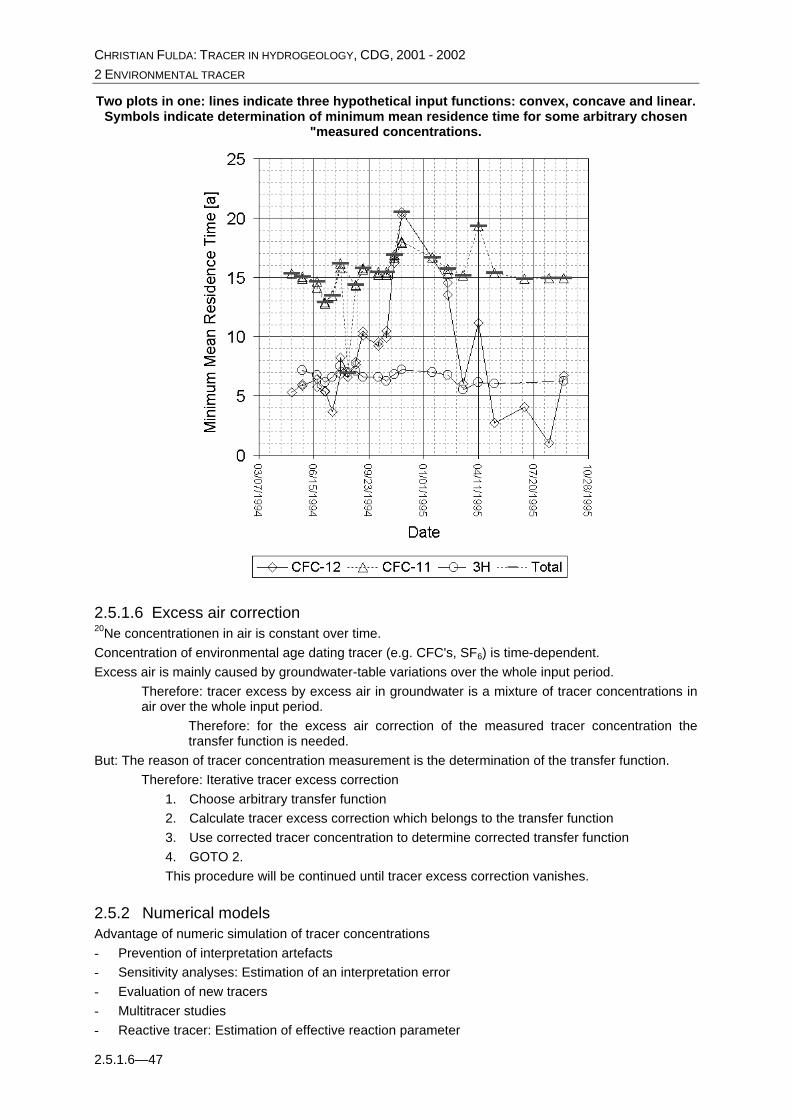
2.5.1.5 Minimum Mean Residence Time In praxis discretized equations for mean residence time determination are used:

Nfff ...1 21 ++=

with:

Nif i ≤≤≥ 1for 0

NinNininout cfcfcfc ,2,21,1 ...++=

NNfff ττττ ...2211 ++=

These equations cannot solved exactly because they are overdetermined. But the minimum mean residence time can be calculated exactly. Then we have an optimization proplems with constraints.


2.5.1.6—47

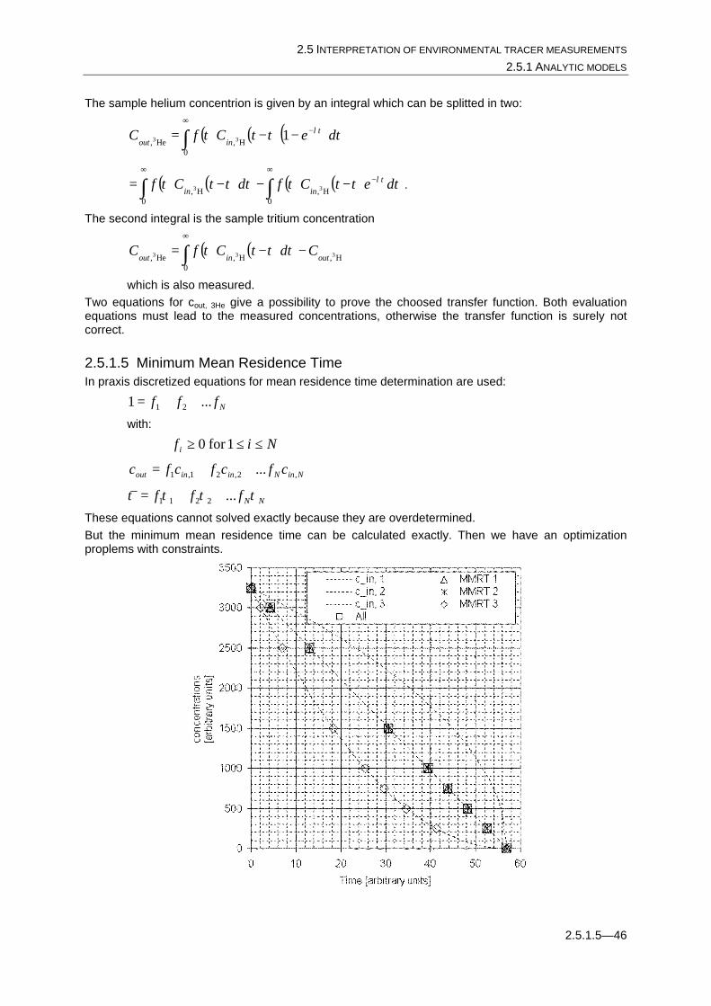
Two plots in one: lines indicate three hypothetical input functions: convex, concave and linear. Symbols indicate determination of minimum mean residence time for some arbitrary chosen

"measured concentrations.

2.5.1.6 Excess air correction 20Ne concentrationen in air is constant over time. Concentration of environmental age dating tracer (e.g. CFC's, SF6) is time-dependent. Excess air is mainly caused by groundwater-table variations over the whole input period.

Therefore: tracer excess by excess air in groundwater is a mixture of tracer concentrations in air over the whole input period.

Therefore: for the excess air correction of the measured tracer concentration the transfer function is needed.

But: The reason of tracer concentration measurement is the determination of the transfer function. Therefore: Iterative tracer excess correction

1. Choose arbitrary transfer function 2. Calculate tracer excess correction which belongs to the transfer function 3. Use corrected tracer concentration to determine corrected transfer function 4. GOTO 2. This procedure will be continued until tracer excess correction vanishes.

2.5.2 Numerical models Advantage of numeric simulation of tracer concentrations - Prevention of interpretation artefacts - Sensitivity analyses: Estimation of an interpretation error - Evaluation of new tracers - Multitracer studies - Reactive tracer: Estimation of effective reaction parameter

2.5 INTERPRETATION OF ENVIRONMENTAL TRACER MEASUREMENTS 2.5.2 NUMERICAL MODELS

2.5.2.2—48

Two methods: - Age dating and simulation of groundwater ages

Advantage: only pathline simulations are needed Disadvantage: samples from single depths are needed

- Simulation of tracer distributions Advantage: all measured concentrations can be used for model calibration Disadvantage: Simulations are cost- and time-consuming.

Example: determination of the transfer function for a hpothetical exponential model aquifer by numerical simulation.

2.5.2.1 Parameter variation

Example Spatial variable groundwater recharge for a hypothetical exponenttial model and the corresponding transfer function

Piecometric surface, capture area and transfer function for a hypothetical aquifer which is an ideal exponential model aquifer except for a variable groundwater recharge

2.5.2.2 Sensitivity analyses


2.5.2.3—49

Transfer function for the transport through saturated and unsaturated/saturated zone

2.5.2.3 Complex simulations Complex numerical simulation is the only possibility for consistent evaluation of tracer and other hydrogeological data. Example: estimation of catchment area of the mineral wells at Stuttgart, Germany, by means of stable isotopes and numerical simulations on a regional scale

Overview of the investigation area with sampling points

Complex transmissivity distribution estimated by geological information and pump test data

Scatter-diagram: Comparison of calculated and measured concentrations

3.1 TRACER SUBSTANCES 3.1.1 DYE

3.1.1.1—50

Recharge area of the mineral wells in Stuttgart, determined by stable isotopes and numerical simulations

2.5.2.4 Multitracer studies and estimation of reaction parameters

Multitracer study for a basalt aquifer in Germany. Upper row: gas tracer to calibrate transport simulation through saturated zone. Lower row, left: water-beared tracer to calibrate transport simulation through unsaturated zone. Lower row, right: reactive tracer to estimate effective

reaction parameters

3 Artificial tracer Properties of a good artificial tracer:

- absence or very low concentration in the environment - wide measurement concentration range, low detection limit - no influence on plants, animals and human beings - easy to solute in water - inert in groundwater - no influence on groundwater flow and transport - not too expensive

3.1 Tracer substances Note: all environmental tracers can be used as artificial tracers

3.1.1 Dye

3.1.1.1 Uranin

Properties Nomenclature:

CHRISTIAN FULDA: TRACER IN HYDROGEOLOGY, CDG, 2001 - 2002 3 ARTIFICIAL TRACER

3.1.1.1—51

sodium fluorescine sicomet

Chemical formula: C20H10O5Na2

Molar mass: 376.28 g/mole

Structure: For all fluorescines the structure is:

Structure of fluorescines. For explanation see next table

Solubility: more than 600 g/l (20 °C) Degradation of uranin by strong oxidants

Units g/m3 or similar units

Sampling Method: simply filling bottles Contamination:

Possibly by the operator himself Never inject and sample at the same day, with the same equibment and even the same clothes for uranin. Degradation of uranin by light

Destruction of a uranin solution (10 µg/l) by light in a brown and a transparent glass bottle

Adsorption very low.

Measurement Fluorometry

Maximum of extinction: 491 nm Second maximum of extinction: 322 nm Maximum of fluorescence: 512 nm Fluorescence of uranin solution depends on uranin concentration.

3.1 TRACER SUBSTANCES 3.1.2 IONS

3.1.1.2—52

Uranin calibration curve

Dependence of the uranin fluorescence intensity on pH

Correction by pH fluorescence calibration curves or: fix a constant pH value by injection of a

Stimulation and fluorescence intensities of uranin

Detection limit: about 10-9 g/l

3.1.1.2 Pyranin

Properties

Units

Sampling

Measurement

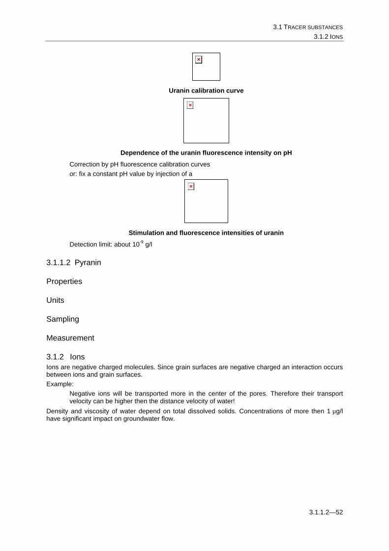
3.1.2 Ions Ions are negative charged molecules. Since grain surfaces are negative charged an interaction occurs between ions and grain surfaces. Example:

Negative ions will be transported more in the center of the pores. Therefore their transport velocity can be higher then the distance velocity of water!

Density and viscosity of water depend on total dissolved solids. Concentrations of more then 1 µg/l have significant impact on groundwater flow.


3.1.2.2—53

Density and dynamic viscosity of water depending on total dissolved solids.

3.1.2.1 NaCl

Properties Calculation of NaCl equivalent concentration from measurements of water resistivity ρ

)(1

5,21)(5,61

4000)(zCzT

ppmzCρ°+

=

with: T = temperature [°C]

Units

Sampling

Measurement

3.1.2.2 Bromide

3.2 Single-well methods

3.2.1 Vertical flow in groundwater wells induced by long filter screens

3.2 SINGLE-WELL METHODS 3.2.1 VERTICAL FLOW IN GROUNDWATER WELLS INDUCED BY LONG FILTER SCREENS

3.1.2.2—54


3.1.2.2—55

3.2.2 Dilution method Injection of a tracer into a borehole and measurement of its concentration decrease with time.

Shematic horizontal cross section of a borehole and the surrounding aquifer with flowlines

Experimental sutdy of the horizontal flow through a vertical borehole with and without filter gravel and dilution of a tracer inside the borehole

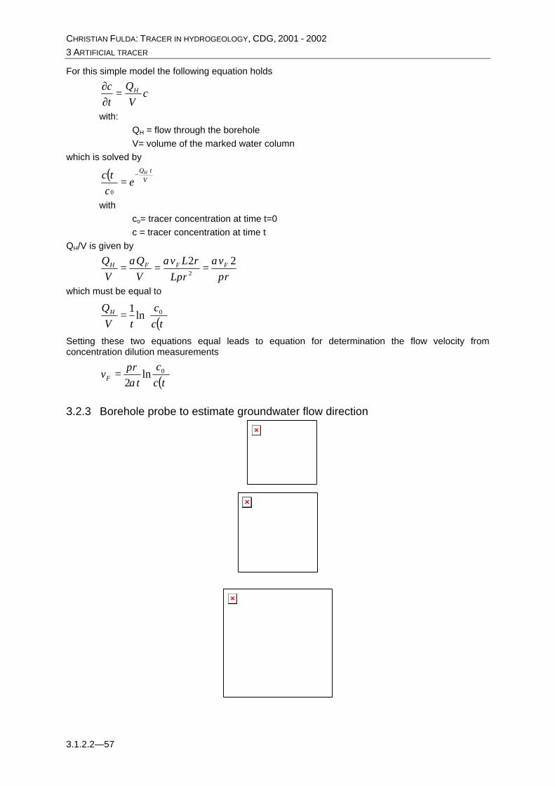
Horizontal flowlines in a borehole for different position of the screen slids

Screen slides in a filter casing are more or less plugged

Suitable part of screen in a monitoring well dirty segment of screen in a monitoring well, not suitable for measuring

The focusing effect of the borehole is described by the factor α:

FH QQ ⋅= α with:

3.2 SINGLE-WELL METHODS 3.2.2 DILUTION METHOD

3.1.2.2—56

QH = flow through the borehole QF = Darcy flow through the aquifer

In a homogenous aquifer without filter gravel, infinite permeability inside the borehole and no resistance from the filter screen

α = 2 In a homogenous aquifer without filter gravel, infinite permeability inside the borehole and finite permeability of the filter screen

−+

+

=2

2

1

1

2

2

111

4

rr

kk

rr f

α

with: k1 = permeability of the filter screen

kf = permeability of the aquifer r1 = inner radius of the filter tube r2 = outer radius of the filter tube

In a homogenous aquifer with filter gravel, infinite permeability inside the borehole and finite permeability of the filter screen

−

+

+

−+

−+

+

+

=2

3

22

3

1

1

22

3

22

3

1

2

2

2

1

1

22

2

1

21111

8

rr

rr

kk

rr

rr

kk

rr

kk

rr

kk ff

α

with:

k2 = permeability of the filter gravel r3 = radius of the borehole

Schematic model for evaluation of tracer dilution measurements


3.1.2.2—57

For this simple model the following equation holds

cV

Qtc H=

∂∂

with: QH = flow through the borehole V= volume of the marked water column

which is solved by

( ) VtQH

ectc ⋅

−=

0

with co= tracer concentration at time t=0 c = tracer concentration at time t

QH/V is given by

rv

rLrLv

VQ

VQ FFFH

πα

παα 22

2 ===

which must be equal to

( )

=

tcc

tVQH 0ln

1

Setting these two equations equal leads to equation for determination the flow velocity from concentration dilution measurements

( )tcc

tr

vF0ln

2απ

=

3.2.3 Borehole probe to estimate groundwater flow direction

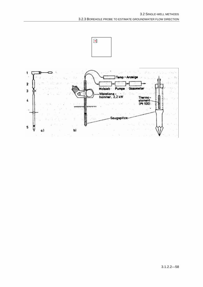
3.2 SINGLE-WELL METHODS 3.2.3 BOREHOLE PROBE TO ESTIMATE GROUNDWATER FLOW DIRECTION

3.1.2.2—58


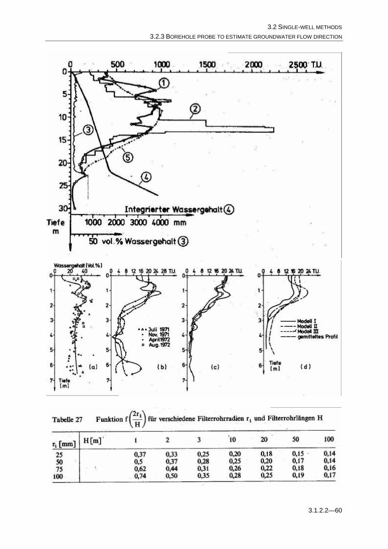
3.1.2.2—59

3.2 SINGLE-WELL METHODS 3.2.3 BOREHOLE PROBE TO ESTIMATE GROUNDWATER FLOW DIRECTION

3.1.2.2—60


3.1.2.2—61

Geoelectric installations to determine local flow and transport parameters by salt injection and geoelectric determinations of tracer cloud movement

3.3 More-well methods

Piecometric surface for a limestone aquifer, South Germany

3.3 MORE-WELL METHODS 3.2.3 BOREHOLE PROBE TO ESTIMATE GROUNDWATER FLOW DIRECTION

3.1.2.2—62

Tracer finding times for a uranin tracer experiment. Note, that these results are in contrast to the piecometric surface

Injection points for a SF6 tracer experiment

Breakthrough curves of SF6 for point 3 and 9

cvcDtc

fh ∇+∇=∂∂ 2θ

( ) ( )

−−=

tDtvz

tD

ctzc

h

a

h 4exp

2,

20


3.1.2.2—63

- lecture notes...leibniz institute for applied geosciences, hannover, germany tracer in...

Documents