© daphne koller, 2005 probabilistic models of relational domains daphne koller stanford university

© Daphne Koller, 2005

Probabilistic Models of Relational Domains

Daphne KollerStanford University

Relations are Everywhere

The web Webpages (& the entities they represent),

hyperlinks Corporate databases

Customers, products, transactions Social networks

People, institutions, friendship links Biological data

Genes, proteins, interactions, regulation Sensor data about physical world

3D points, objects, spatial relationships

Relational Data is Different

Data instances not independent Topics of linked webpages are correlated

Data instances are not identically distributed: Heterogeneous instances (papers, authors)

No IID assumption

This is a good thing


Attribute-Based & Relational Probabilistic Models

Attribute-based probabilistic models Relational logic Relational Bayesian networks Relational Markov networks

Bayesian Networks

nodes = variablesedges = direct influence

Graph structure encodes independence assumptions: Job conditionally independent of Intelligence given Grade

0% 50% 100%

hard,high

hard,low

easy,high

easy,lowA B C

CPD P(G|D,I)

Job

Grade

SAT

IntelligenceDifficulty

JobJob

Full joint distribution specifies answer to any query: P(variable | evidence about others)

Reasoning using BNs

Grade

SAT

IntelligenceDifficulty

SAT

Bayesian Networks: Problem

Bayesian nets use propositional representation Real world has objects, related to each other

Intelligence Difficulty

Grade

Intell_Jane Diffic_CS101

Grade_Jane_CS101

Intell_George Diffic_Geo101

Grade_George_Geo101

Intell_George Diffic_CS101

Grade_George_CS101A C

These “instances” are not independent

The University BN

Difficulty_Geo101

Difficulty_CS101

Grade_Jane_CS101

Intelligence_George

Intelligence_Jane

Grade_George_CS101

Grade_George_Geo101

G_Homer

G_Bart

G_Marge

G_Lisa G_Maggie

G_Harry G_Betty

G_Selma

B_Harry B_Betty

B_SelmaB_Homer B_Marge

B_Bart B_Lisa B_Maggie

The Genetics BN

G = genotypeB = bloodtype

Simple Approach

Graphical model with shared parameters … and shared local dependency structure Want to encode this constraint:

For human knowledge engineer For network learning algorithm

How do we specify which nodes share params? shared (but different) structure across nodes?

Simple Approach II

We can write a special-purpose program for each domain: genetic inheritance (family tree imposes

constraints) university (course registrations impose

constraints) Is there something more general?

Relational Logic

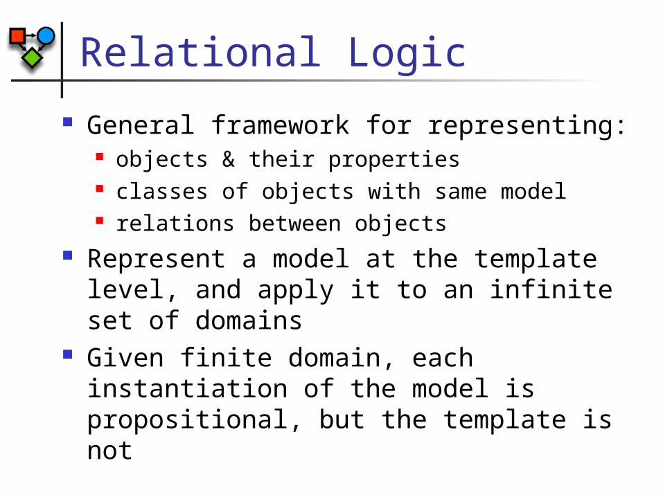
General framework for representing: objects & their properties classes of objects with same model relations between objects

Represent a model at the template level, and apply it to an infinite set of domains

Given finite domain, each instantiation of the model is propositional, but the template is not

Relational Schema Specifies types of objects in domain, attributes of

each type of object & types of relations between objects

Student

Intelligence

Registration

Grade

Satisfaction

Course

Difficulty

Professor

Teaching-Ability

ClassesClasses

AttributesAttributes

TeachRelationsRelationsHas

In

St. Nordaf University

Tea

ches

Tea

ches

In-course

In-course

Registered

In-course

Prof. SmithProf. Jones

George

Jane

Welcome to

CS101

Welcome to

Geo101

Teaching-abilityTeaching-ability

Difficulty

Difficulty Registered

RegisteredGrade

Grade

Grade

Satisfac

Satisfac

Satisfac

Intelligence

Intelligence

HighHigh

Hard

Easy

A

C

B

Hate

Hate

Hate

Smart

Weak

HighLow

Easy

Easy

A

B

C

Like

Hate

Like

Smart

Weak

Relational Logic: Summary Vocabulary:

Classes of objects: Person, Course, Registration, …

Individual objects in a class: George, Jane, …

Attributes of these objects: George.Intelligence, Reg1.Grade

Relationships between these objects Of(Reg1,George), Teaches(CS101,Smith)

A world specifies: A set of objects, each in a class The values of the attributes of all objects The relations that hold between the objects

Binary Relations

Any relation can be converted into an object: R(x1,x2,…,xk)

new “relation” object y, R1(x1,y), R2(x2,y),…, Rk(xk,y)

E.g., registrations are “relation objects”

Can restrict attention to binary relations R(x,y)

Relations & Links

Binary relations can also be viewed as links:

Specify the set of objects related to x via R R(x,y) y x.R1, x y.R2

E.g., Teaches(p,c) p.Courses = {courses c : Teaches(p,c)} c.Instructor = {professors p : Teaches(p,c)}

Relational Bayesian Network

Universals: Probabilistic patterns hold for all objects in class Locality: Represent direct probabilistic dependencies

Links define potential interactions

StudentIntelligence

RegGrade

Satisfaction

CourseDifficulty

ProfessorTeaching-Ability

[K. & Pfeffer; Poole; Ngo & Haddawy]

0% 20% 40% 60% 80% 100%

hard,high

hard,low

easy,high

easy,lowA B C

Prof. SmithProf. Jones

Welcome to

CS101

Welcome to

Geo101

RBN Semantics

Teaching-abilityTeaching-ability

Grade

Grade

Grade

Satisfac

Satisfac

Satisfac

Intelligence

Intelligence

George

Jane

Welcome to

CS101

Difficulty

Difficulty

Welcome to

CS101

low / high

The Web of Influence

0% 50% 100%0% 50% 100%

Welcome to

Geo101 A

C

low high

0% 50% 100%

easy / hard

Why Undirected Models? Symmetric, non-causal interactions

E.g., web: categories of linked pages are correlated

Cannot introduce direct edges because of cycles

Patterns involving multiple entities E.g., web: “triangle” patterns Directed edges not appropriate

“Solution”: Impose arbitrary direction Not clear how to parameterize CPD for variables

involved in multiple interactions Very difficult within a class-based

parameterization[Taskar, Abbeel, K. 2001]

Markov Networks

Laura

Noah

Mary

James

N)(L,N)(M,M)(J,L)(K,L)(J,K)(J,

ZN)M,L,K,P(J,

1

Kyle

0 0.5 1 1.5 2

AAABACBABBBCCACBCC

Template potential

Markov Networks: Review

A Markov network is an undirected graph over some set of variables V

Graph associated with a set of potentials i

Each potential is factor over subset Vi

Variables in Vi must be a (sub)clique in network

i iiZP )(

1)( VV

Relational Markov Networks

Probabilistic patterns hold for groups of objects Groups defined as sets of (typed) elements linked

in particular ways

Study Group

Student2

Reg2GradeIntelligence

Course

RegGrade

Student

Difficulty

Intelligence

0 0.5 1 1.5 2

AAABACBABBBCCACBCC

Template potential

[Taskar, Abbeel, K. 2002]

RMN Language

Define clique templates All tuples {reg R1, reg R2, group G}

s.t. In(G, R1), In(G, R2) Compatibility potential (R1.Grade, R2.Grade)

Ground Markov network contains potential (r1.Grade, r2.Grade) for all appropriate r1, r2

Welcome to

CS101

Ground MN (or Chain Graph)

Welcome to

Geo101

Difficulty

Difficulty

Grade

Grade

Intelligence

Intelligence

George

Jane

Jill

Intelligence

Geo Study Group

CS Study Group

Grade

Grade


Case Study I: Linked Documents

Webpage classification Link prediction Citation matching

Web KB

Tom MitchellProfessor

WebKBProject

Sean SlatteryStudent

Advisor-of

Project-of

Member

[Craven et al.]

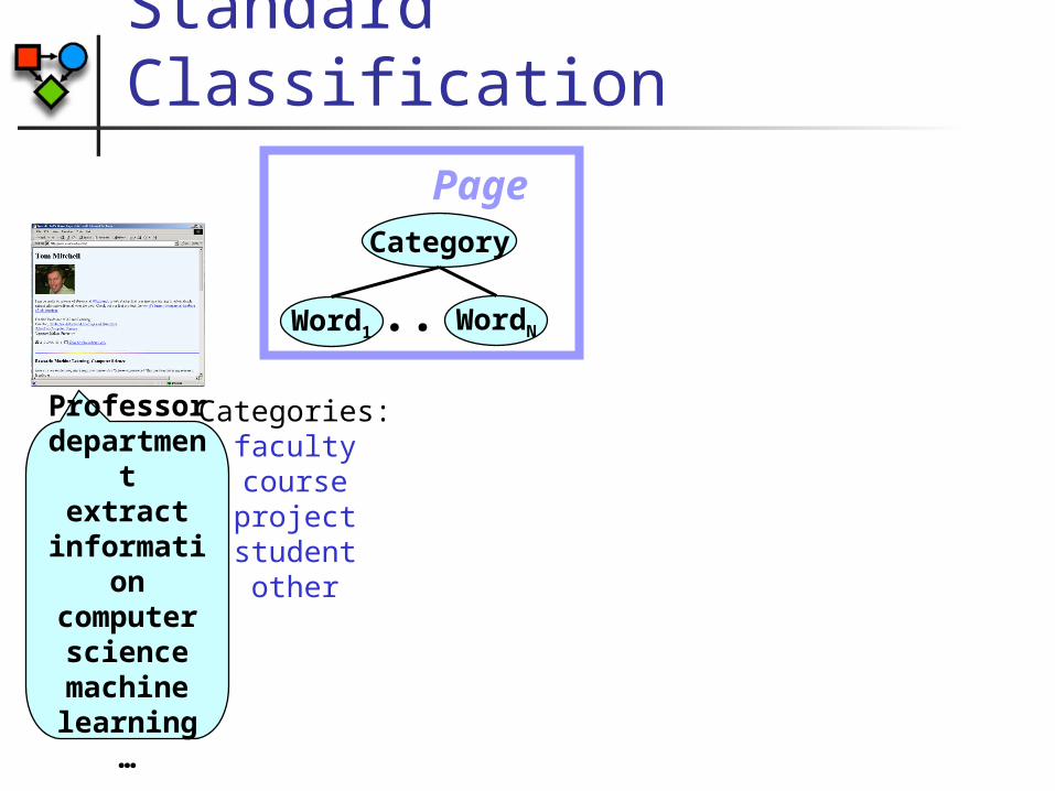
Professordepartment

extractinformationcomputersciencemachinelearning

…

Standard Classification

Categories:facultycourseprojectstudentother

Page

...

Category

Word1 WordN

Standard Classification

...LinkWordN

workingwithTom Mitchell …

Page

...

Category

Word1 WordN

00.020.040.060.080.1

0.120.140.160.18

Logistic

test

set

err

or

4-fold CV:Trained on 3 universities

Tested on 4th

Discriminatively trained naïve Markov

= Logistic Regression

Power of ContextProfessor

?Student? Post-doc?

Model Structure

ProbabilisticRelational

ModelCourse

Student

Reg

Training Data

New Data

Learning

Inference

Conclusions

Collective Classification

Train on one year of student intelligence, course difficulty, and grades Given only grades in following year, predict all students’ intelligence

Example:

[Taskar, Abbeel, K., 2002]

Collective Classification Model

...

PageCategory

Word1 WordN

From-

Link ...

PageCategory

Word1 WordN

To-

Logistic Links

test

set

err

or

00.020.040.060.080.1

0.120.140.160.18

CCCFCPCSFCFFFPFSPCPFPPPSSCSFSPSS

Compatibility (From,To)FTClassify all pages collectively,

maximizing the joint label probability

[Taskar, Abbeel, K., 2002]

More Complex Structure

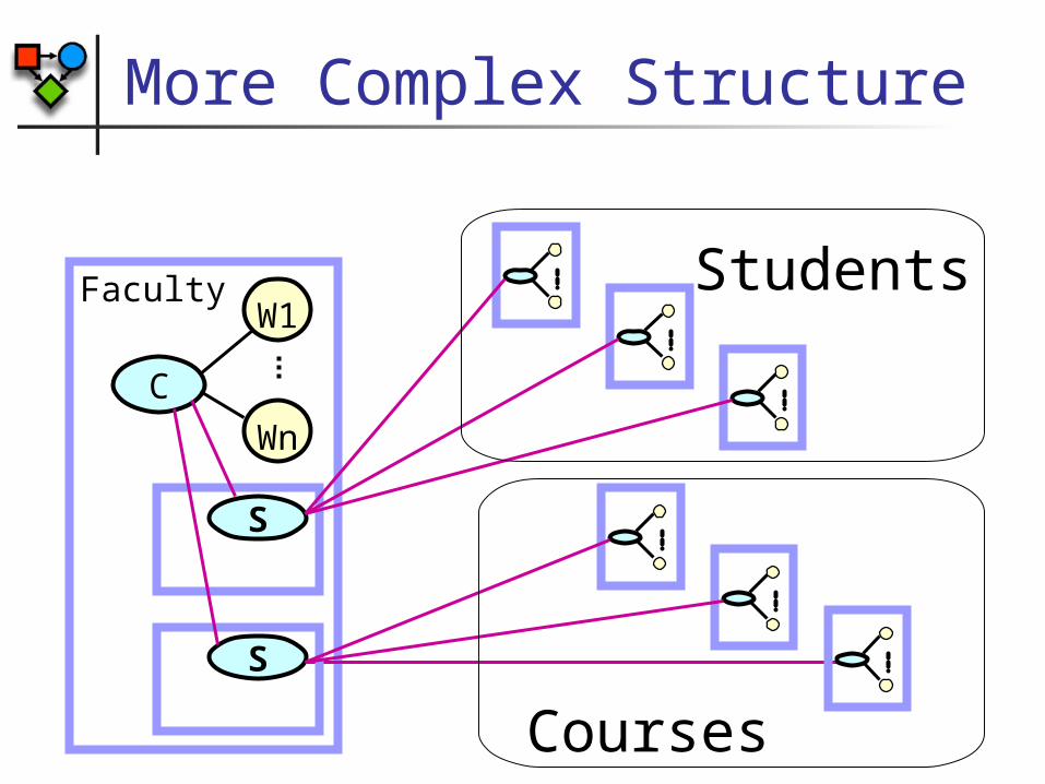
More Complex Structure

C

Wn

W1Faculty

S

Students

S

Courses

Collective Classification: Results

00.020.040.060.080.1

0.120.140.160.18

Logistic Links Section Link+Section[Taskar, Abbeel, K., 2002]

test

set

err

or

35.4% error reduction over logistic

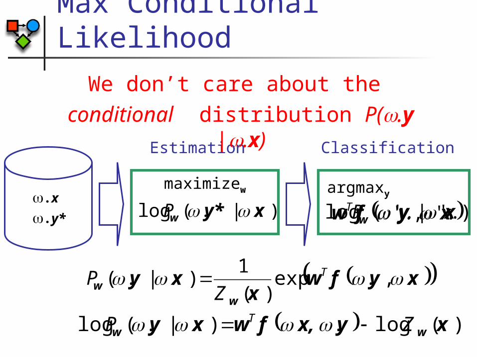
Max Conditional Likelihood

maximizew

Estimation Classification

argmaxy

)(log..).|.(log xyx,fwxy ww ZP T

xyfwx

xyw

w .,.exp)(

1).|.( T

ZP

)'.|'.(log xyw P xyfw '.,'. T).|.(log xy*w P.x

.y*

We don’t care about the conditional distribution P(.y |

.x)

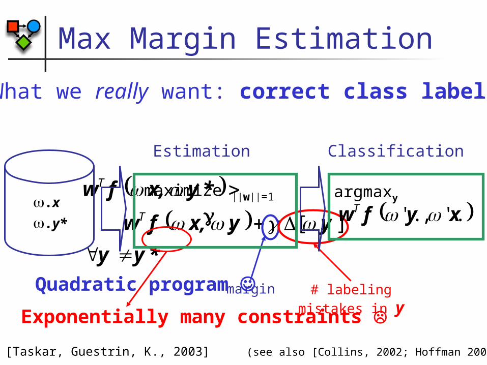
*yy

yyx,fw

*yx,fw

].[..

..

T

T

margin # labelingmistakes in y

Max Margin Estimation

[Taskar, Guestrin, K., 2003] (see also [Collins, 2002; Hoffman 2003])

Quadratic program

Exponentially many constraints

maximize ||w||=1

Estimation Classification

argmaxy xyfw '.,'. T.x

.y*

What we really want: correct class labels

Max Margin Markov Networks

We use structure of Markov network to provide equivalent formulation of QP Exponential only in tree width of network Complexity = max-likelihood classification

Can solve approximately in networks where induced width is too large Analogous to loopy belief propagation

Can use kernel-based features! SVMs meet graphical models

[Taskar, Guestrin, K., 2003]

WebKB Revisited

00.020.040.060.080.1

0.120.140.160.180.2

Test

Err

or

Logistic likelihood max margin

16.1% relative reduction in error relative to cond. likelihood RMNs

Predicting Relationships

Even more interesting: relationships between objects

Tom MitchellProfessor

WebKBProject

Sean SlatteryStudent

Advisor-of

Member

Member

Rel

Flat Model

...PageWord1 WordN

From- ...

PageWord1 WordN

To-

Type

...LinkWord1 LinkWordN

NONEadvisor

instructor

TAmemberproject-

of

Introduce exists/type attribute for each potential link Learn discriminative model for this attribute

Collective Classification: Links

Rel

...

Page

Word1 WordN

From-

...

Page

Word1 WordN

To-

Type

...LinkWord1 LinkWordN

Category Category

[Taskar, Wong, Abbeel, K., 2002]

Link Prediction: Results

Error measured over links predicted to be present

Link presence cutoff is at precision/recall break-even point (30% for all models) 0

5

10

15

20

25

30

Flat Links Triad

...

... ...72.9% relative reduction in error relative to strong flat approach

[Taskar, Wong, Abbeel, K., 2002]

Identity Uncertainty Model

Background knowledge is an object universe A set of potential objects

PRM defines distribution over worlds Assignments of values to object attributes Partition of objects into equivalence classes Objects in same class have same attribute

values

[Pasula, Marthi, Milch, Russell, Shpitser, 2002]

Citation Matching Model*

Each citation object associated with paper object Uncertainty over equivalence classes for papers If P1=P2, have same attributes & links

Author Name

Citation

ObsTitle

Text

* Simplified

Author-as-CitedName

PaperTitle

PubType

Appears-inRefers-toWritten-by

Link chain:Appears-in.Refers-to.Written-by

Title, PubType

Authors

Identity Uncertainty

Depending on choice of equivalence classes: Number of objects changes Dependency structure changes

No “nice” corresponding ground BN

Algorithm: Each partition hypothesis defines simple BN Use MCMC over equivalence class partition Exact inference over resulting BN defines

acceptance probability for Markov chain[Pasula, Marthi, Milch, Russell, Shpitser, 2002]

Identity Uncertainty Results

70

75

80

85

90

95

100

Face RL Reasoning Constraint Average

Phrase Match PRM+MCMC

Accuracy of citation recovery: % of actual citation clusters recovered perfectly

[Pasula, Marthi, Milch, Russell, Shpitser, 2002]

61.5% relative reduction in error relative to state of the art


Case Study II: 3D Objects

Object registration Part finding Shape modeling Scene segmentation

3D Scene Understanding

Goal: Understand 3D data in terms of objects and relations

“puppet holding stick”

3D Object ModelsPose

vari

ati

on

Shape variation

Object models: Discover object parts Model pose variation in terms of parts

Class models: Model shape variation within class

Models learned from data

The Dataset

Cyberware Scans 4 views, ~125k polygons ~65k points each missing surfaces

70 scans

48 scans

Standard Modeling Pipeline

[Allen, Curless, Popovic 2002]

1. Articulated Template 2. Fit Template to Scans

3. Interpolation

A lot of human intervention

Pose or body shape deformations modeled, but not both

Similar to: [Lewis et al. ‘00] [Sloan et al. ’01] [Mohr, Gleicher ’03], …

Data Preprocessing: Registration

Task: Establish correspondences between two surfaces

[Anguelov et al., 2004]

Generative Model

Model mesh X Transformed mesh X’

Deformation / Transformati

on

Goal: Given model mesh X and data mesh Z, recover transformation and correspondences C

Data mesh Z

Data Generation /

Correspondences

C

ix'

Correspondence ck specifies which point x’i generated point zk

ix

kz

[Anguelov, Srinivasan, K., Thrun, Pang, Davis, 2004]

Standard Method: Nonrigid ICP

XZ

c1

c2

Correspondences for different points computed independently

Poor correspondencesPoor transformations

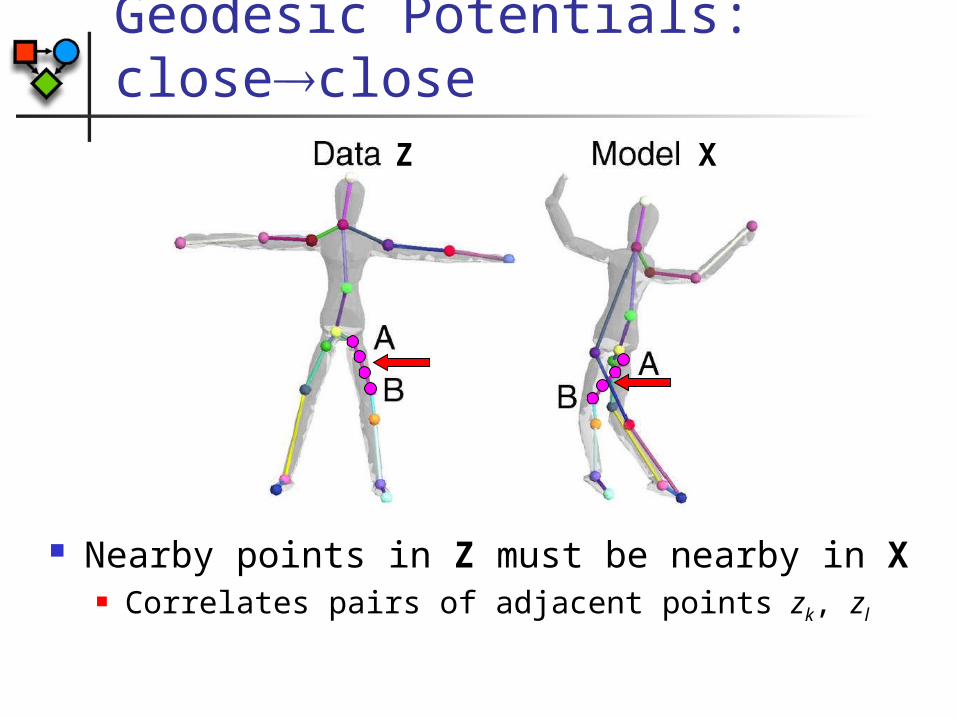
Geodesic Potentials: closeclose

Nearby points in Z must be nearby in X Correlates pairs of adjacent points zk, zl

Z X

Geodesic Potentials: farfar

Distant points in Z must be distant in X Correlates pairs of distant points zk, zl

Z X

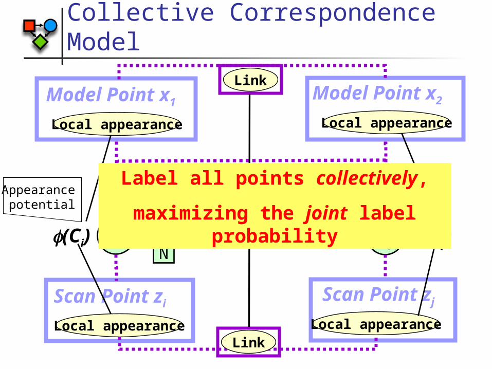
Collective Correspondence Model

Scan Point ziLocal appearance

Model Point x1Local appearance

Scan Point zjLocal appearance

Model Point x2Local appearance

12…N

Link

Link

Ci

(Ci,Cj

)

Deformation potential

Cj(Ci) (Cj)

Appearance potential

Label all points collectively,

maximizing the joint label probability

Inference is hard! Large model, many edges

Exact inference is intractable!

Loopy belief propagation: Approximate inference algorithm Passes messages between nodes in graph Often works fairly well in practice Doesn’t always converge When it does, convergence point not always very

good

Inference is hard! In our case:

With very fine mesh, can converge to poor result Use coarse-grained mesh, and then refine

There are O(n2) “farness” constraints Inference in resulting fully connected model is

completely intractable

Most constraints never relevant Add constraints only as needed

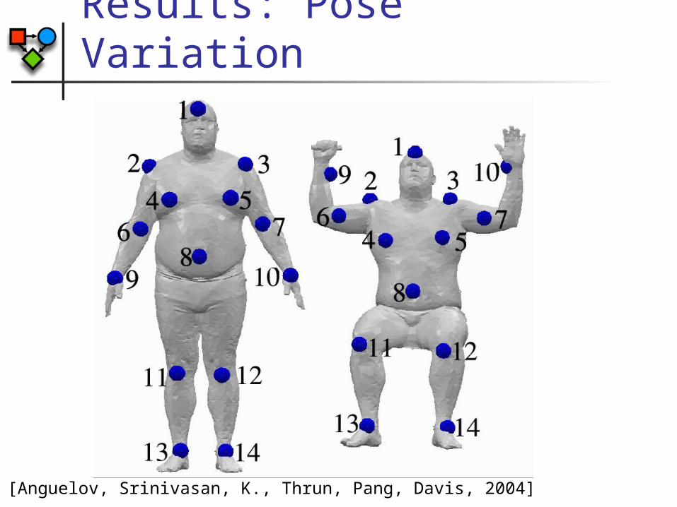
Results: Pose Variation


Results: Shape Variation


Recovering articulated models

Input: models, correspondences

Output: rigid parts, skeleton

[Anguelov, Koller, Pang, Srinivasan, Thrun ‘04]

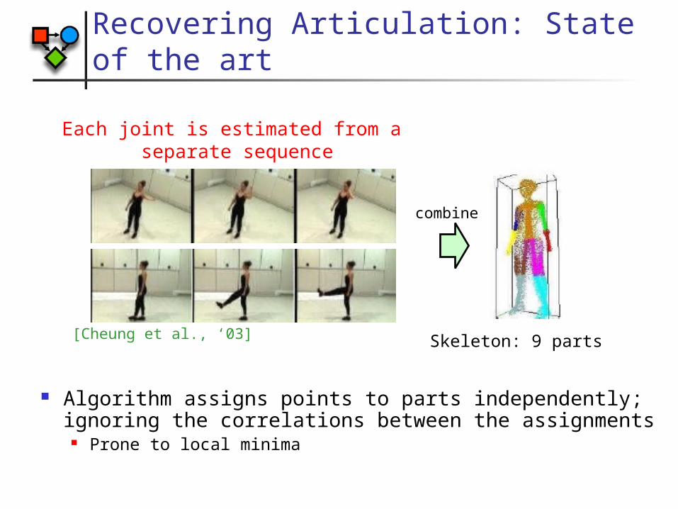
Recovering Articulation: State of the art

Algorithm assigns points to parts independently; ignoring the correlations between the assignments

Prone to local minima

Each joint is estimated from a separate sequence

Skeleton: 9 parts

combine

[Cheung et al., ‘03]

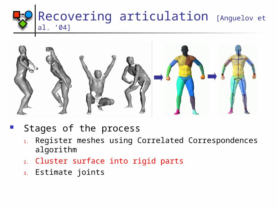
Recovering articulation [Anguelov et al. ’04]

Stages of the process1. Register meshes using Correlated Correspondences

algorithm2. Cluster surface into rigid parts3. Estimate joints

Model Structure

ProbabilisticRelational

ModelCourse

Student

Reg

Unlabeled Relational Data

Learning

Collective Clustering

Given only students’ grades, cluster similar students Given a set of 3D meshes, cluster “related” points

Example:

Clustering of instances

Learning w. Missing Data: EM

Learn joint probabilistic model with hidden vars

EM Algorithm applies essentially unchanged E-step computes expected sufficient statistics,

aggregated over all objects in class M-step uses ML (or MAP) parameter estimation

Key difference: In general, the hidden variables are not

independent Computation of expected sufficient statistics

requires inference over entire network

P(Registration.Grade | Course.Difficulty, Student.Intelligence)

0% 50% 100%

hard,high

hard,low

easy,high

easy,low

Learning w. Missing Data: EM

0% 50% 100%

hard,high

hard,low

easy,high

easy,low

0% 50% 100%

hard,high

hard,low

easy,high

easy,low

0% 50% 100%

hard,high

hard,low

easy,high

easy,low

0% 50% 100%

hard,high

hard,low

easy,high

easy,low

low / higheasy / hard

A B C

CoursesStudents

[Dempster et al. 77]

Collective Clustering Model

Orig pos

PartTransformation

New pos

Model Point

Data Pos

Data Point

Corr

esp

on

dIn

Near

Orig pos

PartTransformation

New pos

Model Point

Data Pos

Data Point

InC

orre

sp

on

d

Associative Markov Nets

yi yj

iji

For K = 2, can be found using min-cut*For K > 2, solve within factor of 2 of optimal

*Greig et al. 89, Kolmogorov & Zabih 02

E.g.: nearby pixels or laser scan points, similar webpagesK

…

1

K K

…

1 2

1 1{1, …,

K}

Finding Parts Hidden variables:

Assignment of points to parts

Parameters: Part transformations

Optimize using EM algorithm

E step performed efficiently using min-cut algorithm

Number of clusters determined automatically

[Anguelov, K., Pang, Srinivasan,Thrun, 2004]

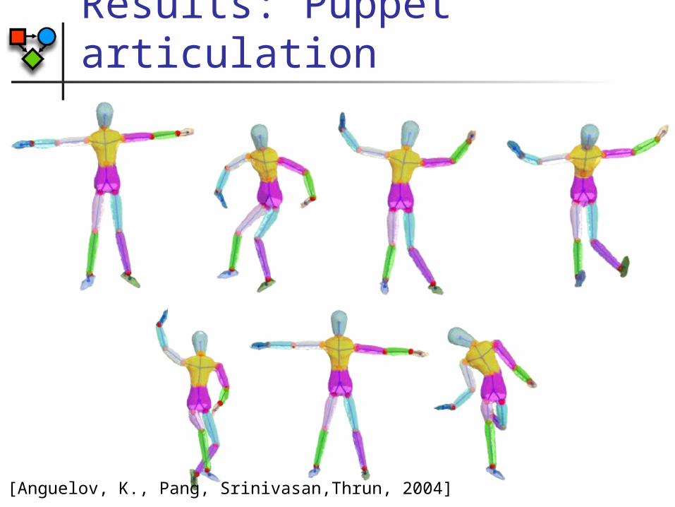
Results: Puppet articulation


Results: Arm articulation


Results: 50 Human ScansTree-shaped skeleton

foundRigid parts found


Modeling Human Deformation

Deformedpolygon

Templatepolygon

Pose deformation

Body shape deformation

Rigid part

rotation

Predict from nearby

Joint angles

Linear subspace(PCA)

[Anguelov, Srinivasan, K., Thrun, Rodgers, Davis, 2005]

Pose Deformationinput

Joint angles Deformations

output

Regression function

Pose deformation


Body Shape Deformationinput

output

Low-dimensional subspace (PCA)

Shape Deformation Model

Shape Transfer


Shape Completion

Sparsesurfacemarkers

Find most probablesurface

w.r.t. model

Joint angles R

Body shape

in PCA space

Completed surface


Partial View Completion


Motion Capture Animation


Segmentation

Train model to assign points to parts Discriminative training using pre-segmented

images

Collective classification Neighboring points more likely assigned to

same part

Use associative Markov network, with min-cut for inference

[Anguelov, Taskar, Chatalbashev, Gupta, K., Heitz, Ng, 2005]

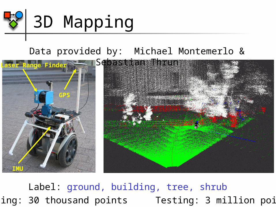
3D Mapping

Laser Range Finder

GPS

IMU

Data provided by: Michael Montemerlo & Sebastian Thrun

Label: ground, building, tree, shrub Training: 30 thousand points Testing: 3 million points

Segmentation results

Hand labeled 180K test pointsModel

Accuracy

SVM 68%

V-SVM

73%

AMN 93%

[Anguelov, Taskar, Chatalbashev, Gupta, K., Heitz, Ng, 2005]

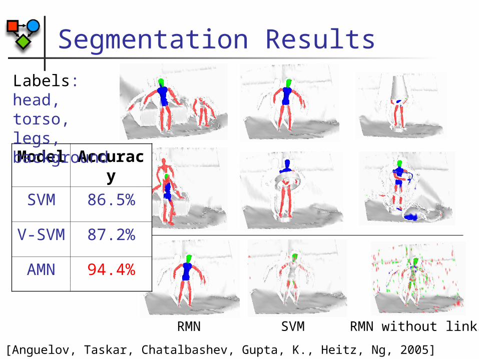
Segmentation Results

Comparison

RMN SVM RMN without links

Model

Accuracy

SVM 86.5%

V-SVM

87.2%

AMN 94.4%

Labels: head, torso, legs, background


Case Study III: Cellular Networks

Discovering regulatory networks from gene expression data Predicting protein-protein interactions

Model Based Approach

Biological processes are about objects & relations

Classes of objects: Genes, experiments, tissues, patients

Properties Observed: gene sequence, experiment

conditions Hidden: gene function

Relations Gene regulation Protein-protein interactions

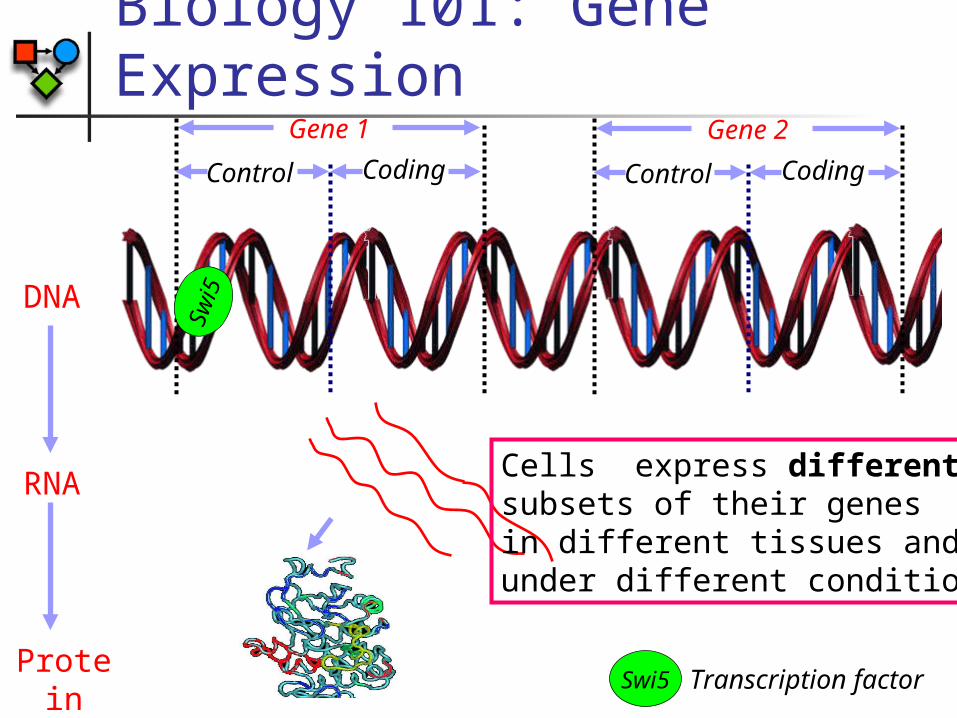
Biology 101: Gene Expression

Gene 2

CodingControl

Gene 1

CodingControl

DNA

RNA

Protein

Swi5 Transcription factor

Sw

i5

Cells express different subsets of their genesin different tissues and under different conditions

Gene Expression Microarrays

Measure mRNA level for all genes in one condition Hundreds of experiments Highly noisy

Expression of gene i in experiment jExperiment

s

Gen

es

Induced

Repressed

Expression level in each module is a

function of expression of regulators

Gene Regulation Model

Experiment

Gene

Expression

Module

Regulator1

Regulator2

Regulator3

Level

Module assignment of

gene “g”

Expression level of Regulator1 in experiment

Segal et al. (Nature Genetics, 2003)

Module Networks

Goal: Discover regulatory modules and their regulators Module genes: set of genes that are similarly controlled Regulation program: expression as function of regulators

Modu

les

HAP4

CMK1 truefalse

truefalse

Global Module Map

Are the module genes functionally coherent?

Are some module genes known targets of the predicted regulators?

Hap4

Xbp1

Yer184c

Yap6

Gat1

Ime4

Lsg1

Msn4

Gac1

Gis1

Ypl230w

Not3

Sip2

12 3 2533414263947 30 4231 36 5 16

Kin82

Cm

k1

Tpk1

Ppt1

8109

Tpk2

Pph3

13 141517

Bm

h1

Gcn20

18 11

46/50

30/50


Wet Lab Experiments Summary

3/3 regulators regulate computationally predicted genes

New yeast biology suggested Ypl230w activates protein-

folding, cell wall and ATP-binding genes

Ppt1 represses phosphate metabolism and rRNA processing

Kin82 activates energy and osmotic stress genes


Human Data Human is a lot more complicated than yeast…

More genes, regulators, noise Less ability to perturb the system

How do we identify “real” regulatory relationships?

Idea: use comparative genomics “Accidental” relationships in expression data

uncorrelated in different species Relevant relationships confer selective

advantage, and are likely maintained

Goal: Discover regulatory modules that are shared across organisms

Gene

Experiment

Expression

Regulator1

Regulator2

Regulator3

Level

Organism 2

Module

Experiment

Gene

Expression

Regulator1

Regulator2

Regulator3

Level

Organism 1

Module

Conserved Gene Regulation Model

Orthologs are more likely to be

in the same module

Regulation programs for the same module

are more likely to share regulators

Goal: Discover regulators that are shared across organisms

Human (90 arrays)Mouse (43 arrays)

Conserved Regulation: Data

Normal brain (4) Medulloblastoma (60) Other brain tumors

(26) Gliomas, AT/RT, PNETs

Normal brain (20) Medulloblastoma

(23)

3718 human-mouse orthologous gene pairs measured in both human & mouse microarrays

604 candidate regulators based on GO annotations Include both transcription factors & signaling proteins

0

500

1000

1500

2000

2500

0 5 10 15 20

Does adding mouse data help?Improvement in Expression Prediction

AccuracyTest Data Log-Likelihood (gain per gene)

Human*

C: bonus for assigning orthologs to corresponding modules

imp

rovem

en

t in

exp

ress

ion

p

red

icti

on

for

un

seen

arr

ays

By combining expression data from two species, we learn a better model of gene

regulation in each

* similar results for mouse

Human-onlymodule network

Conserved Cyclin D Module

34/38 (human), 34/40 (mouse) genes are shared Significant split on medulloblastoma for both human (p < 0.02)

and mouse (p < 10-6), and poor survival in human (p < 0.03)

mouse human

17/22 MB 2/11 MB 23/24 MB 0/19 MB

Cyclin D1 & Medulloblastoma

Cyclin D1 is known to be an important mediator of Shh-induced proliferation and tumorigenesis in medulloblastoma (Oliver, 2003)

mouse human

Conclusion

Under the Hood: Representation

“Correct” modeling granularity is key Too simple miss important structure Too rich cannot be identified from the data

Relational models provide significant value: Exploiting correlations between related

instances Integrating across multiple data sources,

multiple levels of abstraction

Under the Hood: Inference Huge graphical models Exact inference is

intractable 3000-50,000 hidden variables Often very densely connected

Often use belief propagation, but additional ideas key to scaling, convergence:

“Smart” initialization Hierarchical model, coarse to fine Incremental inference, with gradual introduction of

constraints Pruning the space using heuristics

Important to identify & exploit additional structure Use of min-cut for segmentation

Under the Hood: Learning Relational models inherently based on reuse

Fewer parameters to estimate More identifiable

Algorithmic ideas key to good accuracy: Phased learning of model components Discriminative training using max-margin approach

Important to identify & exploit additional structure Convex optimization (relaxed linear programming)

for discriminative training of certain Markov networks

The Web of Influence World contains many different types of

objects, spanning multiple scales Objects are related in complex networks

When we try to pick out anything by itself, we find that When we try to pick out anything by itself, we find that

it is bound fast by a thousand invisible cords that it is bound fast by a thousand invisible cords that

cannot be broken, to everything in the universe.cannot be broken, to everything in the universe.

John Muir, 1869John Muir, 1869

“Web of influence” that provides powerful clues for understanding the world

© daphne koller, 2005 probabilistic models of relational domains daphne koller stanford university

Documents

set of objects

individual objects

propertiesclasses of

differentdata instances

correlateddata instances

shared parameters

heterogeneous instances

regulationsensor data