oautekconf.orgoautekconf.org/wp-content/uploads/2019/09/oautekconf...biennial international...
TRANSCRIPT


FACULTY OF TECHNOLOGY CONFERENCE 2019
(OAUTEKCONF 2019)
“Diversification of Developing Economies: Imperatives for Sustainable Environment & Technological Innovations”
PROCEEDINGS
Volume VII
Edited by
A. A. Akindahunsi, R. N. Ikono, I. P. Gambo, S. A. Adio
ISSN: 2705-3024

Proceedings of the OAU Faculty of Technology Conference 2019 ISSN: 2705-3024
ii
FORWARD
It is my pleasure to heartily welcome all our highly esteemed participants to this 2019 edition of the Biennial International Conference and Exhibitions of the Faculty of Technology, Obafemi Awolowo University, Ile-Ife (OAUTeKConF-2019), with the theme; “Diversification of Developing Economies:
Imperatives for Sustainable Environment & Technological Innovations”, holding between the 22nd to 25th September, 2019.
This year’s conference will witness a major paradigm shift in focus and format, as it will feature several sub-themes addressing various aspects of technological innovations, exhibitions, which will be the centrepiece of the Conference. The Roundtable is expected to focus discourse on the critical research components that will enable the achievement of the desired synergy amongst the three-major stakeholder-groups, for sustainable development. We have invited a set of highly esteemed personalities who have played significant roles in promoting development of human capacity building, expertise in education, industry-manufacturing, research and development, entrepreneurship, technology utilization and management, etc., over the years, as panellists. We are therefore certain that our targeted audience of highly esteemed researchers, entrepreneurs, industrialists, manufacturers, technocrats, management-consultants, scientists and engineers, agents, distributors, policy makers and academics, will bring their wealth of experience and knowledge to bear in tackling these issues in order to address the obvious disconnect in the stakeholder-groups’ relationships, at this forum.
In this 2019 edition of OAUTeKConF, almost all the papers to be presented either orally or as poster have been peer reviewed and thoroughly edited before their inclusion in the proceedings. Going by the quality of the papers, which place a high premium on scholarship and relevance to our national development, and the calibre of personalities presenting keynotes, lead and other technical papers, on a wide range of challenging topics, I am persuaded that an extremely rich cross-fertilization of ideas by participants is guaranteed. The large volume of the conference proceedings will therefore serve as a compendium of intellectual property for researchers, industrialists and policy makers in the country and beyond.
I would like to use this opportunity to thank all spirited individuals and corporate organizations who have generously sponsored this year’s conference. It is my earnest prayer that together, we shall move Nigeria to a greater height, very rapidly.
I wish you all, very exciting and resourceful deliberations and journey mercies back to your destinations at the close of the conference.
Last but not the least, my profound gratitude goes to the Chairman and members of the Conference Planning Committee (CPC), which later devolved into the Local Organizing Committee (LOC), for their outstanding commitment and the technical team of editors who all worked assiduously to ensure that the proceedings of the conference are published. Kudos to you all!
Thank you and God bless you all.
Prof. G. A. Aderounmu Dean, Faculty of Technology

Proceedings of the OAU Faculty of Technology Conference 2019
iii
TABLE OF CONTENT
S/N Title of Paper and Author Page
1. A PATHWAY TO SUCCESSFUL COMMERCIALISATION OF ACADEMIC RESEARCH IN NIGERIA 1
I. O. ABEREIJO AND J. F. OBISANYA
2. A STUDY ON THE EFFECTS OF POULTRY FEATHERS ADDITIVE ON RICE HUSK BRIQUETTES 11
AREMU AKINTOLA MOSES, ADETAN DARE ADERIBIGBE AND OGUNNIGBO CHARLES OLAWALE
3. AN ASSESSMENT OF THE FACTORS INFLUENCING THE ADOPTION OF EDUCATIONAL MANAGEMENT INFORMATION SYSTEM IN SELECTED UNIVERSITIES IN SOUTHWESTERN NIGERIA 18
T.O. AKINWOLE, T.O. OYEBISI AND O.S. AYANLADE
4. AN IMPROVED NETWORK CONGESTION AVOIDANCE MODEL 24
B. O. AKINYEMI AND T. A. ADIATU
5. DESIGN AND CONSTRUCTION OF AN INEXPENSIVE SALT FOG CHAMBER FOR CORROSION TESTING 32
K. NOSA-UGOBOR, O. J. SAHEEB, A. A. DANIYAN, J. O. OLAWALE, O. O. OLORUNNIWO, D. A. ISADARE, F. I. ALO, AND L. E. UMORU.
6. DESIGN AND IMPLEMENTATION OF A NONLINEAR MODEL PREDICTIVE CONTROLLER ON A NON-MINIMUM PHASE QUADRUPLE TANK SYSTEM 39
A.S. OSUNLEKE, A. BAMIMORE, I. A. OYEHAN, O. O. AJANI AND O.A. OLABIYI
7. DESIGN AND IMPLEMENTATION OF GSM-BASED ENERGY THEFT DETECTION IN A SINGLE-PHASE SMART METER 46
D. T. SAWYER AND F. K. ARIYO
8. DEVELOPMENT OF A LOW-COST PROGRAMMABLE DEVICE FOR CONSUMER-END ENERGY MANAGEMENT 52
O. M. ADEMODI, T. P. ADEIFE AND O.P. AWE
9. DEVELOPMENT OF A MINI DUAL-FIRED HEAT TREATMENT FURNACE FOR LOW INCOME COUNTRIES 57
AJIDE O. OLUSEGUN, IDUSUYI NOSA, AJAYI O. KAYODE. ADETUBERU J. ADEOLUWA, ADISA O. AHMED, ISIDORE C. CHUKWUEMEKA
10. DEVELOPMENT OF AN ELECTRONIC LOAD CONTROLLER FOR AN ISOLATED INDUCTION GENERATOR 64
T. U. BADRUDEEN AND O. A. KOMOLAFE
11. DEVELOPMENT OF HOUSEHOLD WATER FILTER FOR WELL WATER TREATMENT IN NIGERIA 70
J.O. JEJE, O.R. ALO AND J.O. ADEFAYE
12. DISTRIBUTION SYSTEM VOLTAGE PROFILE IMPROVEMENT BASED ON NETWORK STRUCTURAL CHARACTERISTICS 75
S. O. AYANLADE AND O. A. KOMOLAFE
Proceedings of the OAU Faculty of Technology Conference 2019
iv
13. EFFECT OF CNTS ON THE TRIBOLOGY AND THERMAL BEHAVIOURS OF AL NANOPOWDER FABRICATED WITH SPS FOR INDUSTRIAL APPLICATION 81
CHIKA OLIVER UJAH, PATRICIA POPOOLA, OLAWALE POPOOLA AND EMMANUEL AJENIFUJA
14. EFFECTS OF CURING METHODS ON COMPRESSIVE STRENGTH OF NORMAL AND RICE HUSH ASH BLENDED CONCRETES 87
C.M. IKUMAPAYI
15. ESTIMATION OF SHEAR STRENGTH PARAMETERS OF BANDED GNEISS DERIVED SOIL USING SELECTED INDEX PROPERTIES 93
G. O. ADUNOYE, O. A. AGBEDE AND M. O. OLORUNFEMI
16. LOAD-DEFORMATION OF KENAF (HIBISCUS CANNABINUS) STEM AT DIFFERENT MATURITY STAGES 98
O. B. FALANA; A. O. ADEBOBOYE; I. O. ADANIKE1, T. M. OLAGUNJU
17. MAPPING OF CARBON NANOTUBE DISPERSION IN BALL MILLED CNT-AL MIXED POWDERS 103
U. ABDULLAH, M. A. MALEQUE, M.Y. ALI AND I. I. YAACOB
18. MODEL IDENTIFICATION OF BIOMASS BOILER SYSTEM USING PRINCIPAL COMPONENT REGRESSION 109
T. A. MORAKINYO AND C. T. AKANBI
19. THE INFLUENCE OF QUENCHING MEDIA ON HARDNESS AND TENSILE PROPERTIES OF AGE-HARDENED 7075 ALUMINIUM ALLOY 119
A. T. ABDULAZEEZ, D. M. AKINWUMI, D. A. ISADARE, K. J. AKINLUWADE, A. A. DANIYAN, T. O. TAIWO, F. I. ALO, A. R. ADETUNJI, AND M. O. ADEOYE
20. A COMPARATIVE STUDY ON THE PHYSICAL PROPERTIES OF BRIQUETTES PRODUCED FROM CARBONIZED AND UNCARBONIZED CORNCOB MATERIAL 127
T. F. OYEWUSI, E. F. ARANSIOLA, T. E. OLALEYE, J. A. OSUNBITAN AND L. A. O. OGUNJIM
21. A PRELIMINARY STUDY OF MASS TRANSIT SYSTEM FOR OBAFEMI AWOLOWO UNIVERSITY - OBAFEMI AWOLOWO UNIVERSITY TEACHING HOSPITAL COMPLEX, ILE-IFE, LINK ROAD 136
H.MOHAMMED, O.K. AKODU AND S. ALALADE.
22. ASSESSMENT OF WATER QUALITY INDEX OF GROUNDWATER RESOURCES IN IWO LOCAL GOVERNMENT AREA, OSUN STATE, NIGERIA 143
Y. O. ADETONA AND K. T. OLADEPO
23. CHEMICAL AND SENSORY PROPERTIES OF PROBIOTICATED DRINKS FROM BLENDS OF AFRICAN YAM BEAN (AYB), SOYBEAN AND COCONUT MILK ANALOGUES 151
A. V. IKUJENLOLA, E. A. ADUROTOYE AND H. A. ADENIRAN
24. DEGRADATION OF ASCORBIC ACID IN ORANGE JUICE FORTIFIED WITH LOW MOLECULAR WEIGHT PEPTIDES OBTAINED FROM PEPSIN HYDROLYZED AMARANTH LEAF PROTEIN 160
A. A. FAMUWAGUN, S. O. GBADAMOSI, K. A TAIWO, R.E. ALUKO, D. J. OYEDELE AND O. C. ADEBOOYE
25. DESIGN MODIFICATIONS AND PERFORMANCE EVALUATION OF A CENTRIFUGAL IMPACT PALM NUTS CRACKER 167
T. A. MORAKINYO
Proceedings of the OAU Faculty of Technology Conference 2019
v
26. DEVELOPMENT AND PERFORMANCE EVALUATION OF AN AUTOMATED CHLORINATION SYSTEM IN WATER TREATMENT PLANT 181
I. A, OKE, D. A. DARAMOLA , J. B., ELUSADE, T.A, ALADESANMI AND S. LUKMAN
27. DEVELOPMENT OF A LABORATORY ROTARY SHAFT TORQUEMETER 189
AJAYI O. K. AND GHAZAL T. O.
28. EFFECTS OF VACUUM DEGASSING ON THE SPLIT MOULD AND COUNTER-GRAVITY PRECISION CASTING OF MINIATURE FIGURINES. 195
G.F. ABASS, T.E. OLAWUYI, B. AREMO, C.T. OKUWA AND K.K. EJEGBU
29. ENGINEERING ECONOMY STUDIES ON DEVELOPMENT AND PRODUCTION OF SPORTS DRINK FROM INDIGENOUS FRUITS 202
A. B. ILORI, B. O. OYEDOYIN, O. B. OLUWOLE, T. E. AKINWALE AND O. V. OKE
30. EVALUATION OF CEMENT KILN DUST-PERIWINKLE SHELL ASH BLEND ON THE COMPACTION BEHAVIOUR OF LATERITIC SOILS FOR SUSTAINABLE HIGHWAY CONSTRUCTION 207
D.U. EKPO, A.B. FAJOBI AND A.L. AYODELE
31. EVALUATION OF SASOBIT POLYMER AS AN ADDITIVE IN BITUMEN AND ASPHALTIC CONCRETE 214
H. MOHAMMED AND S.A. ADEFESOBI
32. FULFILLING BIOMASS DRYING REQUIREMENT FOR SUSTAINABLE DEVELOPMENT OF BIOENERGY: A COMPARATIVE STUDY OF OPEN SUN, SOLAR AND HOT AIR DRYING OF ORANGE WASTE 218
O. O. AGBEDE, A. O. ADEBIYI, E.O. OKE, K. A. BABATUNDE, F.N. OSUOLALE, O.O. OGUNLEYE, S. E. AGARRY AND A.O. ARINKOOLA
33. FUNCTIONAL AND PHYSICO-CHEMICAL PROPERTIES OF MALTED AMARANTH AND ROASTED SESAME FLOUR BLENDS: POTENTIAL BREAKFAST MEAL BASE 226
A.V. IKUJENLOLA, F.O. OJEDOKUN AND S.H. ABIOSE
34. INFLUENCE OF WATER-CEMENT RATIO AND WATER REDUCING ADMIXTURES ON THE REBOUND NUMBER OF HARDENED CONCRETE 234
K. A. OLONADE, O. J. OYEBO AND Y. O. SULAIMAN
35. MECHANISM AND MODELS FOR CHLORIDE REMOVAL FROM WASTEWATERS 243
I.A. OKE, T. A. ALADESANMI, S. LUKMAN, J. S. AMOKO, O. ADEKUNMBI, S. O. OJO, H.O. OLOYEDE , M. D. IDI AND O.T. OYEWOLE
36. MODEL IDENTIFICATION OF BIOMASS BOILER SYSTEM USING PRINCIPAL COMPONENT REGRESSION 251
T. A. MORAKINYO AND C. T. AKANBI
37. OPERATIONAL EVALUATION OF OBAFEMI AWOLOWO UNIVERSITY MAIN GATE – EDE ROAD INTERSECTION 261
H.MOHAMMED, I. A. OYEBODE AND B.D. OYEFESO.
Proceedings of the OAU Faculty of Technology Conference 2019
vi
38. OPTIMIZATION OF BIODIESEL PRODUCTION FROM KHAYA SENEGALENSIS OIL USING HETEROGENEOUS CATALYST 266
E. E. ONOJOWHO, S. O. OBAYOPO AND A. A. ASERE
39. PROSPECTS OF COMBINED PEROXIDE OXIDATION AND AERATION TREATMENT PROCESSES IN ABATEMENT OF POLLUTION CHARACTERISTICS IN CASSAVA PROCESSING WASTEWATER 274
O. A. OMOTOSHO, J. A. OSUNBITAN AND G. A. OGUNWANDE
40. RAPID, ACCURATE AND EFFICIENT SIMULATION AND ANALYSIS OF COMPLEX SYSTEMS USING IMN APPROXIMANTS. 279
O. TAIWO AND T. OLADIPO
41. SYNTHESIS AND MICROSTRUCTURAL ANALYSIS OF FUNCTIONALLY GRADED CU-TI-NI AND ALN COMPOSITE FOR ELECTRICAL APPLICATIONS 283
A. O. OYATOGUN, A. P. I. POPOOLA, O. M. POPOOLA, , E. A AJENIFUJA, F. O. ARAMIDE, G. M. 1OYATOGUN
42. TREATABILITY STUDIES ON RAW WATER FROM APONMU RESERVIOR IN ILARA – MOKIN, , NIGERIA 290
I.A. OKE; D.A. DARAMOLA, A.A. ADENIJI, E.O. FAKOREDE, A. ADANIKIN, K.O. OLABODE, A.ALADEYELU, O.K. AROWOLO, O.V. AGADA, A. AGBOOLA, AND O. GABRIEL
43. A STUDY ON ENERGY EFFICIENCY OF A MANUFACTURING COMPANY 300
A. O. OKE* AND A. O. OYEYEMI
44. PERFORMANCE COMPARISON OF THREAT CLASSIFICATION MODELS FOR CYBER-SITUATION AWARENESS 305
S. S. OLOFINTUYI T. O. OMOTEHINWA, O. H. ODUKOYA AND E. A. OLAJUBU
45. SOLAR ACTIVITY EFFECT ON GPS-DERIVED IONOSPHERIC TOTAL ELECTRON CONTENT VARIATION AT LOW-LATITUDE STATIONS 310
L. G. OLATUNBOSUN, A. O. OLABODE, T. P. OWOLABI AND E. A. ARIYIBI
46. THE SUCTION CONTROL CHARACTERISTICS OF FLOW SEPARATION ON NACA 23012 320
M. O. JULIUS, S. A. ADIO, A. O. MURITALA AND O. I. ALONGE
47. BIOELECTRICITY PRODUCTION AND TREATMENT OF CATTLE ABATTOIR WASTEWATER USING LOCALLY FABRICATED MICROBIAL FUEL CELLS 330
M.O. OYEKANMI AND K. T. OLADEPO
48. NUMERICAL AND EXPERIMENTAL STUDY ON COMBUSTION OF SANDBOX SEED BIODIESEL 339
S. B. AKINTUNDE AND S. O. OBAYOPO
49. DESIGN AND IMPLEMENTATION OF ENHANCED VEHICLE ANTI-THEFT SYSTEM 347
F. O. ASAHIAH AND O. E. ODUJOBI
50. NUMERICAL AND EXPERIMENTAL INVESTIGATIONS INTO THE EFFECTS OF COMPLEX GEOMETRY ON THE MECHANICAL PERFORMANCE OF ALUMINUM 6063 ALLOY. 352
B.O. MALOMO, W.A. TIJANI, A.A. ADEWOLE, T.A. ALO, H.A OWOLABI AND S.A. ADIO

Proceedings of the OAU Faculty of Technology Conference 2019
vii
51. UTILISATION OF PHOSPHORIC ACID TO IMPROVE THE PROPERTIES OF ADOBE BRICKS FOR LOW-COST HOUSING 361
A. O. MOHAMMED, A. L. AYODELE, A. B. FAJOBI, A. A. AKINDAHUNSI AND A. M. OLAJUMOKE.
52. DEVELOPMENT OF SUGENO FUZZY CONTROLLED TRAFFIC SYSTEM FOR Y-ROAD INTERSECTION – UNIVERSITY OF IBADAN CASE STUDY 368
O.E. ADETOYI
53. RE-THINKING ENGINEERING EDUCATION FOR SUSTAINABLE HUMAN DEVELOPMENT ERROR! BOOKMARK NOT DEFINED.
O. A. ODEJOBI
Proceedings of the OAU Faculty of Technology Conference 2019
1
A PATHWAY TO SUCCESSFUL COMMERCIALISATION OF ACADEMIC RESEARCH IN NIGERIA
I. O. ABEREIJO1 and J. F. OBISANYA2 1Institute for Entrepreneurship and Development Studies,
Obafemi Awolowo University, Ile Ife, Nigeria 2Institute for Entrepreneurship and Development Studies,
Obafemi Awolowo University, Ile Ife, Nigeria
[email protected], [email protected]
ABSTRACT Commercialisation of academic research outputs is well known across the globe to be one of the major drivers of economic growth in today’s economic order. Nevertheless, one critical challenge facing academic researchers in developing countries, like Nigeria, is how to successfully cross the ‘valley of death’ between research resources and commercialisation resources. While there are many factors that might be responsible for this, it has been shown, both theoretically and empirically in the extant literature, that quite a number of academic researchers have little or no entrepreneurial knowledge, which is the main missing link. That is, the required set of skills, aptitudes, insights and circumstances necessary to make the connection between academic research and commercial opportunities are still missing. Therefore, this paper is a modest contribution to conceptual discussions on academic entrepreneurship with the view of suggesting an integrated framework that can be used to develop an entrepreneurial behaviour, which is necessary for commercialisation of research outputs. In order to achieve this, a systematic literature review of theoretical and empirical studies is carried out to identify factors which facilitate boundary crossing and support need-driven research. The proposed framework establishes the importance of collaborative research, as well as the need for design research and design thinking to get empathy of the potential users of the research output. Keywords: Academic research, Commercialisation, Academic entrepreneurship, Entrepreneurial behaviours, Entrepreneurship education INTRODUCTION Academic research is one of the indispensable catalysts for advancement of knowledge in the world today and emanates typically from higher education institutions (HEIs) such as university, polytechnic and college of education (Noor, Ismail & Arif, 2014). Răulea, Oprean & Ţîţu (2016) stated that the purpose and function of university have always been knowledge and wealth creation for the benefit of the public. That is, economic development process has been a major role of university in the society. It is on this premise that this paper examined academic research. Furthermore, as noted by Ghilic-Micu, Mircea & Stoica (2011), academic research is a key component often used to rate academic quality of universities in a country, continent and the world at large. Apart from its role in projecting the image of an institution towards funding opportunities, sound academic research also serves as a leverage that builds the capacity of academics and their research students towards the use of all kind of state-of-the-art approaches that meet the needs of the twenty-first century research endeavours around the globe. Over the years, academic research has yielded useful outputs (solutions) that could be categorised as tangible (physical products) and intangible (service) research outputs. These research outputs often lead to all sorts of
innovation which might be incremental, disruptive or radical ones. Commercialisation of these research outputs is necessary to achieving and sustaining economic growth and development of any nation. This is evident in several studies reported in the extant literature (Mulu, 2017). Consequent on the above, majority of the countries in the world are putting in place policies to increase the entrepreneurial activities of their universities and research institutes and also supporting the commercial uptake of technologies generated from these institutions. The policies include promotion of entrepreneurship education and provision of start-up support. The education is targeted at developing motivation and attitudes for self-employment as well as building the skills and competences needed to successfully start-up and grow a business (Hofer & Potter, 2010). Specifically in Nigeria there are policy instruments for facilitating the nation’s transition from a production-based economy to an innovation-based one. One of these instruments is the establishment of the National Office of Technology Acquisition and Promotion (NOTAP) within the Federal Ministry of Science and Technology, and subsequent establishment of Intellectual Property and Technology Transfer Offices (IPTTOs) in some universities, polytechnics and research institutes. As at August 2018, forty-three (43) IPTTOs have been established to
Proceedings of the OAU Faculty of Technology Conference 2019
2
promote interaction and strengthen the linkage between research institutions and industries (NOTAP, 2019). Others are inclusion of entrepreneurship courses and establishment of entrepreneurship development centre (EDC) in all tertiary institutions. Over the years, these efforts have yielded some results, as several empirical studies like Oyewale, 2005; 2006; 2010; Oyewale, Siyanbola, Dada & Sanni, 2007; Adelowo, 2016, as reviewed by Oyewale, Adelowo & Ekperiware (2018), indicate that Nigerian universities and research institutes have developed patentable and commercialisable inventions. Many of these research outputs have also been published by Nigeria Federal Ministry of Science and Technology (see FMST, 2004). In spite of the success stories above, patenting and commercialisation of these research outputs is still very low. In relation to patenting, between 1998 and 2007 out of 4,823 patents filed in Nigeria, only 566 (11.73%) were filed by Nigerian-based applicants while the remaining applications were filed by large companies from advanced countries (Nigerian Law Intellectual Property Watch Inc, 2018). The most recent data published by World Intellectual Property Organisation (WIPO) and The World Bank also show that between 2011 and 2013 there were 156 applications (6%) from Nigerians out of 2,489 applications filed and 123 (7%) of the applications filed by Nigerians were granted out of 1,776 applications granted within the same period (WIPO, 2018; The World Bank, 2018; see also Oyewale, et al., 2018). It is also reported that majority of the research outputs only end up on the shelves of the researchers especially once they are published through academic outlets. Various reasons, such as inadequate infrastructures, poor linkage among the elements of national innovation system, inconsistent enabling policies, finance and so on, are reported to be responsible. It is equally important to note that effort of government is based on the assumption that academic researchers have entrepreneurship mindset. As noted by Ventakataraman (1997), the ability to make the connection between specific knowledge and a commercial opportunity requires a set of skills, aptitudes, insights and circumstances that are neither uniformly nor widely distributed. Therefore, the cultural difference between academia and the marketplace and the inability of researchers to make the connection between knowledge and business opportunities might explain the reason for the existence of the valley of death between the research laboratory and the marketplace, especially in Nigeria (Abereijo, 2015). From the available literature on commercialisation of research outputs from Nigeria tertiary institutions, authors have focused on institutional networking among the elements of national innovation system (Siyanbola, Olamade, Yusuff & Kazeem, 2012; Oyedoyin, Ilori, Oyebisi, Oluwale & Jegede, 2013; Ogunwusi & Ibrahim, 2014; Oyewale, et al., 2018), factors hindering commercialisation and policy requirements (Egbetokun, Siyanbola & Oyewale, 2011; Siyanbola, et al., 2012;
Yusuf, 2012) and importance of entrepreneurship culturing of these institutions (Ugonna & Onwualu, 2016; Onwualu, 2012). But none has come up with a framework that shows the connection between entrepreneurship process and multi-disciplinary researches with commercialisation of research outputs. Therefore, the main purpose of this paper is to suggest a framework that shows the connection between the processes involved in research and entrepreneurship which can lead to commercialisation. THEORETICAL BACKGROUND The relevant theoretical foundation for the proposed framework in this paper is based on the concept of research, entrepreneurial and market orientation as well as communities of practice. Each of these concepts is explained below. Concept of Research Research, as it relates to university, is targeted at generating new knowledge and or advancing the existing one. Traditionally therefore, researchers in university have a strong interest in pursuing novel ideas so as to discover new information (knowledge) in their field rather than conducting researches that are problem-driven or for developing a commercialisable product or service (Kwok, n.d.). Equally important to researchers is educational impact of their research results. Hence, the results are usually published in peer review academic journals and or books as well as presented at academic conferences. It is believed that the publications and presentations will not only inspire other scholars in that discipline, the channels also open up avenue for more researches for other researchers within and outside the discipline. In addition, as teachers, the research findings also enrich their teaching which further contribute to human development. In recent years however, government and public are showing more interest in the practicality of researches from ivory tower. This is because a substantial number of researches are funded by government, industry and philanthropic agencies. Therefore, universities are expected, not to limit their research activities to the production of new knowledge (research), but also to engage with societal needs and market demands by linking the activities with their socio-economic context (Pinto, Cruz & de Almeida, 2016). Hence, commercialisation of research findings is expected to be a key component of the research mission such that novel ideas, techniques and products can enter the marketplace for the benefit of different stakeholders (Vanderford & Marcinkowski, 2015). This is referred to the third mission of university, defined as the social, enterprise and innovative activities that universities perform in addition to teaching and research tasks (Zomer & Benneworth, 2011). The growing importance of third mission activities aimed at commercialising research findings and creating more entrepreneurial academics has now broadened the scope of research activities. That is, academic researchers are
Proceedings of the OAU Faculty of Technology Conference 2019
3
also expected to focus on research and experimental development, which based on Frascati Manual, is activities comprise creative work undertaken on a systematic basis in order to increase the stock of knowledge, including knowledge of man, culture and society, and the use of this stock of knowledge to devise new applications (OECD, 2015). Research Commercialisation Though it is widely acknowledged that turning research outputs into useful marketable products or services is a means of maximising the return on public investment in research activities in form of economic, social and environmental benefits; but there is no consensus in the definition of research commercialisation (see Åstebro, 2004; Association of University Technology Managers, 2018). This is as a result of differences in the range of activities encompassed by the term, as well as, the impact of the definition on the measurement and assessment of research commercialisation activities in publicly funded research institutions (Muir, Arthur, Berman, Sedgley, Herlick & Fullgrabe, 2005). The definition put forth in the report to the Coordination Committee on Science and Technology, Australia is adopted in this paper. It is defined as the means by which universities’ and publicly funded research agency’s (PFRA) research generates commercial benefit, thereby contributing to (Australia’s) economic, social and environmental well-being. This is achieved through developing intellectual property, ideas, know-how and research-based skills resulting in new and improved products, services and business processes transferable to the private sector (Muir, et al., 2005). The different ways of commercialising research outputs could be through a university spin-off, licensing or sales of intellectual property or cooperation between researchers and private organisations (Hamano, 2011). While spin-offs are companies founded by university employees and refer to their founders as academic entrepreneurs (Zhang, 2009), licensing is a contractual method of applying intellectual property by transferring rights to other firms while retaining ownership (Byers, Dorf & Nelson, 2011). Entrepreneurial Orientation Entrepreneurial orientation is one of the concepts within entrepreneurship research that describes the pattern of behaviour which makes one firm to be more entrepreneurial than others. The concept, which was reconceptualised by Lumpkin & Dess (1996), is defined as the processes, practices and decision-making activities that lead to the act of entrepreneurship or new entry, that is, the act of launching a new venture (Lumpkin & Dess, 1996). The five dimensions used for characterising the entrepreneurial processes are autonomy, innovativeness, risk-taking, proactiveness and competitive aggressiveness. It manifests within a firm’s managerial philosophies, decision-making practices and its strategic behaviour (Anderson, Covin & Slevin, 2009; Wales, 2016). Though entrepreneurial orientation concept has its origin on strategy and indicates the presence of entrepreneurship within the organisation (Yang, 2008),
yet all the identified pattern of behaviour can be viewed as characteristics of individuals with an entrepreneurial orientation (DuBrin, 2012). The implication of this is that, both at individual and institution levels, an entrepreneurial mindset should be nurtured, through various methods and materials, to enhance the ability of researchers to recognise and analyse entrepreneurial opportunities. Market Orientation Market orientation (MO) which was initially based on the marketing concept was popularised in the 1990s as a result of two research works sponsored by the Marketing Science Institute. The publications (Kohli & Jaworski, 1990; Narver & Slater, 1990) that arose from this study impacted significantly on the studies relating to the problems of marketing then, and also led to the first definition of MO. Kohli & Jaworski (1990) define it as the organisation-wide generation of market intelligence pertaining to current and future customer needs, dissemination of the intelligence across departments and organisation-wide responsiveness to it. Narver & Slater (1990) define MO based on its three components which are customer orientation, competitor orientation and inter-functional coordination, as well as its decision criteria, that is, long-term focus and profitability. While customer orientation and competitor orientation involve efforts of the organisation at understanding the target customers and what its competitors are doing respectively, inter-functional coordination is the organisational culture that orients employees in all departments of a business unit toward understanding the firm’s market in terms of both customers and competitors (Dev, Zhou, Brown & Agarwal, 2009). Putting the two definitions together, the goal of MO is about continual collection of information about target customers’ needs and competitors’ capabilities with the intention of providing customers with value that is superior to other competitors on a sustained basis. This must, however, not limited to the organisation’s marketing department, but ensuring that it becomes organisation-wide culture. That is, the norms and beliefs that shape an integrated organisational strategy for sensing changing customer demand and competitive challenges as well as anticipating future market conditions are enshrined within the organisation (Dev, et al., 2009). Within the context of this paper, MO of academic researcher is important considering the positive impact of MO on business performance. Hence, researchers are expected to be skilful both in the conduct of research and in recognition of the market acceptance of the inventions or research outputs (Kadir, 2017). It is then research output is qualified as been commercially viable. Whether the transition from laboratory to market is by technology-push (supply-orientation) or market-pull (demand-orientation) the critical factor in the successful commercialisation of research findings is the match between research outcome and market needs. That is, there must be problem-solution fit and product-market fit
Proceedings of the OAU Faculty of Technology Conference 2019
4
(Osterwalder, Pigneur, Bernarda & Smith, 2014). Problem-solution fit occurs when the value proposition of the research output perfectly matches the needs and problems of target customer, and product-market fit is achieved when the target customers accept the value proposition and are willing to pay for it. Communities of Practice Recently the importance of communities of practice (CoP) to pursue collaborative innovation activities is receiving attention by academic scholars. This is because the platform can be used to undertake innovative projects for local development. The concept was coined by Etienne Wenger and Jean Lave as an approach to learning that focuses on people and the social relationships and structures that allow them to learn together (Lave & Wenger, 1991; Wenger, 1999). It is defined as groups of people who share a concern or a passion for something they do, and learn how to do it better as they interact regularly (Wenger-Trayner, 2015). As explained by the proponents of this concept, CoP differs from project teams or working group because it is essentially informal, voluntary, self-selecting and self-organising. The communities also have three defining characteristics, which are the domain, the community and the practice. Domain is the common interest that links the community, the community is the joint activities in which members engage, and the practice refers to the shared stories, tools and resources from which the group can draw (Lowitt, Hickey, Ganpat & Phillip, 2015). Moreover, the word ‘community’ indicates that communities of practice are not limited by boundaries imposed by geography, sector or function, but defined by common tasks and work interests. Therefore, since communities of practice are not limited by traditional boundaries it can serve as locus for community of innovation whose interest is to learn and co-produce knowledge for practical application and solutions to current challenges. Communities of practice, like trans-disciplinary approach to research programme, can serve as a platform for solving social and environmental problems by developing knowledge and innovations (product, process or service) that have real-world impact. Empirical Evidences on Key Factors in Commercialising Research Outputs Various studies have been conducted on the issues relating to commercialisation of research results from universities. These include factors influencing commercialisation (Behboudi, Jalili, & Mousakhani, 2011; Nikulainen & Tahvanainen, 2013; Masudian, Farhadpoor, & Ghashgayzadeh, 2013; Jahed & Arasteh, 2014), key success factors of commercialisation (Åstebro, 2004; Baaken & Plewa, 2007; Khademi & Ismail, 2013; Safiah, Norain, Nor & Jailani, 2014), commercialisation barriers (Czemiel-Grzybowska & Brezeziński, 2015; Vanderford, N.L. & Marcinkowski, 2015; Ansari, Armaghan & Ghasemi, 2016), commercialisation processes - activities and stages (Australian Centre for Innovation, 2002; Harman, 2010)
and commercialisation mechanisms (Collier, 2007; Wnuk, Mazurkiewicz & Poteralska, 2016). Within the context of this paper, attention is focused on the factors that are critical for laying the foundation that can lead to successful commercialisation of research outputs, especially during research initiation and execution stages. The outcome of the study conducted by Georgia Research Alliance on the failure modes of 119 start-ups, reported by Lee, Lee, Klm & Choi (2015), showed that 29% failed because of technological failure, 27% due to management dysfunction, while 20% and 10% failed because of market related issues and poor business model respectively. Only small percentages, that is, 4%, 7% and 6% of these start-ups failed because of IP protection problem, illiquidity and relocation respectively. The implication of these data, as noted by Lee et al (2015), is that IP related issues and illiquidity that are considered as the most significant problem, that start-ups face, are not so. In addition, the case study of the story of two successful research outputs (TyhiDot and LTK omega plus) in Malaysia revealed that the needs as well as the design and development criteria of the market place are already evident before the research was carried out (Baharudin, 2016). For example, the markets needs identified for TyhiDot are rapid diagnostic tests which are specific, sensitive, easy to perform, have built-in-controls, cost effective, do not require refrigeration, absence of culture facilities, minimal lab infrastructure, lack of electricity, lack of trained personnel and transportation without cold chain. It was on the basis of these needs that both the research activities and commercialisation processes were implemented. LTK omega plus was developed based on the need for a technology that could assist them with a product that offers meaningful differentiation that meets the healthy eating trend of consumers in the market place. Therefore, the consistent factors, in the empirical literature, for successful commercialisation of research outputs are summarised as need-based approach, lean start-up principles, reality checks, trans-disciplinary approach and appropriate rewarding system. The importance of need-based approach can be seen from the understanding that innovation is a complex, often non-linear process, which requires a lot of iteration between innovation stages. Hence, the process should start with defining a particular user need or market segment so as to provide useful insights into research and product development processes. While there are significant science and technology activities in Nigeria, majority of the outputs from these activities are not market-oriented and thus not readily exploitable for commercial purpose. Learn start-up, which is a principled approach to new product development, provides a scientific approach to creating and managing start-ups so as to get a desired product or service to customers (Ries, 2018). A core component of lean start-up methodology is the build-
Proceedings of the OAU Faculty of Technology Conference 2019
5
measure-learn feedback loop, which starts with figuring out the problem that needs to be solved, then development of a minimum viable product (MVP), as well as measurement and learning based on actionable metrics that can demonstrate cause and effect question (Reis, 2018). According to Steve Blank, one of the pioneers of the lean start-up movement in Silicon Valley, the approach has three distinct characteristics. That is, it favours experimentation over elaborate planning, prioritises customer feedback over intuition and emphasises iterative design over traditional ‘big design up front’ development (Blank, 2013). Reality check is closely related to the lean start-up principle because, as Lee et al (2015) noted, getting timely feedback from potential investors and consumers helps the start-ups avoid the presumption that the technology will work as proposed o a ripe market is somewhere out there waiting for the technology to be commercially available. Reality check, using the lean start-up methodology, will help to establish sustainable market for envisaged research outputs. Also, trans-disciplinary approach to research process is an important factor to successful commercialisation because it forges bridges between disciplines in effort to solve complex problems and situation (McGregor, 2004). Therefore, formation of communities of practice by researchers from various disciplines and industry experts is very important. While the academic researchers will provide the conceptual, theoretical and methodological aspects of the research, the industry experts (who may be successful serial entrepreneurs or senior executives at large companies) provide advice on technology commercialisation and marketing. Lastly, as regards rewarding system, it has generally been noted in various studies that universities do not factor technology transfer and commercialisation into performance reviews, promotions and tenures of their researchers (Yaakub, Hussain, Rahman, Zainol, Mujan I, Jamsari, Sulaiman & Jusoff, 2011; Lee et al., 2015). Hence, an effective incentive design appears to be a key factor to building a successful platform for research outputs commercialisation.
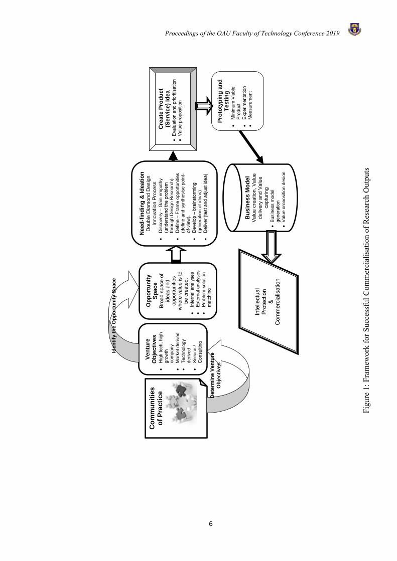
Framework for Successful Commercialisation of Research Outputs While recognising the importance of various components of the innovation ecosystem and larger national innovation system to the commercialisation success of research outputs from universities, the focus of this paper is on laying proper foundation for the commercialisation of research outputs from universities. A review of various models of commercialisation of research results from universities carried out by Lotfollah, Akbar, Abedin & Hossein (2014) revealed that there are different point of views to the model of commercialisation (see Cooper, 1983; Rothwell and Zagveld, 1985; Jolly, 1997; Goldsmith, 2003; Göktepe, 2004; Karlsson, 2004; Mahdi, 2010; University of British Columbia, 2013). The summary of these models is that commercialisation
process starts with idea generation, conducting research on the idea, achieving the desired results, documentation, transfer of results and commercialisation (Lotfollah, et. al., 2014). The proposed framework (figure 1) suggests that the starting point of the pathway to successful commercialisation of academic research outputs is the establishment of communities of practice which include academics from different disciplines and industry experts who will provide advice on technology commercialisation and marketing. The venture objective is thereafter determine as to whether the goal is to develop product that is high tech leading to high growth company, or whether it will be market derived or technology derived, or to provide service or consulting. Next to venture objective determination is identification of opportunity space, which according to Innovation Hub (2019), lies in the intersection of four different subspaces (problem space, solutions space, business space and company space). This is when a many potential venture ideas that are linked to needs, inefficiencies, problems and opportunities are identified (Vlerick Leuven Gent Management School, 2019). Furthermore, need-finding and ideation, which involves watching and asking potential users to learn about their goals and values to be able to uncover user needs and opportunities for improvements is conducted to discover, define, develop and deliver (Javaid, 2014). This ultimately leads to creation of product (service idea), prototyping and testing and generation of business model and value proposition design. The pathway ends with product (service) that can be protected or commercialised
Proceedings of the OAU Faculty of Technology Conference 2019
6
Co
mm
un
itie
s
of
Pra
cti
ce
Ve
ntu
re
Ob
jecti
ve
s
•H
igh
tech
, hig
h gr
owth
co
mpa
ny
•M
arke
t der
ived
•
Tech
nolo
gy
deriv
ed
•Se
rvic
e /
Con
sulti
ng
•D
ete
rmin
e V
en
ture
Ob
jecti
ves
Op
po
rtu
nit
y
Sp
ac
e
Broa
d sp
ace
of
idea
s an
d op
portu
nitie
s w
here
val
ue is
to
be c
reat
ed.
•In
tern
al a
naly
ses
•Ex
tern
al a
naly
ses
•Pr
oble
m-s
olut
ion
mat
chin
g
Ne
ed
-fin
din
g &
Id
eati
on
D
oubl
e D
iam
ond
Des
ign
Inno
vatio
n Pr
oces
s •
Dis
cove
ry –
Gai
n em
path
y (u
nder
stan
d th
e pr
oble
m
thro
ugh
Des
ign
Res
earc
h).
•D
efin
e –
Fram
e op
portu
nitie
s (d
efin
e an
d sy
nthe
sise
poi
nt-
of-v
iew
). •
Dev
elop
– b
rain
stor
min
g (g
ener
atio
n of
idea
s)
•D
eliv
er (t
est a
nd a
djus
t ide
a)
Iden
tify
th
e O
pp
ort
un
ity S
pace
Cre
ate
Pro
du
ct
(Se
rvic
e)
Idea
•Ev
alua
tion
and
prio
ritis
atio
n •
Valu
e pr
opos
ition
Pro
toty
pin
g a
nd
T
esti
ng
•
Min
imum
Via
ble
Prod
uct
•Ex
perim
enta
tion
•M
easu
rem
ent
Bu
sin
es
s M
od
el
Valu
e cr
eatio
n, V
alue
de
liver
y an
d Va
lue
capt
urin
g •
Busi
ness
mod
el
gene
ratio
n •
Valu
e pr
opos
ition
des
ign
Inte
llect
ual
Prot
ectio
n &
Com
mer
cial
isat
ion
Figu
re 1
: Fra
mew
ork
for S
ucce
ssfu
l Com
mer
cial
isat
ion
of R
esea
rch
Out
puts
Proceedings of the OAU Faculty of Technology Conference 2019
7
CONCLUSION
Both theoretical and empirical literatures were reviewed in this paper on the concept of research, entrepreneurial and market orientation as well as communities of practice. The proposed framework suggests seven major points along the pathway for successful commercialisation of research results. The framework being proposed can assist higher education institutions put in place structure and policies that can facilitate the ability of researchers to cross the ‘valley of death’. REFERENCES
Abereijo, I.O. (2015). “Transversing the ‘valley of death’: Understanding the determinants to commercialisation of research outputs in Nigeria”. African Journal of Economic and Management Studies, 6(1), 90-106.
Anderson, B. S., Covin, J. G., & Slevin, D. P. (2009). Understanding the relationship between entrepreneurial orientation and strategic learning capability: an empirical investigation. Strategic Entrepreneurship Journal, 3(3), 218-240.
Ansari, M-T; Armaghan, N.; Ghasemi, J. (2016). “Barriers and solutions to commercialization of research findings in Schools of Agriculture in Iran: A qualitative approach. International Journal of Technology, 7(1), 5-14. Accessed on 2 June, 2018 at http://www.ijtech.eng.ui.ac.id/old/index.php/journal/article/view/1459.
Association of University Technology Managers (2018). “About technology transfer”. Accessed on 26 May 2018 at https://www.autm.net/autm-info/about-tech-transfer/about-technology-transfer/
Åstebro, B.T. (2004). “Key success factors for R&D project commercialisation”. IEEE Transactions on Engineering Management, 51(3), 314-321.
Australian Centre for Innovation (2002). “Best practice processes for university research commercialisation”. Final report submitted to the Department of Communication, Information Technology and the Arts, Australia. Accessed on 2 June 2018 at www.howardpartners.com.au/publications/best-practice-processes.pdf.
Baaken, T. & Plewa, C. (2007). “Key success factors for research institutions in research commercialisation and industry linkages: Outcomes of a German/Australian cooperative project”. In Sherif, M.H. & Khalil, T.M. (Eds.), Management of Technology: New Directions in Technology Management. U.K.: Elservier Ltd
Behboudi, M.; Jalili, N.; & Mousakhani, M. (2011). “Examine the commercialisation research outcomes in Iran: A structural equation model”.
International Journal of Business and Management, 6(7), 261-2715. doi:10.5539/ijbm.v6n7p261.
Blank, S. (2013). “Why the lean start-up changes everything”. Harvard Business Review, May Issue. Accessed on 30 May, 2018 from https://hbr.org/2013/05/why-the-lean-start-up-changes-everything.
Byers, T. H.; Dorf, R.C.; & Nelson, A.J. (2011). Technology Venture from Idea to Enterprise. 3rd ed. Printed in Singapore. The McGraw-Hill Companies.
Collier, A. (2007). “Australian framework for the commercialisation of university scientific research”. Prometheus – Critical Studies in Innovation, 1, 51-68.
Cooper, R.G. (1983). “A process model for industrial new product development”. IEEE Transactions on Engineering Management, 30(1), 2-11.
Czemiel-Grzybowska, W.; & Brezeziński, S. (2015). “Selected barriers management of commercialisation in the international university research”. Polish Journal of Management Studies, 12(2), 59-68.
DEST 2004, Definitions and Methodological Notes—Statistics on Science and Innovation, p. 28.
Dev, C.S.; Zhou, K.Z.; Brown, J. & Agarwal, S. (2009). “Customer orientation or competitor orientation: Which marketing strategy has a higher payoff for hotel brands?”. Cornell Hospitality Quarterly, 50(1), 19-28. Doi:10.1177/1938965508320575
DuBrin, A.J. (2012). Leadership: Research findings, practice and skills (8th edition).
Egbetokun, A.A.; Siyanbola, W.O. & Oyewale, A.A. (2011). “From lab to market: Issues in industry-academy cooperation and commercialisation of R&D outputs in Nigeria”. In Pablos, P.O.; Lee, W.B. & Zhao, J. (Eds.), Regional innovation systems and sustainable development: Emerging technologies. IGI Global: Hershey, New York.
FMST (2004). “Profiles on selected commercialisable research and development results”. Accessed on 26 May 2018 at https://www.cepal.org/iyd/noticias/pais/9/31489/Doc_Nigeria_3.pdf
Ghilic-Micu, B., Mircea, M., & Stoica, M. (2011). Knowledge based economy–technological perspective: implications and solutions for agility improvement and innovation achievement in higher education. Amfiteatru Economic Journal, 13(30), 404-419.
Göktepe, D. (2004). “Investigation of university industry technology transfer cases: A conceptual and methodological approach”. Division of Innovation – LTH.
Proceedings of the OAU Faculty of Technology Conference 2019
8
Goldsmith H.R., Model of Commercialization, Arkansas Small Business and Technology Development Center, Available from: http://asbdc.ualr.edu/technology/commercialization/the model.asp.
Hamano, Y. (2011). “Commercialisation procedures: Licensing, spin-offs and start-ups” World Intellectual Property Organisation working paper.
Harman, G. (2010). “Australian university research commercialisation: Perceptions of technology transfer specialists and science and technology academics”. Journal of Higher Education Policy and Management, 32(1), 69-83.
Hofer, A-R. & Potter, J. (2010). “University entrepreneurship support: Policy issues, good practices and recommendations”. A note prepared in November 2010 for the directing committee of the local economic and employment development programme of the OECD. Accessed on 22 May 2018 at www.oecd.org/edu/imhe/46588578.pdf
Innovation Hub (2019). How are the opportunity spaces defined? Innogy innovation hub at the annual ISPIM conference. Accessed on 20 August, 2019 at https://innovationhub.innogy.com/news-event/177knCFEniSIMmSaG8qEU6/how-are-the-opportunity-spaces-defined--innogy-innovation-hub-at-the-annual-ispim-conference
Jahed, H. & Arasteh, H.R. (2014). “Organisational factors influencing on commercialisation of research results” Quarterly Journal of Innovation and Entrepreneurship, 2(4), 5-22.
Javaid, R. (2014). “What is needfinding?”. Accessed on 20 August, 2019 at https://www.slideshare.net/RizwanJavaid/needfinding-36845052
Jolly, V.K. (1997). Commercialising new technologies: Getting from mind to market. Boston, Mass: Harvard Business School Press.
Kadir, B. (2017). “Market-oriented R&D commercialisation at public universities and government research institutes in Malaysia: Issues and potential research areas”. Journal of Engineering and Applied Sciences, 12(6), 1386-1392.
Karlsson, M. (2004). “Commercialisation of research results in the United States: An overview of federal and academic technology transfer”. ITPS, Swedish Institute for Growth Policy Studies. Accessed on 4 June, 2018 at http://urn.kb.se/resolve?urn=urn:nbn:se:kth:diva-70161.
Khademi, T. & Ismail, K. (2013). “Commercialisation success factors of university research output”. Jurnal Teknologi, 64(3), 137-141.
Kohli, A.K. & Jaworski, B.J. (1990). “Market Orientation: The construct, research propositions, and managerial implications”. Journal of Marketing, 54, pp. 1–18.
Kwok, K. (n.d). “Academic research at university”. Accessed on 26 May, 2018 at https://www.cuhk.edu.hk/clear/rs/academic_research.pdf
Lave, J.; & Wenger, E. (1991). Situated learning. Legitimate peripheral participation. Cambridge, UK: University Press.
Lee, J.; Lee, J.; Klm, B.; & Chol, Y.J. (2015). “Study for main factors of technology commercialisation by its current process analysis”. Indian Journal of Science and Technology, 8(S1), 391-397. DOI: 10.17485/ijst/2015/v8iS1/59350.
Lotfollah, F.D.; Akbar, J.A.; Abedin, R.Z.; Hossein, A.E. (2014). “Conceptual framework for commercialisation of research findings in Iranian universities”. Research Journal of Recent Sciences, 3(5), 26-32.
Lowitt, K.; Hickey, G.M.; Ganpat, W. & Phillip, L. (2015). “Linking communities of practice with value chain development in smallholder farming system”. World Development, 74, 363-373.
Lumpkin, G.T. & Dess, G.G. (1996). “Clarifying the entrepreneurial orientation construct and linking it to performance”. The Academy of Management Review, 21(1), 135-172.
Mahdi, R. (2010). “Mahdi, Reza. 2007, “Development of a methodology for problem solving of commercialisation of technology and research achievements”, First International Conference on strategies and techniques of problem solving, Tehran.
Masudian, P.; Farhadpoor, M.R.; & Ghashgayizadeh, N. (2013). “Commercialising university research results: A case study by Behbaham Islamic Azad University”. Philosophy and Practice (e-journal). 870. Accessed on 2 June, 2018 from http://digitalcommons.unl.edu/libphilprac/870.
McGregor, S.L.T. (2004). “The nature of transdisciplinary research and practice”. Accessed on 30 May, 2018 from https://www.kon.org/hswp/archive/transdiscipl.pdf.
Muir, R.; Arthur, E.; Berman, T.; Sedgley, S.; Herlick, Z.; & Fullgrabe, H. (2005) “Metrics for research commercialisation”. A report to the Coordination Committee on Science & Technology, Australia.
Muir, R.; Arthur, E.; Berman, T.; Sedgley, S.; Herlick, Z.; & Fullgrabe, H. (2005) “Metrics for research commercialisation”. A report to the Coordination Committee on Science & Technology, Australia.
Proceedings of the OAU Faculty of Technology Conference 2019
9
Mulu, N. K. (2017). The Links between Academic Research and Economic Development in Ethiopia: The Case of Addis Ababa University. European Journal of STEM Education, 2(2), 5.
Narver, J.C. & Slater, S.F. (1990). “The effect of a market orientation on business profitability”. Journal of Marketing, 54, 20-35.
Nigerian Law Intellectual Property Watch Inc (2018). Let’s talk numbers: Nigeria’s patent growth statistics. Accessed on 22 May, 2018 at https://nlipw.com/lets-talk-numbers-nigeria-patent-growth-statistics/.
Nikulainene, T. & Tahvanainen, A-J. (2013). “Commercialisation of academic research: A comparison between researchers in the U.S. and Finland”. ETLA Working Papers No 8. Accessed on 2 June, 2018 from http://pub.etla.fi/ETLA-Working-Papers-8.pdf.
Noor, S., Ismail, K., & Arif, A. (2014). Academic research commercialization in Pakistan: Issues and challenges. Jurnal Kemanusiaan, 12(1).
NOTAP (2019). “Establishment of IPTTOs” Accessed from National Office for Technology Acquisition and Promotion (NOTAP) homepage on 20 August, 2019 at https://www.notap.gov.ng/content/establishment-ipttos.
OECD (2015), Frascati Manual 2015: Guidelines for Collecting and Reporting Data on Research and Experimental Development, The Measurement of Scientific, Technological and Innovation Activities, OECD Publishing, Paris, http://dx.doi.org/10.1787/9789264239012-en.
Ogunwusi, A.A. & Ibrahim, H.D. (2014). “Promoting industrialisation through commercialisation of innovation in Nigeria”. Industrial Engineering Letters, 4(7), 17-29
Onwualu, A.P. (2012) ‘Achieving national transformation through commercialization of research and development outputs’, Paper presented at the Distinguished Research Seminar, International Institute for Training Research and Economic Development, October, Abuja.
Osterwalder, A.; Pigneur, Y.; Bernarda, G. & Smith A. (2014). “Value proposition design”. John Wiley & Sons, Inc., USA
Oyedoyin, B.O.; Ilori, M.O.; Oyebisi, T.O.; Oluwale, B.A. & Jegede, O.O. (2013). “Technology transfer process in Nigeria: From R&D outputs to entrepreneurship”. International Journal of Technology Transfer and Commercialisation, vol. 12 (4), 216-230.
Oyewale, A.A. (2005). Addressing the research-industry linkage impasse in Nigeria: The critical issues and implementation strategies. Paper Presented at the
3rd GLOBELICS Conference, orgainised by the Global Network for the Economics of Learning, Innovation and Competence (GLOBELICS), held at the Tshwane University of Technology, Tshwane, South Africa between October 31 and November 4.
Oyewale, A.A. (2006). Conference on Intellectual Property Rights for Business and Society, Clore Management Centre, Department of Management, Birkbeck College, University of London, Malet Street, London, United Kingdom, September 14 – 15; 2006.
Oyewale, A.A. (2010). The Nigeria national innovation system: Issues on the interactions of the key elements. Monograph Series (No 1), National Centre for Technology Management (NACETEM), Federal Ministry of Science and Technology, Obafemi Awolowo University, Ile-Ife.
Oyewale, A.A.; Adelowo, C.M.; & Ekperiware, M.C. (2018). “Patenting and technology entrepreneurship in Nigeria: Issues, challenges and strategic options”. Journal of Economics, Management and Trade, 21(2), 1-14.
Oyewale, A.A.; Siyanbola, W.O.; Dada, A.D. & Sanni, M. (2007). “Understanding of patent issues among Nigeria’s researchers: A baseline study”. Paper presented at the 5th International Conference on Global Network for Economics of Learning, Innovation and Competence Building Systems (GLOBELICS), Saratov State Technical University, Saratov, Russia, Sept. 19-23.
Pinto, H.; Cruz, A.R. & de Almeida, H. (2016). “Academic entrepreneurship and knowledge transfer networks: Translation process and boundary organisations”. In Carvalho, L. (Ed.), Handbook of research on entrepreneurial success and its impact on regional development) IGI Global: Hershey, New York.
Răulea, A. S., Oprean, C., & Ţîţu, M. A. (2016, June). The Role of Universities in the Knowledge based Society. In International conference KNOWLEDGE-BASED ORGANIZATION (Vol. 22, No. 1, pp. 227-232). De Gruyter Open.
Ries, E. (2018). “The lean start-up methodology”. Accessed on 30 May 2018 from http://theleanstartup.com/principles
Rothwell, R. & Zegveld, W. (1985). Reindustrialisation and technology. Longman Group Ltd, USA.
Safiah, S.; Norain, I.; Nor, M.; & Jailani, M. (2014). “Determinants for a successful commercialisation of technology innovation from Malaysian Universities”. Full paper proceeding ITMAR-2014, vol. 1, 262-271. Accessed 2 June 2018 from www.globalilluminators.org.
Proceedings of the OAU Faculty of Technology Conference 2019
10
Siyanbola, W.O.; Olamade, O.O.; Yusuff, S.A. & Kazeem, A. (2012). “Strategic approach to R and D commercialisation in Nigeria”. International Journal of Innovation, Management and Technology, 3(4), 382-386.
The World Bank (2018). World development indicator. Accessed on 22 May 2018 at http://databank.worldbank.org/data/reports.aspx?source=2&series=IP.PAT.RESD
Ugonna, C. & Onwualu, P.A. (2016). “Beyond research and development: Policy options for overcoming obstacles to commercialisation of R&D results in Nigeria”. International Journal of Technology Transfer and Commercialisation, 14(3/4), 281-302.
University of British Colombia, “Commercialisation procedures”. University Industrial Liaison Office, Canada.
Vaderford, N.L. & Marcinkowski, E. (2015). “A case study of the impediments to the commercialisation of research at the university of Kentucky. F1000Research, 4: 133 (doi: 10.12688/f1000research.6487.2).
Vanderford, N.L.; & Marcinkowski, E. (2015). “A case study of the impediments to the commercialisation of research at the University of Kentucky”. F1000 Research, 4, 133-. doi: 10.12688/f1000research.6487.2
Venkataraman, S. (1997). “The distinctive domain of entrepreneurship research”. In Katz, J.A. (Ed.), Advances in Entrepreneurship, Firm Emergence and Growth. JAI Press: Greenwich, CT, pp. 139-202.
Vlerick Leuven Gent Management School (2019). “Exploring the opportunity space”. Accessed on 20 August, 2019 at https://toolpack.vlerick.com/what/step1/
Wales, W. J. (2016). Entrepreneurial orientation: A review and synthesis of promising research directions. International Small Business Journal, 34, 3-15.
Wenger, E. (1999). Communities of practice. Learning, meaning, and identity. Cambridge, UK: University Press.
Wenger-Trayner, E & B. (2015). Communities of practice: A brief overview of the concept and its uses. Accessed on 30 May, 2018 from http://wenger-trayner.com/introduction-to-communities-of-practice/
WIPO (2018). Statistical country profiles – Nigeria. Accessed on 22 May 2018 at http://www.wipo.int/ipstats/en/statistics/country_profile/profile.jsp?code=NG
Wnuk, U.; Mazurkiewicz, A.; & Poteralska, B. (2016). “Commercialisation strategies: Choosing the right
route to commercialise your research results”. Proceedings of the 11th European Conference on Innovation and Entrepreneurship, 15-16 September, The JAMK University of Applied Science Jyväskylä Finland.
Yaakub, N.I.; Hussain, W.M.H.W.; Rahman, M.N.A.; Zainol, Z.A.; Mujani, W.K.; Jamsari, E.A.; Sulaiman, A.; & Jusoff, K. (2011). “Challenges for commercialisation of university research for agricultural based invention”. World Applied Sciences Journal, 12(2), 132-138.
Yang, C.W. (2008). “The relationships among leadership styles, entrepreneurial orientation, and business performance”. Managing Global Transitions, 6(3): 257-275.
Yusuf, A.K. (2012). “An appraisal of research in Nigeria’s university sector”. Journal of Research in National Development, 10(2), 321-330.
Zhang, J. (2009). The Performance of University Spin-Offs: An Exploratory Analysis Using Venture Capital Data. Journal of Technology Transfer, 34, 255–285.
Zomer, A. & Benneworth, P. (2011). “The rise of the university’s third mission”. In J. Enders, H.F. de Boer & D. Westerheijden (Eds.), Reform of higher education in Europe. Rotterdam: Sense Publishers.
Proceedings of the OAU Faculty of Technology Conference 2019
11
A STUDY ON THE EFFECTS OF POULTRY FEATHERS ADDITIVE ON RICE HUSK BRIQUETTES
Aremu Akintola Moses1, Adetan Dare Aderibigbe2 and Ogunnigbo Charles Olawale*2 1Department of Transportation Studies, Texas Southern University, USA
2Department of Mechanical Engineering, Obafemi Awolowo University, Ile-Ife, Nigeria.
*Email of Corresponding Author: [email protected]
ABSTRACT In this study, briquettes produced from rice husk with poultry feathers as additive were analyzed for combustion properties, durability, water resistance and density tests. Briquettes were produced from rice husk using low pressure briquetting machine and starch mucilage as binder. Feathers were added to rice husk at 0%, 5%, 10% and 15% by weight. The mixture was densified using a low pressure briquetting machine of 5×10⁵ N/m2 (0.5 bar) capacity. It was observed that there was a decline in the heating value (HV) of the briquettes produced from rice husk as feather additive increased. With increase in the percentage feather additive there was an increase in the percentage volatile matter and a decrease in ash content. Comparing briquettes produced with pure rice husk (0% feather additive) to briquettes produced with 5% feather additive, there was a significant increase in the volatile matter from 69.6 to 73.8% (P<0.05). A reduction in the bulk density of the briquettes was observed with increasing feather additive. The bulk densities of all the briquettes produced fell between 354.2 and 430.7 kg/m3. There was an increase in water resistance and durability with increase in feather additive at (P<0.05). The study concluded that some desirable properties of briquettes were improved by the addition of feather to briquettes produced from rice husk and that 5% feathers additive by weight generally produced briquettes with balanced desirable briquette properties. Keywords: Poultry Feather, Rice husk, Briquette, Heating Value, Feather additives, Bulk density INTRODUCTION Energy in the form of fuel wood, twigs and charcoal have been the major source of traditional renewable energy in Nigeria, as it account for about 51% of the total annual energy consumption. About 2.7 billion people, making about 40% of the world’s population depend on biomass as their major source of energy supply. If this trend should continue, the number of people relying on biomass for part of their energy needs, will reach 2.8 billion by 2030 (IEA 2010). As the availability of fuel wood decreases, coupled with the ever-rising prices of cooking gas and kerosene in Nigeria, there is need to look at alternative sources of energy for domestic and cottage level industrial use in the country. This should be made accessible and renewable to the poor. Kalu and Tomasz (2010), rightly noted that investment in biomass technology enterprise development will be revolutionary and will transform the rural and urban communities of Nigeria from the depth of filth and trash to a healthy and sanitary country. Attempts have been made in the past to create fuel from newspaper by rolling them up into ‘logs’. However, it was observed that the product did not produce good combustion (Arnold 1998). Coconut husk, on the other hand, has a relatively high calorific value (between 18.1 and 20.8 MJ/Kg) coupled with relative low ash content (3.5 - 6%) (Barnard 1985, Jekayinfa and Omisakin 2005) which result in better combustion however, it is time consuming as time and effort is needed to dehusk from
the shell. Briquette has also been made from sawdust and chicken feathers in the past (Ogunnigbo et. al., 2018). the heating value of 19.84 MJ/kg obtained at 5% feather additive level was comparable to the heating value of briquette produced with pure saw dust (19.86MJ/kg) at P= 0.7817(P>0.05) which result in good combustion but high fixed carbon content as the feather increases. In the present study, efforts was made to study briquettes made from rice husk and chicken feathers using a locally produced briquetting machine. Hence the objective of this work is to investigate the effect of the addition of chicken feather (at different percentages) to rice husk during briquetting. MATERIALS AND METHODS The Rice husk used for this study was obtained from a local rice processing company in Gambari, Ogbomoso. This was collected from the residue obtained from the seperation of rice grains from the parboiled paddy rice during milling. The rice husk was dried in open air and the moisture content was determined following ASAE standard S358.2. Moisture content was observed to be at 8% wet basis which was within the moisture content range suitable for the briquetting process as recommended by Sen (1987). A micrometer screw gauge was used to measure the average size of the rice husk from the mill was 1 mm which is suitable for the briquetting process as suggested by Ikelle et al. (2014). chiken feather was obtained from the dump site of a chicken processing company at The Meat, OAU market.
Proceedings of the OAU Faculty of Technology Conference 2019
12
The feather collected was Cleaned by washing using detergent and thoroughly rinsing to remove various foreign materials, such as skin, blood, faeces and flesh on it. It was then dried in open air according to ASAE standard S358.2 until its moisture content was also about 8% and then the feathers were size reduced by chopping into bits and pounding using a mortar and pestle
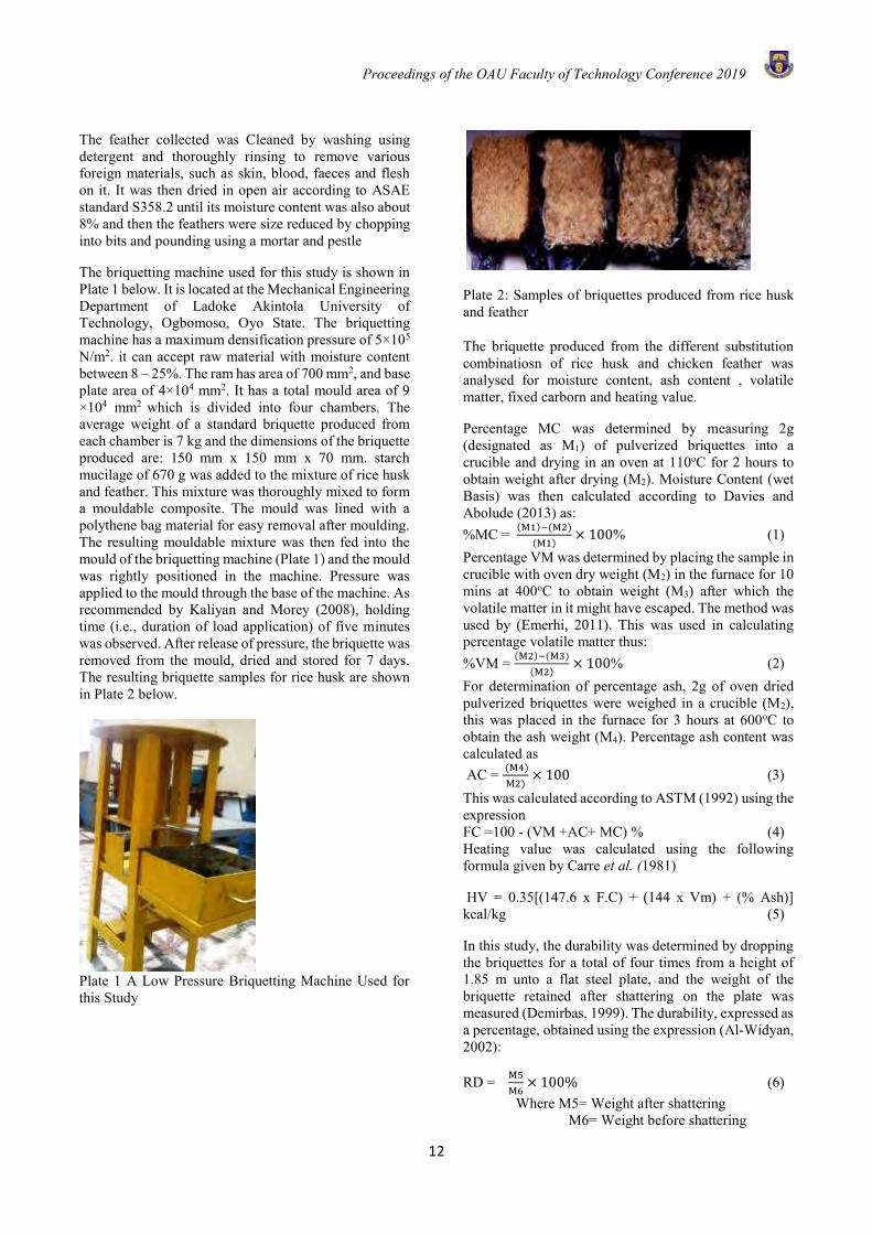
The briquetting machine used for this study is shown in Plate 1 below. It is located at the Mechanical Engineering Department of Ladoke Akintola University of Technology, Ogbomoso, Oyo State. The briquetting machine has a maximum densification pressure of 5×10⁵
N/m2. it can accept raw material with moisture content between 8 – 25%. The ram has area of 700 mm2, and base plate area of 4×104 mm2. It has a total mould area of 9 ×104 mm2 which is divided into four chambers. The average weight of a standard briquette produced from each chamber is 7 kg and the dimensions of the briquette produced are: 150 mm x 150 mm x 70 mm. starch mucilage of 670 g was added to the mixture of rice husk and feather. This mixture was thoroughly mixed to form a mouldable composite. The mould was lined with a polythene bag material for easy removal after moulding. The resulting mouldable mixture was then fed into the mould of the briquetting machine (Plate 1) and the mould was rightly positioned in the machine. Pressure was applied to the mould through the base of the machine. As recommended by Kaliyan and Morey (2008), holding time (i.e., duration of load application) of five minutes was observed. After release of pressure, the briquette was removed from the mould, dried and stored for 7 days. The resulting briquette samples for rice husk are shown in Plate 2 below.
Plate 1 A Low Pressure Briquetting Machine Used for this Study
Plate 2: Samples of briquettes produced from rice husk and feather
The briquette produced from the different substitution combinatiosn of rice husk and chicken feather was analysed for moisture content, ash content , volatile matter, fixed carborn and heating value.
Percentage MC was determined by measuring 2g (designated as M1) of pulverized briquettes into a crucible and drying in an oven at 110oC for 2 hours to obtain weight after drying (M2). Moisture Content (wet Basis) was then calculated according to Davies and Abolude (2013) as: %MC = (M1)−(M2)
(M1)× 100% (1)
Percentage VM was determined by placing the sample in crucible with oven dry weight (M2) in the furnace for 10 mins at 400oC to obtain weight (M3) after which the volatile matter in it might have escaped. The method was used by (Emerhi, 2011). This was used in calculating percentage volatile matter thus: %VM = (M2)−(M3)
(M2)× 100% (2)
For determination of percentage ash, 2g of oven dried pulverized briquettes were weighed in a crucible (M2), this was placed in the furnace for 3 hours at 600oC to obtain the ash weight (M4). Percentage ash content was calculated as AC = (M4)
M2)× 100 (3)
This was calculated according to ASTM (1992) using the expression FC =100 - (VM +AC+ MC) % (4) Heating value was calculated using the following formula given by Carre et al. (1981)
HV = 0.35[(147.6 x F.C) + (144 x Vm) + (% Ash)] kcal/kg (5)
In this study, the durability was determined by dropping the briquettes for a total of four times from a height of 1.85 m unto a flat steel plate, and the weight of the briquette retained after shattering on the plate was measured (Demirbas, 1999). The durability, expressed as a percentage, obtained using the expression (Al-Widyan, 2002):
RD = M5
M6× 100% (6)
Where M5= Weight after shattering M6= Weight before shattering
Proceedings of the OAU Faculty of Technology Conference 2019
13
The water resistance of the briquettes in this study was determined by recording the time the briquettes took to be fully immersed in tap water at room temperature (Kaliyan and Morey, 2008).
To determine the briquette density, A briquette sample was randomly selected and length, breadth, width of the briquette was measured using a meter rule. The volume was calculated thereafter (Vb). The weight of the briquette (M) was also determined using a digital weighing balance. Density of briquettes was calculated using the formula by ASTM (2004):
ꝭ = (M7)
(Vb) Kg/m3 (7)
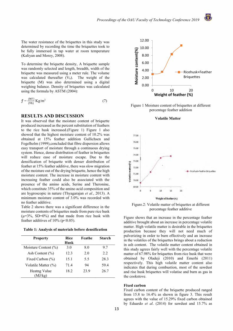
RESULTS AND DISCUSSION It was observed that the moisture content of briquette produced increased as the percent substitution of feathers to the rice husk increased.(Figure 1) Figure 1 also showed that the highest moisture content of 10.2% was obtained at 15% feather addition Gullichsen and Fogelholm (1999),concluded that fibre dispersion allows easy transport of moisture through a continuous drying system. Hence, dense distribution of feather in briquettes will reduce ease of moisture escape. Due to the densification of briquette with denser distribution of feather at 15% feather additive, there was slow migration of the moisture out of the drying briquette, hence the high moisture content. The increase in moisture content with increasing feather could also be associated with the presence of the amino acids, Serine and Theronine, which constitute 35% of the amino acid composition and are hygroscopic in nature (Thyagarajan et al., 2013). A minimum moisture content of 3.0% was recorded with no feather additive. Table 2 shows there was a significant difference in the moisture contents of briquettes made from pure rice husk (µ=3%, SD=0%) and that made from rice husk with feather additives of 10% (p<0.05).
Table 1: Analysis of materials before densification
Figure 1 Moisture content of briquettes at different percentage feather addition
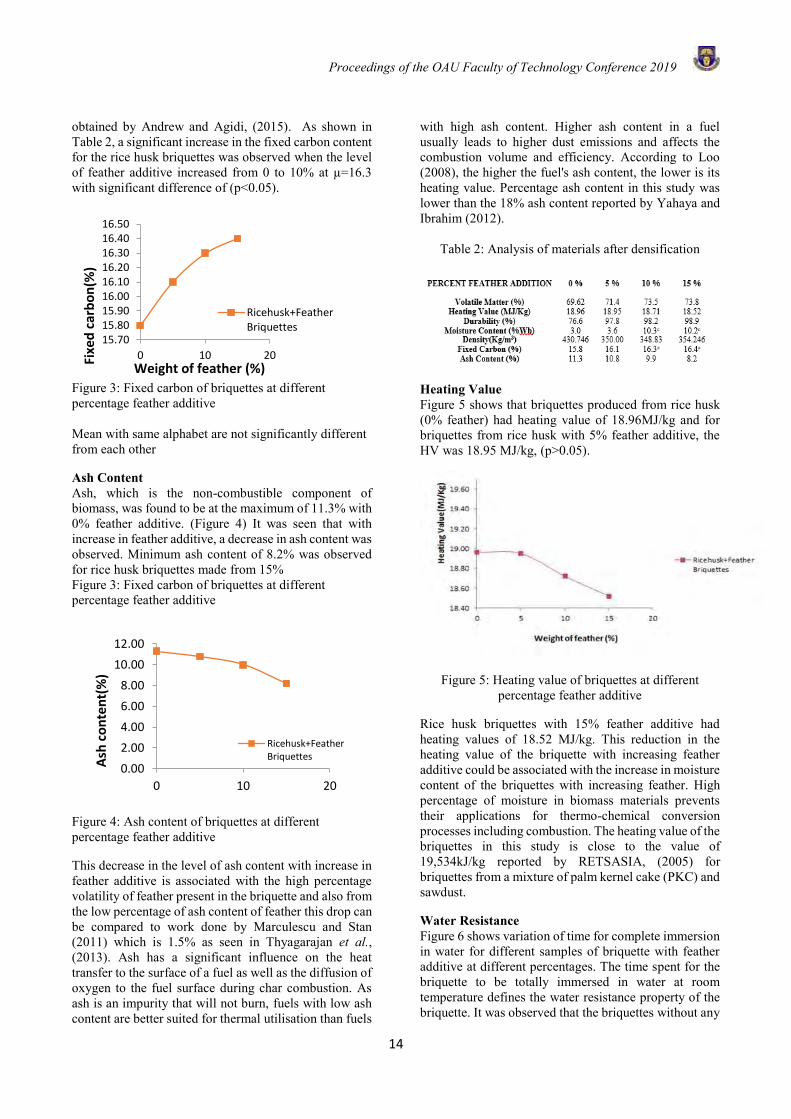
Volatile Matter
Figure.2: Volatile matter of briquettes at different
percentage feather additive
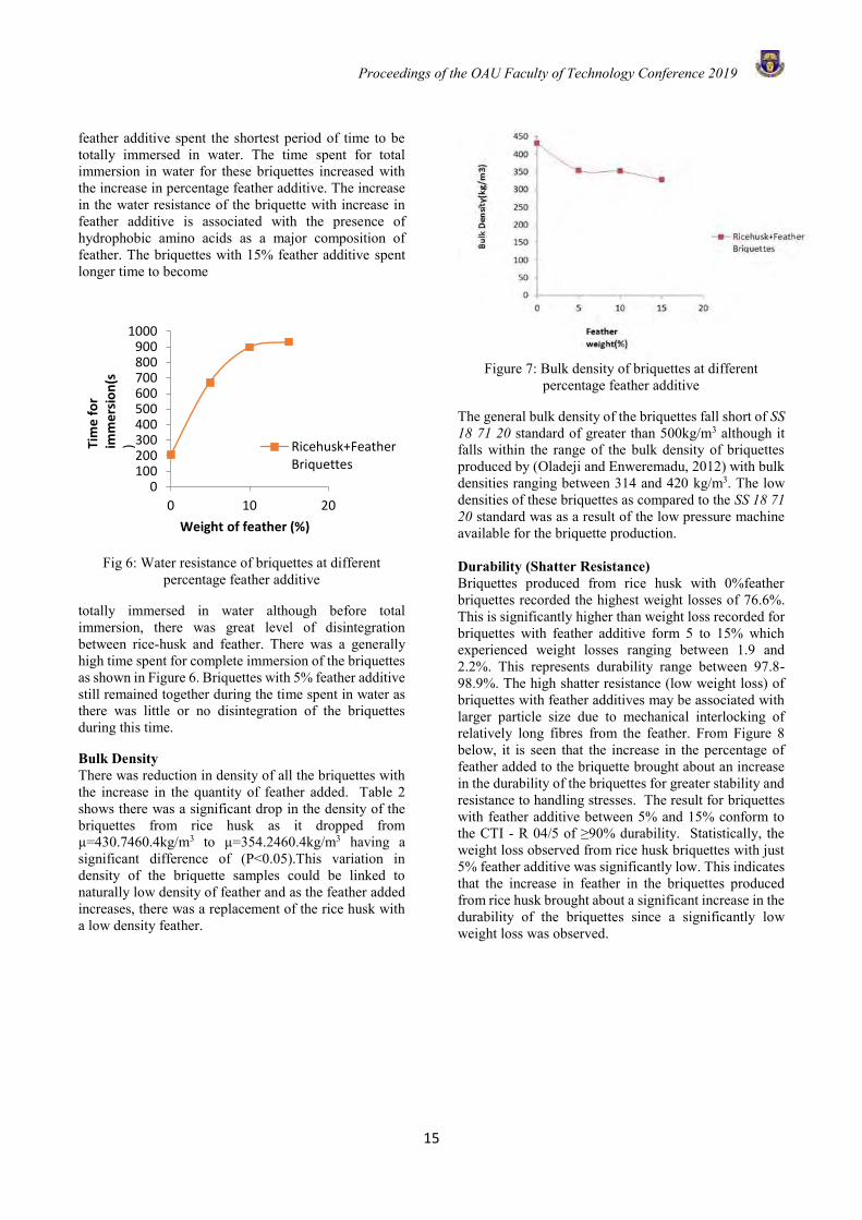
Figure shows that an increase in the percentage feather additive brought about an increase in percentage volatile matter. High volatile matter is desirable in the briquettes production because they will not need much of pulverizing in order to burn effectively and an increase in the volatiles of the briquettes brings about a reduction in ash content. The volatile matter content obtained in this study agrees fairly well with the percentage volatile matter of 67.98% for briquettes from rice husk that were obtained by Oladeji (2010) and Emerhi (2011) respectively. This high volatile matter content also indicates that during combustion, most of the sawdust and rise husk briquettes will volatise and burn as gas in the cookstove. Fixed carbon Fixed carbon content of the briquette produced ranged from 15.8 to 16.4% as shown in figure 3. This result agrees with the value of 15.29% fixed carbon obtained by Eduardo et al. (2014) for sawdust and 15.7% as
0.00
2.00
4.00
6.00
8.00
10.00
12.00
0 10 20
Ricehusk+FeatherBriquettes
Mo
istu
re c
on
ten
t(%
)
Weight of feather (%)
Property Rice Husk
Feathe Starch
Moisture Content (%) 3.0 8.0 9.7 Ash Content (%) 12.3 2.0 2.2 Fixed Carbon (%) 15.1 5.5 28.3
Volatile Matter (%) 71.4 94 59.4 Heatng Value
(MJ/kg) 18.2 23.9 26.7
Proceedings of the OAU Faculty of Technology Conference 2019
14
obtained by Andrew and Agidi, (2015). As shown in Table 2, a significant increase in the fixed carbon content for the rice husk briquettes was observed when the level of feather additive increased from 0 to 10% at µ=16.3 with significant difference of (p<0.05).
Figure 3: Fixed carbon of briquettes at different percentage feather additive Mean with same alphabet are not significantly different from each other
Ash Content Ash, which is the non-combustible component of biomass, was found to be at the maximum of 11.3% with 0% feather additive. (Figure 4) It was seen that with increase in feather additive, a decrease in ash content was observed. Minimum ash content of 8.2% was observed for rice husk briquettes made from 15% Figure 3: Fixed carbon of briquettes at different percentage feather additive
Figure 4: Ash content of briquettes at different percentage feather additive
This decrease in the level of ash content with increase in feather additive is associated with the high percentage volatility of feather present in the briquette and also from the low percentage of ash content of feather this drop can be compared to work done by Marculescu and Stan (2011) which is 1.5% as seen in Thyagarajan et al., (2013). Ash has a significant influence on the heat transfer to the surface of a fuel as well as the diffusion of oxygen to the fuel surface during char combustion. As ash is an impurity that will not burn, fuels with low ash content are better suited for thermal utilisation than fuels
with high ash content. Higher ash content in a fuel usually leads to higher dust emissions and affects the combustion volume and efficiency. According to Loo (2008), the higher the fuel's ash content, the lower is its heating value. Percentage ash content in this study was lower than the 18% ash content reported by Yahaya and Ibrahim (2012).
Table 2: Analysis of materials after densification
Heating Value Figure 5 shows that briquettes produced from rice husk (0% feather) had heating value of 18.96MJ/kg and for briquettes from rice husk with 5% feather additive, the HV was 18.95 MJ/kg, (p>0.05).
Figure 5: Heating value of briquettes at different percentage feather additive
Rice husk briquettes with 15% feather additive had heating values of 18.52 MJ/kg. This reduction in the heating value of the briquette with increasing feather additive could be associated with the increase in moisture content of the briquettes with increasing feather. High percentage of moisture in biomass materials prevents their applications for thermo-chemical conversion processes including combustion. The heating value of the briquettes in this study is close to the value of 19,534kJ/kg reported by RETSASIA, (2005) for briquettes from a mixture of palm kernel cake (PKC) and sawdust.
Water Resistance Figure 6 shows variation of time for complete immersion in water for different samples of briquette with feather additive at different percentages. The time spent for the briquette to be totally immersed in water at room temperature defines the water resistance property of the briquette. It was observed that the briquettes without any
15.7015.8015.9016.0016.1016.2016.3016.4016.50
0 10 20
Ricehusk+FeatherBriquettes
Weight of feather (%)
Fixe
dca
rbo
n(%
)
0.00
2.00
4.00
6.00
8.00
10.00
12.00
0 10 20
Ricehusk+FeatherBriquettes
Weight of
Ash
co
nte
nt(
%)
Proceedings of the OAU Faculty of Technology Conference 2019
15
feather additive spent the shortest period of time to be totally immersed in water. The time spent for total immersion in water for these briquettes increased with the increase in percentage feather additive. The increase in the water resistance of the briquette with increase in feather additive is associated with the presence of hydrophobic amino acids as a major composition of feather. The briquettes with 15% feather additive spent longer time to become
Fig 6: Water resistance of briquettes at different percentage feather additive
totally immersed in water although before total immersion, there was great level of disintegration between rice-husk and feather. There was a generally high time spent for complete immersion of the briquettes as shown in Figure 6. Briquettes with 5% feather additive still remained together during the time spent in water as there was little or no disintegration of the briquettes during this time.
Bulk Density There was reduction in density of all the briquettes with the increase in the quantity of feather added. Table 2 shows there was a significant drop in the density of the briquettes from rice husk as it dropped from µ=430.7460.4kg/m3 to µ=354.2460.4kg/m3 having a significant difference of (P<0.05).This variation in density of the briquette samples could be linked to naturally low density of feather and as the feather added increases, there was a replacement of the rice husk with a low density feather.
Figure 7: Bulk density of briquettes at different
percentage feather additive
The general bulk density of the briquettes fall short of SS 18 71 20 standard of greater than 500kg/m3 although it falls within the range of the bulk density of briquettes produced by (Oladeji and Enweremadu, 2012) with bulk densities ranging between 314 and 420 kg/m3. The low densities of these briquettes as compared to the SS 18 71 20 standard was as a result of the low pressure machine available for the briquette production. Durability (Shatter Resistance) Briquettes produced from rice husk with 0%feather briquettes recorded the highest weight losses of 76.6%. This is significantly higher than weight loss recorded for briquettes with feather additive form 5 to 15% which experienced weight losses ranging between 1.9 and 2.2%. This represents durability range between 97.8- 98.9%. The high shatter resistance (low weight loss) of briquettes with feather additives may be associated with larger particle size due to mechanical interlocking of relatively long fibres from the feather. From Figure 8 below, it is seen that the increase in the percentage of feather added to the briquette brought about an increase in the durability of the briquettes for greater stability and resistance to handling stresses. The result for briquettes with feather additive between 5% and 15% conform to the CTI - R 04/5 of ≥90% durability. Statistically, the weight loss observed from rice husk briquettes with just 5% feather additive was significantly low. This indicates that the increase in feather in the briquettes produced from rice husk brought about a significant increase in the durability of the briquettes since a significantly low weight loss was observed.
0100200300400500600700800900
1000
0 10 20
Ricehusk+FeatherBriquettes
Weight of feather (%)
Tim
efo
r im
me
rsio
n(s
)
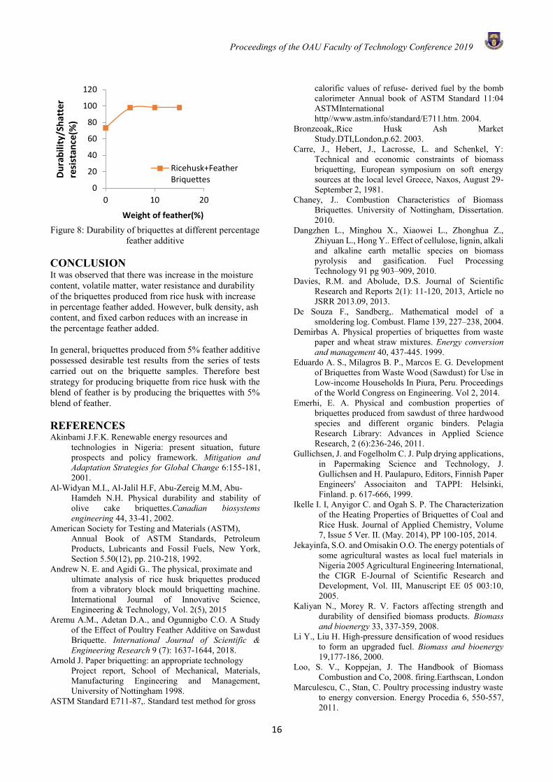
Proceedings of the OAU Faculty of Technology Conference 2019
16
Figure 8: Durability of briquettes at different percentage
feather additive CONCLUSION It was observed that there was increase in the moisture content, volatile matter, water resistance and durability of the briquettes produced from rice husk with increase in percentage feather added. However, bulk density, ash content, and fixed carbon reduces with an increase in the percentage feather added. In general, briquettes produced from 5% feather additive possessed desirable test results from the series of tests carried out on the briquette samples. Therefore best strategy for producing briquette from rice husk with the blend of feather is by producing the briquettes with 5% blend of feather. REFERENCES Akinbami J.F.K. Renewable energy resources and
technologies in Nigeria: present situation, future prospects and policy framework. Mitigation and Adaptation Strategies for Global Change 6:155-181, 2001.
Al-Widyan M.I., Al-Jalil H.F, Abu-Zereig M.M, Abu- Hamdeh N.H. Physical durability and stability of olive cake briquettes.Canadian biosystems engineering 44, 33-41, 2002.
American Society for Testing and Materials (ASTM), Annual Book of ASTM Standards, Petroleum Products, Lubricants and Fossil Fuels, New York, Section 5.50(12), pp. 210-218, 1992.
Andrew N. E. and Agidi G.. The physical, proximate and ultimate analysis of rice husk briquettes produced from a vibratory block mould briquetting machine. International Journal of Innovative Science, Engineering & Technology, Vol. 2(5), 2015
Aremu A.M., Adetan D.A., and Ogunnigbo C.O. A Study of the Effect of Poultry Feather Additive on Sawdust Briquette. International Journal of Scientific & Engineering Research 9 (7): 1637-1644, 2018.
Arnold J. Paper briquetting: an appropriate technology Project report, School of Mechanical, Materials, Manufacturing Engineering and Management, University of Nottingham 1998.
ASTM Standard E711-87,. Standard test method for gross
calorific values of refuse- derived fuel by the bomb calorimeter Annual book of ASTM Standard 11:04 ASTMInternational http//www.astm.info/standard/E711.htm. 2004.
Bronzeoak,.Rice Husk Ash Market Study.DTI,London,p.62. 2003.
Carre, J., Hebert, J., Lacrosse, L. and Schenkel, Y: Technical and economic constraints of biomass briquetting, European symposium on soft energy sources at the local level Greece, Naxos, August 29-September 2, 1981.
Chaney, J.. Combustion Characteristics of Biomass Briquettes. University of Nottingham, Dissertation. 2010.
Dangzhen L., Minghou X., Xiaowei L., Zhonghua Z., Zhiyuan L., Hong Y.. Effect of cellulose, lignin, alkali and alkaline earth metallic species on biomass pyrolysis and gasification. Fuel Processing Technology 91 pg 903–909, 2010.
Davies, R.M. and Abolude, D.S. Journal of Scientific Research and Reports 2(1): 11-120, 2013, Article no JSRR 2013.09, 2013.
De Souza F., Sandberg,. Mathematical model of a smoldering log. Combust. Flame 139, 227–238, 2004.
Demirbas A. Physical properties of briquettes from waste paper and wheat straw mixtures. Energy conversion and management 40, 437-445. 1999.
Eduardo A. S., Milagros B. P., Marcos E. G. Development of Briquettes from Waste Wood (Sawdust) for Use in Low-income Households In Piura, Peru. Proceedings of the World Congress on Engineering. Vol 2, 2014.
Emerhi, E. A. Physical and combustion properties of briquettes produced from sawdust of three hardwood species and different organic binders. Pelagia Research Library: Advances in Applied Science Research, 2 (6):236-246, 2011.
Gullichsen, J. and Fogelholm C. J. Pulp drying applications, in Papermaking Science and Technology, J. Gullichsen and H. Paulapuro, Editors, Finnish Paper Engineers' Associaiton and TAPPI: Helsinki, Finland. p. 617-666, 1999.
Ikelle I. I, Anyigor C. and Ogah S. P. The Characterization of the Heating Properties of Briquettes of Coal and Rice Husk. Journal of Applied Chemistry, Volume 7, Issue 5 Ver. II. (May. 2014), PP 100-105, 2014.
Jekayinfa, S.O. and Omisakin O.O. The energy potentials of some agricultural wastes as local fuel materials in Nigeria 2005 Agricultural Engineering International, the CIGR E-Journal of Scientific Research and Development, Vol. III, Manuscript EE 05 003:10, 2005.
Kaliyan N., Morey R. V. Factors affecting strength and durability of densified biomass products. Biomass and bioenergy 33, 337-359, 2008.
Li Y., Liu H. High-pressure densification of wood residues to form an upgraded fuel. Biomass and bioenergy 19,177-186, 2000.
Loo, S. V., Koppejan, J. The Handbook of Biomass Combustion and Co, 2008. firing.Earthscan, London
Marculescu, C., Stan, C. Poultry processing industry waste to energy conversion. Energy Procedia 6, 550-557, 2011.
0
20
40
60
80
100
120
0 10 20
Ricehusk+FeatherBriquettes
Weight of feather(%)
Du
rab
ility
/Sh
atte
rre
sist
ance
(%)

Proceedings of the OAU Faculty of Technology Conference 2019
17
Oladeji, J.T. Fuel Characterization of Briquettes produced from Corncob and Rice Husk Residue. Pacific Journal of Science and Technology, Vol. 11(1):101-106, 2010.
Oladeji J. T. and Enweremadu C. C. The Effects of Some Processing Parameters on Physical and Densification Characteristics of Corncob Briquettes. International Journal of Energy Engineering 2(1): 22-27, 2012.
Relova I., Vignote S., León M. A., Ambrosio Y.. Optimisation of the manufacturing variables of sawdust pellets from the bark of Pinus caribaea Morelet: Particle size, moisture and pressure. Biomass and Bioenergy, 33:1351-1357, 2009.
Proceedings of the OAU Faculty of Technology Conference 2019
18
AN ASSESSMENT OF THE FACTORS INFLUENCING THE ADOPTION OF EDUCATIONAL MANAGEMENT INFORMATION SYSTEM IN SELECTED
UNIVERSITIES IN SOUTHWESTERN NIGERIA
T.O. Akinwole1, T.O. Oyebisi1 and O.S. Ayanlade1,* 1African Institute for Science Policy and Innovation (AISPI),
Obafemi Awolowo University, Ile-Ife, Nigeria
*Email of Corresponding Author: [email protected]
ABSTRACT Due to the low adoption of Educational Management Information System, EMIS in Nigeria, this study aims at examining the factors influencing its adoption in selected universities in Southwestern zone of Nigeria. Both quantitative and qualitative methods were used in this study. Quantitatively, three hundred copies of questionnaire were administered among the students and staff (technology users) of the selected educational institutions using the EMIS technology, and also among EMIS officers at the ministry of education in each of the states of the zone. Qualitatively, semi-structured interviews were conducted at each selected university on one ICT staff, and also on one EMIS officer at the ministry of education of the states. Twenty-seven factors were presented to the respondents, gotten from the literature and the pilot study, measured on a likert scale of 1 (Strongly Disagree) to 5 (Strongly Agree). However using mean and Factor Analysis, six major factors were extracted, which were Lack of required users’ skills and competencies (4.43); Untimely communication among the institutions’ stakeholders (4.26); Institutional size (4.19); Lack of access to modern computing and communication technology, due to funds (4.13); Lack of users’ acceptance of the technology (4.10); and Unfavorable political structure of the government (3.90). The study therefore concluded, among others, because of the known benefits of EMIS, that there is a need for the government, institutions and other stakeholders of educational institutions, to provide or subsidize the needed fund, and also organize needed training and re-training for the users, to enhance skills acquisition. Keywords: Educational Management Information System, Adoption, Factor Analysis, Nigeria
INTRODUCTION Information is the basis of management, planning and evaluation of any organization, and educational organizations are not exemptions (UNESCO, 2017). If the relevant information required in a decision-making process or an organization planning is not available at the appropriate time, then there will be poor organizational planning, inappropriate decision-making, poor priority of needs, and defective programming or scheduling of activities (Adebayo, 2007).
Thus, Management Information System (MIS) is an aspect of information technology that assists the management of an organisation or enterprise in capturing, processing, storage and retrieval of relevant, up-to-date, and demand driven data and information, for optimal management functions (De Silva and Valsangkar, 2015).
Education has been proven to be a weapon for the development of attitudes and values which are capable of building a nation (Ajegbomogun and Salaam, 2011). It has generally been accepted as an instrument of change and effective tool for socioeconomic development. Also, it is the only weapon that has already been known for the achievement of persistent human development objectives in this era (Ojile and Tijani, 2017). According to UNESCO (2010a), school data and information of an educational system are very important, as they can be
used in financial planning, improving exam performance, instilling discipline, nurturing the students’ talents, make a standard comparism with other schools, help in reporting to authorities, assists in minimizing the wastage of students’ time as well as making the school projections among others. However, educational environment is collaborative i.e 'share data and information‘, because there are managers, policy makers, teachers, and students etc. This certainly demands the exchange and sharing of vital information especially in Nigeria, where the sector experiences high rate of growth (Mohamed et al., 2009). This is necessary because educational policy and decision-makers, and other educational planning managers need clear, easy to interpret comprehensible documents, accompanied by relevant analyses on which to base their decisions (UNESCO, 2017).
Thus, Educational Management Information System, EMIS, which is a special-purpose system, is useful in achieving management objectives by supplying appropriate and high quality information to its users for effective decision making (Karim, 2011). In other words, EMIS is a way of informing the different educational stakeholders (teachers, students, ministry of education etc), its internal and external efficiency, its pedagogical and institutional operations, its performance, shortcomings and needs (UNESCO, 2017). Furthermore, an EMIS is an organised group of information and
Proceedings of the OAU Faculty of Technology Conference 2019
19
documentation services that collects, stores processes analyzes and disseminates information for educational planning and management (UNDP, 2016). EMIS is also defined as “a system of people, technology, models, methods, processes, procedures, rules and regulations that function together to provide education leaders, decision makers and managers at all levels with a comprehensive, integrated set of relevant, reliable, unambiguous, and timely data and information to support them in completion of their responsibilities” (Kornkaew, 2012).
An EMIS thus has a function to collect and analyze management indicators related to the educational sector, and aims to support the processes of strategic planning, resource assignation, monitoring, policy formulation and decision making in institutions of Higher Education (UNESCO, 2010b). De Silva and Valsangkar (2015) stated some types and examples of EMIS according to some key areas that EMIS is useful in decision making. These include Students’ Management Information System; Teachers’ Management Information System; School Management Information System; Infrastructure Management Information System; Asset Management Information System; Classroom Management Information System and National Learning Assessment.
Therefore, several authors have explored that the critical information required by midlevel and strategic level management in educational sector is efficiently provided by EMIS (Moore, 2005). However, decision making may be difficult when there is information overload, that is, large information available to be used by managers, so the needed information must be simply, precise and timely available. The resourceful use of information thus makes reliable decision making possible (Aldarbesti and Saxena, 2014).
However, due to the low adoption of Educational Management Information System, EMIS in Nigerian educational sector, this study aims at examining the factors influencing its adoption in selected universities in Southwestern zone of Nigeria.
MATERIALS AND METHODS This study was conducted in Nigeria, in the Southwestern geopolitical zone, which comprises of Osun, Oyo, Lagos, Ogun, Ekiti and Ondo states. According to the National Universities Commission, NUC (2018), there were a total of 170 universities in Nigeria and these comprise 43 federal, 48 state and 79 private universities. However, the study purposively targeted six (6) universities in Nigeria that have already adopted Educational Management Information System (EMIS), and also involved EMIS departments of ministry of education in each of the states in southwestern Nigeria. Both quantitative and qualitative methods were used in this study. In other words, primary data was collected using structured questionnaire, while also supplemented with semi structured interviews. Quantitatively, three hundred (300) copies of questionnaire were administered among
the students and staff (EMIS users) of the selected educational institutions, and also among EMIS officers at the ministry of education also in each of the states of the zone. Qualitatively, semi-structured interviews were conducted at each selected university on one ICT staff, and also on one EMIS officer at the ministry of education of the states.
Therefore, the population of the study comprised the school management, students and ICT Staff (who are the users of the EMIS), in the selected universities and EMIS officers in the state ministries of education. In each of the university selected, random sampling was used to select the respondents who filled the questionnaire. The respondents (students and ICT staffs) were selected for the study because they were the major users: they use the system regularly, while the school managements in the selected universities are involved in the administration of the various schools, and thus would supposedly give reliable responses for this study. At the ministry of education offices, random sampling was also used to select the EMIS officers who participated in the study, as they are involved in giving information about the educational sector to the government. Thus, three (3) sets of questionnaire were designed: One set for 5 respondents of each school management staff (making 30 respondents in all the six states); Another set for 10 staff and 30 students from each school using the Educational Management Information System (thus 60 staff and 180 students from the six states); finally the last set was for 5 Staff of the State Ministry of Education (making 30 respondents in all the six states). Therefore, a total of three hundred (300) copies of questionnaire altogether were administered for the study. Furthermore, a semi structured interview was carried out with one (1) ICT staff in each school and one (1) EMIS officer in each ministry of Education.
RESULTS AND DISCUSSION Factors Influencing Adoption of Educational Management Information System (EMIS) in the Institutions: Quantitative Results
Altogether, out of 300 copies of questionnaires administered, 289 were able to be retrieved. Therefore, the response rate was 96.3%. Twenty-seven factors that influence adoption of EMIS options in the Southwestern states institutions in Nigeria were presented to the respondents, gotten from the literature and the pilot study conducted for the study, measured on a likert scale of 1 (Strongly Disagree) to 5 (Strongly Agree) as shown in Table 1. However using mean and Factor Analysis, six major factors were extracted from the presented factors to show the most important factors, which were Lack of required users’ skills and competencies (4.43); Untimely communication among the institutions’ stakeholders (4.26); Institutional size (4.19); Lack of access to modern computing and communication technology due to funds (4.13); Lack of users’ acceptance of the technology (4.10); and Unfavorable political structure of the government (3.90).
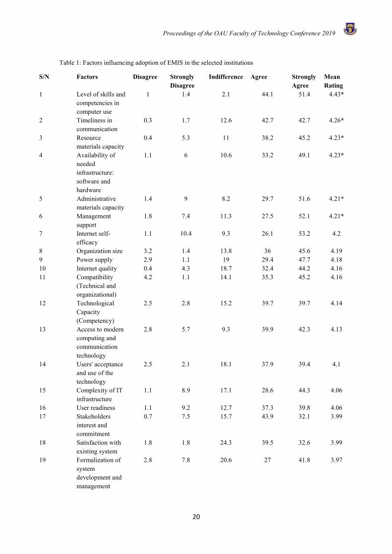
Proceedings of the OAU Faculty of Technology Conference 2019
20
Table 1: Factors influencing adoption of EMIS in the selected institutions
S/N Factors Disagree Strongly Disagree
Indifference Agree Strongly Agree
Mean Rating
1 Level of skills and competencies in computer use
1 1.4 2.1 44.1 51.4 4.43*
2 Timeliness in communication
0.3 1.7 12.6 42.7 42.7 4.26*
3 Resource materials capacity
0.4 5.3 11 38.2 45.2 4.23*
4 Availability of needed infrastructure: software and hardware
1.1 6 10.6 33.2 49.1 4.23*
5 Administrative materials capacity
1.4 9 8.2 29.7 51.6 4.21*
6 Management support
1.8 7.4 11.3 27.5 52.1 4.21*
7 Internet self-efficacy
1.1 10.4 9.3 26.1 53.2 4.2
8 Organization size 3.2 1.4 13.8 36 45.6 4.19 9 Power supply 2.9 1.1 19 29.4 47.7 4.18 10 Internet quality 0.4 4.3 18.7 32.4 44.2 4.16 11 Compatibility
(Technical and organizational)
4.2 1.1 14.1 35.3 45.2 4.16
12 Technological Capacity (Competency)
2.5 2.8 15.2 39.7 39.7 4.14
13 Access to modern computing and communication technology
2.8 5.7 9.3 39.9 42.3 4.13
14 Users' acceptance and use of the technology
2.5 2.1 18.1 37.9 39.4 4.1
15 Complexity of IT infrastructure
1.1 8.9 17.1 28.6 44.3 4.06
16 User readiness 1.1 9.2 12.7 37.3 39.8 4.06 17 Stakeholders
interest and commitment
0.7 7.5 15.7 43.9 32.1 3.99
18 Satisfaction with existing system
1.8 1.8 24.3 39.5 32.6 3.99
19 Formalization of system development and management
2.8 7.8 20.6 27 41.8 3.97
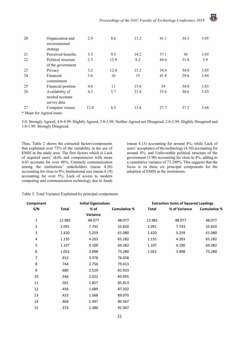
Proceedings of the OAU Faculty of Technology Conference 2019
21
20 Organization and environmental strategy
2.9 8.6 13.2 41.1 34.3 3.95
21 Perceived benefits 3.3 9.5 14.2 37.1 36 3.93 22 Political structure
of the government 2.5 12.9 8.2 44.6 31.8 3.9
23 Privacy 3.2 12.4 15.2 34.4 34.8 3.85 24 Financial
commitment 3.6 10 15 41.8 29.6 3.84
25 Financial position 4.6 11 15.6 34 34.8 3.83 26 Availability of
needed accurate survey data
4.3 5.7 23.8 35.6 30.6 3.83
27 Computer viruses 12.8 8.5 13.8 27.7 37.2 3.68 * Mean for Agreed items
5.0: Strongly Agreed, 4.0-4.99: Slightly Agreed, 3.0-3.99: Neither Agreed nor Disagreed, 2.0-2.99: Slightly Disagreed and 1.0-1.99: Strongly Disagreed.
Thus, Table 2 shows the extracted factors/components that explained over 73% of the variability in the use of EMIS in the study area. The first factors which is Lack of required users’ skills and competencies with mean 4.43 accounts for over 48%; Untimely communication among the institutions’ stakeholders (mean 4.26) accounting for close to 8%; Institutional size (mean 4.19) accounting for over 5%; Lack of access to modern computing and communication technology due to funds
(mean 4.13) accounting for around 4%; while Lack of users’ acceptance of the technology (4.10) accounting for around 4%; and Unfavorable political structure of the government (3.90) accounting for close to 4%, adding to a cumulative variance of 73.280%. This suggests that the focus is on these six principal components for the adoption of EMIS in the institutions.
Table 2: Total Variance Explained by principal components
Component Initial Eigenvalues Extraction Sums of Squared Loadings
S/N Total % of
Variance
Cumulative % Total % of Variance Cumulative %
1 12.981 48.077 48.077 12.981 48.077 48.077
2 2.091 7.743 55.820 2.091 7.743 55.820
3 1.420 5.259 61.080 1.420 5.259 61.080
4 1.135 4.203 65.282 1.135 4.203 65.282
5 1.107 4.100 69.382 1.107 4.100 69.382
6 1.052 3.898 73.280 1.052 3.898 73.280
7 .912 3.378 76.658
8 .744 2.756 79.413
9 .680 2.519 81.933
10 .546 2.022 83.955
11 .501 1.857 85.813
12 .456 1.689 87.502
13 .423 1.568 89.070
14 .404 1.497 90.567
15 .373 1.380 91.947
Proceedings of the OAU Faculty of Technology Conference 2019
22
16 .345 1.279 93.227
17 .294 1.088 94.314
18 .252 .934 95.249
19 .216 .799 96.048
20 .202 .747 96.795
21 .195 .724 97.519
22 .155 .574 98.092
23 .142 .528 98.620
24 .129 .479 99.099
25 .102 .376 99.475
26 .082 .304 99.779
27 .060 .221 100.000
Qualitative Result and Discussion of Interview Data on Factors Influencing Adoption of Educational Management Information System (EMIS) in the Institutions In the similar vein, the qualitative approach examined respondents’ views about the factors that possibly influence the adoption of EMIS in the institutions. The main themes that came out in the interview were lack of needed skills and competencies; lack of access to other modern computing and communication technology; uninterruptible power supply; lack of availability of needed infrastructure; lack of quality and good access to internet; low user’s acceptance and readiness for technology use; lack of satisfaction on the existing system, among others.
Some of the responses included for examples: A married female respondent with 15 years of working experience were opined that skills and competencies among others would enable institutions to adopt the use of EMIS option. According to her:
“There are many factors that would affect the use of EMIS in any work place, but the level of skills and competencies in computer use is one of the basic factors, and timeliness in communication as well as access to other modern computing and communication technology. I will also mention uninterruptible power supply and availability of needed infrastructure are inevitable factors………..”
Similarly, a married male above 40 years old mentioned that reiterated skills and level of technological know-how, to mention but afew, influence the adoption of EMIS in Nigerian universities. According to him:
“……. there are many factors, the major influencing factors are resources capacity, access to modern computing, quality and good access to internet. Others I will like to say are
user’s acceptance on technology use, satisfaction on existing system and others”.
A married male of aged 40 years was of the opinion that access to internet facility and the interest of the stakeholders would enable the institutions to adopt EMIS. According to him:
“To me, timeliness in communication, access to modern computing and communication technology, stakeholders’ interest and commitment, as well as quality internet would influence adoption of EMIS technology”.
CONCLUSION
The study showed that the main factors influencing the adoption of EMIS in the study area are Lack of required users’ skills and competencies; Untimely communication among the institutions’ stakeholders; Institutional size; Lack of access to modern computing and communication technology, due to funds; Lack of users’ acceptance of the technology; and Unfavorable political structure of the government.
The study therefore concluded, among others, because of the known benefits of EMIS, that there is a need for the government, institutions and other stakeholders of educational institutions, to provide or subsidize the needed software and hardware for EMIS, and also organize training and re-training for the users, to enhance skills acquisition.
REFERENCES
Adebayo, F. A. (2007). Management information system for managers. Ado-Ekiti: Green Line Publishers
Ajegbomogun F. O. and Salaam M. O. (2011). “The State of School Libraries in Nigeria”, PNLA Quarterly, the official publication of the Pacific Northwest Library Association Volume 75, no. 3 (Spring 2011). Available at:

Proceedings of the OAU Faculty of Technology Conference 2019
23
https://www.academia.edu/3253775/The_State_of_School_Libraries_in_Nigeria
Aldarbesti H., and Saxena J. P., (2014). “Management Information System for Education” e-ISSN: 2320–7388, p-ISSN: 2320–737X. Vol. 4(1) pp. 36-44
De Silva, S. and Valsangkar, P. 2015. The impact of education management information systems: the case of Afghanistan]. Available at: http://blogs.worldbank.org/education/impacteducation-management-information-systems-case-
Karim, A. J. (2011). The significance of management information systems for enhancing strategic and tactical planning. JISTEM-Journal of Information Systems and Technology Management, vol. 8(2), pp. 459-470.
Kornkaew A., (2012). “Management Information System Implementation Challenges, Success Key Issues, Effects and Consequences. A Case Study of Fenix System”. Master’s Thesis within Military Logistics, Jönköping University.
Moore K., (2005). “Administrative Barriers to Adoption of Distance Education”. [Online] Available at: http://www.knight-moore.com/pubs/ajde 8-3.html
National Universities Commission NUC (2018), “List of universities in Nigeria as approved by the NUC, 2018”, available at: http://nuc.edu.ng
Ojile E. A. and Tijani O. A. (2017). “EDUCATION FOR SUSTAINABLE ECONOMIC DEVELOPMENT IN NIGERIA: THE CONTENDING ISSUES” Journal of Faculty of Education, University of Calabar, Calabar – Nigeria, Education For Today, Vol. 13(1), pp. 95-97
United Nations Development Program UNDP (2016). Human Development Report – Human Development for Everyone. NewYork: UNDP
UNESCO, 2010a. “UNESCO National Education Support Strategy (UNESS) for the Republic of Kenya 2010 – 2011”, UNON, Nairobi-Kenya.
UNESCO, 2010b. “Guidebook for planning education in emergencies and reconstruction, Paris”: International Institute for Educational Planning, 2010: p. 2, available at: http://unesdoc.unesco.org/images/0019/001902/190223e.pdf
UNESCO, (2017). Leveraging Information and Communication Technology to Achieve
Education 2030. Report of the UNESCO 2017 International Forum on ICT and Education 2030. 10 – 11 July 2017, Qingdao, the People’s Republic of China.
Proceedings of the OAU Faculty of Technology Conference 2019
24
AN IMPROVED NETWORK CONGESTION AVOIDANCE MODEL
B. O. Akinyemi1,* and T. A. Adiatu2 12Department of Computer Science and Engineering
Obafemi Awolowo University, Ile-Ife
*Email of Corresponding Author: [email protected]
ABSTRACT Network scheduling as a mechanism to prevent network congestion usually reorders or drop network packets under overload. Packets from flows in the network that gets dropped are usually resent to prevent data loss or breakage, which may result in unnecessary buffering and bottleneck in the limited network bandwidth allocation, thus leading to congestion. Existing solutions mostly suffer from static implementation of avoidance mechanism with little or no consideration for bandwidth allocation fairness among communicating nodes. Thus, it is a dire technological need, a mechanism to efficiently and effectively mitigate this network congestion scenario. In this paper, a congestion avoidance model was developed by employing a combination of intelligent boundary policing mechanism and low complexity fairness enforcing scheme. Network Simulator 3 (NS-3) tools written in C++ and Python scripting interface were used to simulate the model formulated. The simulation output was presented as traced files and was animated using Netanim to produce the graph and tables. Performance evaluation results of the model showed that 88.24% (45 of 51 cases) packet was transferred successfully through the network, which implied lowered congestion possibility, high percentage stability, and very low algorithm complexity. The result of the simulation demonstrated that the proposed model optimizes bandwidth usage by 2%, minimizes the network latency by 4.5%, minimizes the packet loss by 10% and optimizes throughput through its low complexity fairness enforcing scheme. Keywords: Tele-congestion, Network Scheduling, Avoidance Mechanism INTRODUCTION A major issue in the quality of service of data network is network congestion. Network congestion occurs when provided traffic load transcends available capacity at any point in a network (Hull et al., 2004). It is a condition in which an increase in data transmissions gives rise in a reduction in network throughput. Network congestion is refer to the reduced Quality of Service (QoS) that happens when a node in a network conveys more data than it can actually handle. Some outcomes include blocking of new connections, packet loss or queueing delay. Significance of the former two outcomes is that an incremental increase in provided network load leads either only to a small decrease or even an increase in a network throughput (James et al., 2015). During the transfer of packets across the network, there is impending network failure which will have effect on the network throughput i.e. the amount of data to be transmitted. Retransmitting packets makes the throughput of the network to decrease and latency of the network to increase. Packet loss denotes the loss which occurs when one or more packets moving across a network connection failed to arrive at their destination. The higher the network throughput, the lower the packet loss, and the better is the performance of the network. Also, it is evident that the response time of a network is directly proportional to the capacity of the network. The response time is used to ascertain the latency of the network. The lower the response time, the lower the network latency and the other way around. The smaller the delay or latency, the better is the performance of the network. Packets can get lost for two reasons; it is either they are impaired while in transit, or the network is congested and
in a particular location on the route, there was an insufficient buffer capacity. On most network routes, loss due to impairment is rare (about <1%), so it is likely that a packet loss emanates from congestion in the network (Jacobson, 1988). Internet users are only concerned with the throughput and latency of the network they use. In internetworking, throughput is amount of the data that a network subscribers can draw from the network over time which is most evident in the communication of large files and latency refers to the period it takes a packet to travel from a server to a client which is most evident in the use of interactive applications. While the throughput increases on a network node or router, latency also increases owing to the growing network delay and the busty characteristics of the Transmission Control Protocol (TCP). Increase in latency which is proportional to increase in bandwidth is initially always marginal in networks but when the maximum achievable throughput is reached, latency begins to increase exponentially until it attains a final tipping point where the network elements experience congestion collapse. Hence, there comes a need to manage the activities of the network and network elements leading to congestion collapse. Informally, congestion collapse takes place when an increase in the network load results in a decrease in the Quality of Service (QoS) by the network (Floyd and Fall, 1999). Congestion management solutions usually have two operational components mechanisms. Firstly, a mechanism to ease the impact of congestion and secondly, a mechanism to switch on the ease mechanism. A complete congestion solution demands these two
Proceedings of the OAU Faculty of Technology Conference 2019
25
components, yet, available solutions based on this high-level view of congestion management vary tremendously in effectiveness and complexity. Networks employ congestion control and avoidance techniques to attempt to manage congestion collapse. Network congestion control is the congestion management scheme in which end systems eased off to avoid congesting the network. This method is similar to end-to-end flow controls, but the aim is to decrease congestion in the network and not the receiver. Network-based congestion avoidance is the scheme whereby a router discovers that congestion may occur and make efforts to slow down the senders before queues filled to capacity. A congestion avoidance strategy, also have two components: The network should indicate to the transport endpoints that congestion is occurring or not. Meanwhile, a policy that decreases utilization if this signal is received and increases utilization if the signal is not received is required by the endpoints (Jacobson, 1988). One method of congestion avoidance is packet dropping i.e. the discretional re-ordering or dropping of network packets under overload. The other method is the implementation of priority schemes, to transmit packets having higher priority than others. Another method is to explicitly allot network resources to specific flows. Commonly router congestion avoidance mechanisms are scheduling algorithms like fair queuing, and Random Early Detection (RED), whereby packets are randomly dropped, proactively activating the endpoints to slow down the transmission before congestion collapse occurs. Fair queuing is mostly utilized in routers at chokepoints with a small number of connections moving through them. Larger routers usually counts on RED. Noteworthy, the network protocols that employs aggressive retransmissions to counterbalance the effect of packet loss owing to congestion can also increase congestion, even after the initial network load has been reduced to a level that would not at least have induced network congestion (Radhadevi and Anjaneyulu, 2013). The primary foundation for congestion control in the Internet is the TCP congestion avoidance algorithm (Low et al., 2002). The technological need to prevent network failure or in the minimum increase the mean time between failures, eliminating congestion scenario in computer networks, intelligently and dynamically distributing network resources all justifies the need for the avoidance system. During peak hours, most organisation’s networks usually experienced congestion and the solution proffered will be to drop some network traffic and thus packets from flows in the network that gets dropped is usually resent to prevent data loss or breakage, consequently leading to unnecessary buffering and bottleneck in the limited bandwidth allocation of organisations resulting to congestion.
However, existing congestion protocols mostly suffers from the static implementation of avoidance mechanism with little or no consideration for bandwidth allocation fairness among communicating nodes. Since, end-to-end congestion control of best-effort traffic is necessitated to avoid the global Internet experiencing congestion collapse (Floyd and Fall, 1999). Hence, it is a dire technological need, a mechanism to efficiently and effectively mitigate this network congestion scenario. Thus, an attempt is made in this paper to reduce or eradicate the issues of network congestion, unfair bandwidth allocation causing bottlenecks and provide a new friendly platform for interconnecting devices to communicate. RELATED WORKS Congestion control in networks have been a recurring problem for many years. Various algorithms abound on congestion avoidance systems with different methodologies ranging from the TCP’s rate control mechanisms to the diverse congestion control mechanisms employed in the existing systems. The conduct of many end-to-end protocols is better under congested conditions. TCP is possibly the best-behaved. Since UDP do not have the capability to control congestion, protocols built at the top of the UDP must manage congestion independently. Also, protocols that are congestion-free and transmit at a fixed rate can be problematic. Real-time streaming protocols, including many VoIP (Voice over Internet Protocols), exhibits this property. Thus, standard procedures such as quality-of-service routing, has been employed to avoid packets being dropped. TCP uses a network congestion avoidance algorithm that considers various features of an Additive Increase/Multiplicative Decrease (AIMD) scheme, with some other schemes such as slow start and congestion window to accomplish congestion avoidance (Chiu and Jain, 1989, Floyd et al., 2000). The problem of congestion collapse experienced by early TCP/IP protocols has motivated the study of end-to-end congestion control algorithms in the late 1980s (Firoiu and Borden, 2000). However, end-to-end congestion control algorithms alone are ineffective to prevent the congestion collapse and unfairness brought about by applications that are unresponsive to network congestion. Random Early Detection (RED) gateway (Floyd and Jacobson, 1993) is an early example of mechanisms for congestion avoidance in packet-switched networks. This mechanism is comparatively a simple gateway algorithm that could be implemented in homogeneous networks because the RED gateway improves the fairness of homogeneous connections that have the same bottleneck, but beyond that, it has limited value because it only allows intentionally conceived design decisions to be made about the average queue size and maximum queue size allowed at the gateway. The weakness lies in finding
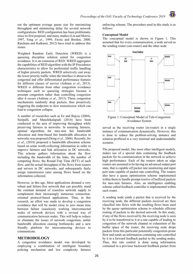
Proceedings of the OAU Faculty of Technology Conference 2019
26
out the optimum average queue size for maximizing throughput and minimizing delay for several network configurations. RED configuration has been problematic since its first proposal, and many studies (Lin and Morris, 1997, Feng et al., 1999, Firoiu and Borden, 2000, Raichana and Kulkarni, 2012) have tried to address this issues. Weighted Random Early Detection (WRED) is a queueing discipline solution suited for congestion avoidance. It is an extension of RED. WRED aggregates the capabilities of RED algorithm with the IP Precedence characteristics to allow for preferential traffic handling of higher priority packets. WRED selectively cast away the lower priority traffic when the interface is about to be congested and offer differentiated performance features for different classes of service (Ashima et al., 2013). WRED is different from other congestion avoidance techniques such as queueing strategies because it preempt congestion rather than controlling congestion after it occurs (Ashima et al., 2013). These congestion mechanisms randomly drop packets, thus proactively triggering the endpoints to slow transmission which can lead to congestion collapse. A number of researches such as Ee and Bajcsy (2004), Saripalli, and Manchikalapudi (2014) have been conducted in the area of improving throughput while preserving fairness in networks. In ensuring fairness, optimal algorithms for max-min fair bandwidth allocation and time-based fair bandwidth allocation in networks was proposed (Dong et al., 2006). Recently, Ito et al., (2018) proposed a bandwidth allocation scheme based on some worth-collecting information in order to improve fairness and link utilization in DC networks. This scheme gathers information about the flow including the bandwidth of the links, the number of competing flows, the Round-Trip Time (RTT) of each flow, and the actual throughput of the flows from routers and servers in DC networks, and subsequently fairly assign transmission rates among flows based on the information collected. However, in this age, Most applications demand a very robust and failure-free network that can possibly stand the constant demand of ceaseless network supply to complement their increasingly numerous connection-oriented protocol-based applications. Thus, in this research, an effort was made to develop a congestion avoidance that will be model close to zero mean time between failure ceaselessly working interconnected nodes of network devices with a revised way of communication between nodes. This will help to reduce or eliminate the issues of network congestion, unfair bandwidth allocation causing bottlenecks and a new friendly platform for interconnecting devices to communicate.
METHODOLOGY A congestion avoidance model was developed by employing a combination of intelligent boundary policing mechanism and low complexity fairness
enforcing scheme. The procedure used in this study is as follows: Conceptual Model The conceptual model is shown in Figure 1. This assumed that for every communication, a node served as the sending router (out-router) and the other node
Figure 1: Conceptual Model of Tele-Congestion
Avoidance System served as the receiving router (in-router) in a single instance of communication dynamically. However, this is done to reduce the problem-solving instance and solution proffered to a very minimal and understandable scenario. The proposed model, like most other intelligent models, makes use of a special data containing the feedback packets for its communication in the network to achieve high performance. Each of the routers taken as edge routers are assumed to be having an advanced output port state, that is capable off packet rate monitoring and input port state capable of packet rate controlling. The routers also have a queue optimization scheme implemented within them to handle prompt resolve of buffered packets for max-min fairness. Also, an intelligence enabling scheme called feedback controller is implemented within each router. A sending node sends a packet that is received by the receiving node, the different packets received are then classified into flows with the resulting flows been used by the queue optimization scheme to schedule efficient routing of packets to the desired network. In this study, if any of the flows received by the receiving node is seen by it to be transferred to it at a rate capable of leading to congestion of the network channel or exhaustion of the buffer space of the router, the receiving node drops packets from this particular potentially congestion-prone flow and sends an information containing rate controlled by it in a forward feedback packet to the sending nodes. Thus, this rate control is done using information contained in a previous backward feedback packet from
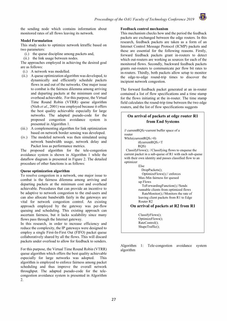
Proceedings of the OAU Faculty of Technology Conference 2019
27
the sending node which contains information about monitored rates of all flows leaving its network. Model Formulation This study seeks to optimize network ktraffic based on two parameters:
(i.) the queue discipline among packets and, (ii.) the link usage between nodes.
The approaches employed in achieving the desired goal are as follows:
(i.) A network was modelled. (ii.) A queue optimization algorithm was developed, to
dynamically and efficiently schedule packets flows in and out of the networks. One major issue to combat is the fairness dilemma among arriving and departing packets at the minimum cost and overhead achievable. For this purpose, the Virtual Time Round Robin (VTRR) queue algorithm (Nieh et al., 2001) was employed because it offers the best quality achievable especially for large networks. The adapted pseudo-code for the proposed congestion avoidance system is presented in Algorithm 1.
(iii.) A complementing algorithm for link optimization based on network border sensing was developed.
(iv.) The modeled network was then simulated using network bandwidth usage, network delay and Packet loss as performance metrics.
The proposed algorithm for the tele-congestion avoidance system is shown in Algorithm 1 while the dataflow diagram is presented in Figure 2. The detailed procedure of other functions is as follows: Queue optimization algorithm To resolve congestion in a network, one major issue to combat is the fairness dilemma among arriving and departing packets at the minimum cost and overhead achievable. Procedures that can provide an incentive to be adaptive to network congestion to the end-users and can also allocate bandwidth fairly in the gateways are vital for network congestion control. An existing approach employed by the gateway was per-flow queuing and scheduling. This existing approach can ascertain fairness, but it lacks scalability since many flows pass through the Internet gateway. In this research, in order to increase efficiency and reduce the complexity, the IP gateways were designed to employ a single First-In-First Out (FIFO) packet queue collaboratively shared by all the flows. This will discard packets under overload to allow for feedback to senders. For this purpose, the Virtual Time Round Robin (VTRR) queue algorithm which offers the best quality achievable especially for large networks was adopted. This algorithm is employed to enforce fairness among packet scheduling and thus improve the overall network throughput. The adapted pseudo-code for the tele-congestion avoidance system is presented in Algorithm 2.
Feedback control mechanism This mechanism checks how and the period the feedback packets are exchanged between the edge routers. In this research, feedback packets are taken as a form of an Internet Control Message Protocol (ICMP) packets and these are essential for the following reasons. Firstly, forward feedback packets grant in-routers to detect which out-routers are working as sources for each of the monitored flows. Secondly, backward feedback packets grants out-routers to communicate per flow bit rates to in-routers. Thirdly, both packets allow setup to monitor the edge-to-edge round-trip times to discover the incipient network congestion. The forward feedback packet generated at an in-router contained a list of flow specifications and a time stamp for the flows initiating at the in-router. The time stamp field calculates the round-trip time between the two edge routers, and the list of flow specifications suggests Algorithm 1: Tele-congestion avoidance system algorithm
On arrival of packets at edge router R1 from End Systems
// currentRQSi=current buffer space of a router While(currentRQS1>0)
if(currentRQS1<TRQS)
ClassifyFlows(); //Classifying flows to enqueue the current packet in a sub-queue of R1 with each sub-queue with their own identity and passes classified flow to an optimizer
Else DropPackets();
OptimizeFlows();// enforces Max-Min fairness for queued up Flows ToForwardingFunction();//Sends runnable clients from optimized flows RateMonitor();//Monitors the rate of leaving client packets from R1 to Edge Router R2
On arrival of packets at R2 from R1
ClassifyFlows(); OptimizeFlows(); RateControl(); ShapeTraffic();
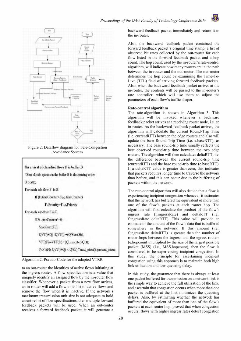
Proceedings of the OAU Faculty of Technology Conference 2019
28
Figure 2: Dataflow diagram for Tele-Congestion
Avoidance System
Algorithm 2: Pseudo-Code for the adapted VTRR to an out-router the identities of active flows initiating at the ingress router. A flow specification is a value that uniquely identify an assigned flow by the in-router flow classifier. Whenever a packet from a new flow arrives, an in-router will add a flow to its list of active flows and remove the flow when it is inactive. If the network’s maximum transmission unit size is not adequate to hold an entire list of flow specifications, then multiple forward feedback packets will be used. When an out-router receives a forward feedback packet, it will generate a
backward feedback packet immediately and return it to the in-router. Also, the backward feedback packet contained the forward feedback packet’s original time stamp, a list of observed bit rates collected by the out-router for each flow listed in the forward feedback packet and a hop count. The hop count, used by the in-router’s rate-control algorithm, will indicate how many routers are in the path between the in-router and the out-router. The out-router determines the hop count by examining the Time-To-Live (TTL) field of arriving forward feedback packets. Also, when the backward feedback packet arrives at the in-router, the contents will be passed to the in-router’s rate controller, which will use them to adjust the parameters of each flow’s traffic shaper. Rate-control algorithm The rate-algorithm is shown in Algorithm 3. This algorithm will be invoked whenever a backward feedback packet arrives at a receiving router node, i.e. an in-router. As the backward feedback packet arrives, the algorithm will calculate the current Round-Trip Time (i.e. currentRTT) between the edge routers and also will update the base Round-Trip Time (i.e. e.baseRTT), as necessary. The base round-trip time usually reflects the best observed round-trip time between the two edge routers. The algorithm will then calculates deltaRTT, i.e. the difference between the current round-trip time (currentRTT) and the base round-trip time (e.baseRTT). If a deltaRTT value is greater than zero, this indicates that packets requires longer time to traverse the network than before, and this can occur due to the buffering of packets within the network. The rate-control algorithm will also decide that a flow is experiencing incipient congestion whenever it estimates that the network has buffered the equivalent of more than one of the flow’s packets at each router hop. The algorithm will first calculate the product of the flow’s ingress rate (f.ingressRate) and deltaRTT (i.e., f.ingressRate deltaRTT). This value will provide an estimate of the amount of the flow’s data that is buffered somewhere in the network. If this amount (i.e., f.ingressRate deltaRTT) is greater than the number of router hops between the ingress and the egress routers (e.hopcount) multiplied by the size of the largest possible packet (MSS) (i.e., MSS.hopcount), then the flow is considered to be experiencing incipient congestion. In this study, the principle for ascertaining incipient congestion using this approach is to maintain both high link utilization and low queueing delay. In this study, the guarantee that there is always at least one packet buffered for transmission on a network link is the simple way to achieve the full utilization of the link, and ascertain that congestion occurs when more than one packet is buffered at the link minimizes the queueing delays. Also, by estimating whether the network has buffered the equivalent of more than one of the flow’s packets at each router hop, proved that when congestion occurs, flows with higher ingress rates detect congestion

Proceedings of the OAU Faculty of Technology Conference 2019
29
first. When the rate-control algorithm ascertain that a flow is not experiencing congestion, then it will increase the flow’s ingress rate. If the flow is in the slow-start phase, its ingress rate is doubled for each round-trip time that has elapsed since the last backward feedback packet arrived. The estimated number of round-trip times since the last feedback packet arrived is denoted as RTTsElapsed. Doubling the ingress rate during slow start allows a new flow to rapidly capture available bandwidth when the network is underutilized. If, on the other hand, the flow is in the congestion-avoidance phase, then its ingress rate is conservatively incremented by one rateQuantum value for each round trip that has elapsed since the last backward feedback packet arrived (i.e .f.ingressrate+ rateQuantum *RTTsElapsed).
RESULT ANALYSIS Network Simulator 3 (NS-3) tools were used for the simulation of the model formulated. Figure 3 gives a view of the modelled scenario in NetAnim. The default parameters used for the simulation is as shown in Table 1. NS-3 simulation involves running a number of independent replications of the same scenario. This is typically performed by incrementing the simulation run number and fixing the seeds of the Pseudo-Random Number Generator (PRNG). Each Random variable gets its own uncorrelated stream and the stream is then partitioned into sub-streams. The modules were developed based on the pre-defined algorithms with an emphasis on data structures in C++ programming language.
Algorithm 3: Pseudo-Code for the Rate Control Mechanism
Figure 3: Problem Model Scenario in NetAnim
Table 1: Default Simulation Parameters
Notably, the feedback packets take the form of Internet Control Message Protocol (ICMP) packets, the rate monitoring done was done with time sliding window and the traffic shaping was implemented by employing the leaky bucket approach. The implementation of the modules focused on minimizing complexity and maximizing throughput through the enforced code simplicity. Figure 4 shows the results per test case scenario of the system. The results showed that for 88.23% (45 of 51) of the test period the four test cases provide the same transfer rate. This informs of the stability of the system. Also, the virtual time round robin introduced into the model enforces max-min fairness at a low complexity of O(1). The trace files of the network bandwidth window versus time were converted to the Bandwidth time window shown in Figure 5. This graph shows the consumption of network bandwidth for its activities on the modelled network. The network bandwidth usage first increases with the simulation run time, and as it increases the proposed scheme optimizes the rate of the consumption until the simulation run time expires. Also, the trace files of the delay window versus time were also converted to the Delay time window shown in Figure 6. The graph shows the time taken by the packets to move from the source node to the destination node. As the packets move, the congestion scheme attempt to minimize any delay encountered. Also, the trace files of the network packet window versus time were also converted to the Packet time window shown in Figure 7. The graph shows the amount of loss
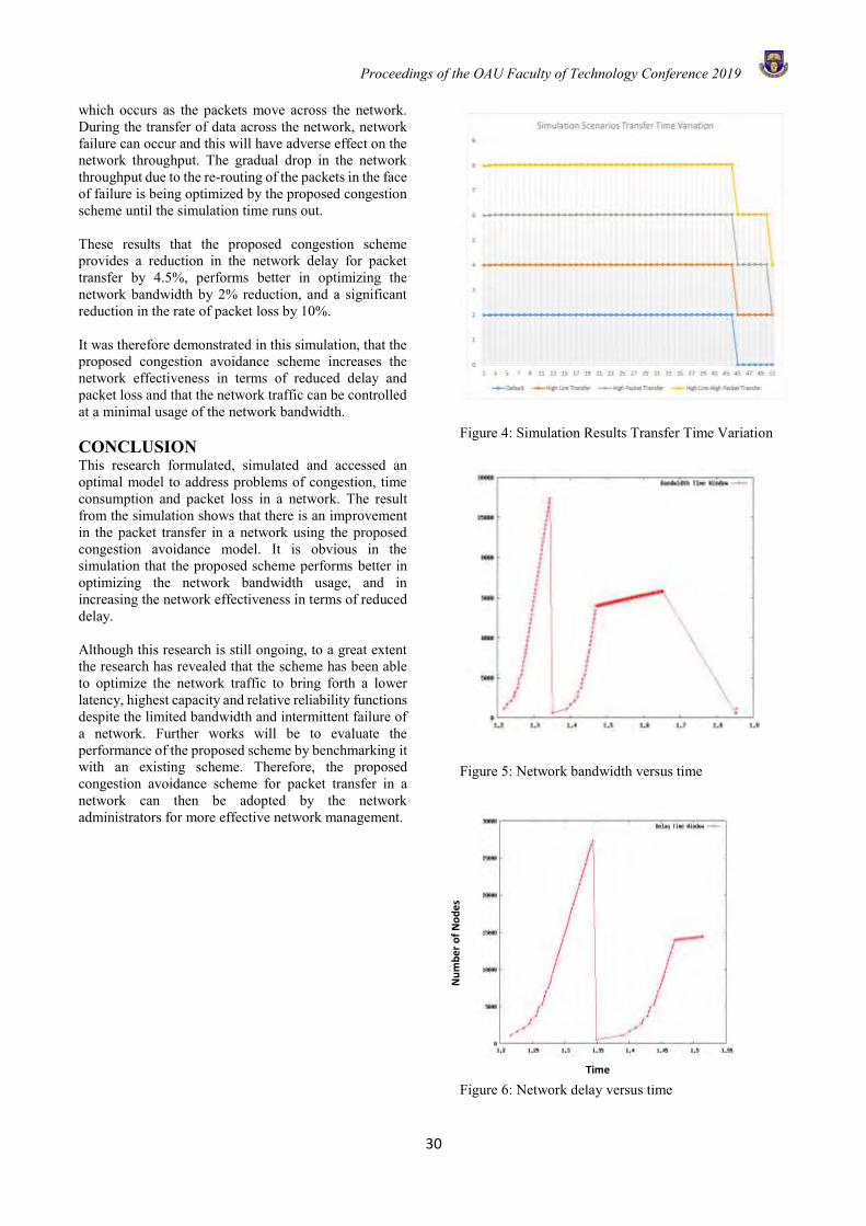
Proceedings of the OAU Faculty of Technology Conference 2019
30
which occurs as the packets move across the network. During the transfer of data across the network, network failure can occur and this will have adverse effect on the network throughput. The gradual drop in the network throughput due to the re-routing of the packets in the face of failure is being optimized by the proposed congestion scheme until the simulation time runs out. These results that the proposed congestion scheme provides a reduction in the network delay for packet transfer by 4.5%, performs better in optimizing the network bandwidth by 2% reduction, and a significant reduction in the rate of packet loss by 10%. It was therefore demonstrated in this simulation, that the proposed congestion avoidance scheme increases the network effectiveness in terms of reduced delay and packet loss and that the network traffic can be controlled at a minimal usage of the network bandwidth. CONCLUSION This research formulated, simulated and accessed an optimal model to address problems of congestion, time consumption and packet loss in a network. The result from the simulation shows that there is an improvement in the packet transfer in a network using the proposed congestion avoidance model. It is obvious in the simulation that the proposed scheme performs better in optimizing the network bandwidth usage, and in increasing the network effectiveness in terms of reduced delay. Although this research is still ongoing, to a great extent the research has revealed that the scheme has been able to optimize the network traffic to bring forth a lower latency, highest capacity and relative reliability functions despite the limited bandwidth and intermittent failure of a network. Further works will be to evaluate the performance of the proposed scheme by benchmarking it with an existing scheme. Therefore, the proposed congestion avoidance scheme for packet transfer in a network can then be adopted by the network administrators for more effective network management.
Figure 4: Simulation Results Transfer Time Variation Figure 5: Network bandwidth versus time
Figure 6: Network delay versus time
Time
(seconds)
Nu
mb
er
of
No
de
s
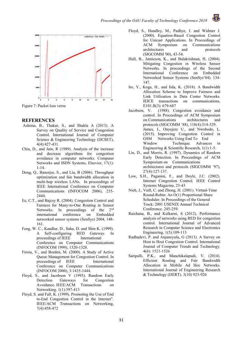
Proceedings of the OAU Faculty of Technology Conference 2019
31
Figure 7: Packet loss versus time REFERENCES Ashima, B., Thakur, S., and Shukla A (2013). A Survey on Quality of Service and Congestion Control. International Journal of Computer Science & Engineering Technology (IJCSET), 4(4):427-431. Chiu, D., and Jain, R (1989). Analysis of the increase and decrease algorithms for congestion avoidance in computer networks. Computer Networks and ISDN Systems, Elsevier, 17(1): 1-14. Dong, Q., Banerjee, S., and Liu, B (2006). Throughput optimization and fair bandwidth allocation in multi-hop wireless LANs. In proceedings of IEEE International Conference on Computer Communications (INFOCOM 2006), 235- 2444. Ee, C.T., and Bajcsy R. (2004). Congestion Control and Fairness for Many-to-One Routing in Sensor Networks. In proceedings of the 2nd international conference on Embedded networked sensor systems (SenSys) 2004, 148- 161. Feng, W. C., Kandlur, D., Saha, D. and Shin K. (1999). A Self-configuring RED Gateway. In proceedings of IEEE International Conference on Computer Communications (INFOCOM 1999), 1320-1328. Firoiu, V., and Borden, M. (2000). A Study of Active Queue Management for Congestion Control. In proceedings of IEEE International Conference on Computer Communications (INFOCOM 2000), 3:1435-1444. Floyd, S., and Jacobson V (1993). Random Early Detection Gateways for Congestion Avoidance. IEEE/ACM Transactions on Networking. 1(1):397-413 Floyd, S. and Fall, K. (1999). Promoting the Use of End to-End Congestion Control in the Internet”. IEEE/ACM Transactions on Networking, 7(4):458-472
Floyd, S., Handley, M., Padhye, J. and Widmer J. (2000). Equation-Based Congestion Control for Unicast Applications. In Proceedings of ACM Symposium on Communications architectures and protocols (SIGCOMM '00), 43-54. Hull, B., Jamieson, K., and Balakrishnan, H. (2004). Mitigating Congestion in Wireless Sensor Networks. In proceedings of the Second International Conference on Embedded Networked Sensor Systems (SenSys’04). 134- 147. Ito, Y., Koga, H., and Iida, K. (2018). A Bandwidth Allocation Scheme to Improve Fairness and Link Utilization in Data Center Networks. IEICE transactions on communications, E101.B(3): 679-687 Jacobson, V. (1988). Congestion avoidance and control. In Proceedings of ACM Symposium on Communications architectures and protocols (SIGCOMM ’88), 118(4):314-329.
James, I., Onyejere U., and Nwobodo, L. (2015). Improving Congestion Control in GSM Networks Using End To End Window Technique. Advances in Engineering & Scientific Research, 1(1):1-5.
Lin, D., and Morris, R. (1997). Dynamics of Random Early Detection. In Proceedings of ACM Symposium on Communications architectures and protocols (SIGCOMM ’97), 27(4):127-137. Low, S.H., Paganini, F., and Doyle, J.C. (2002). Internet Congestion Control. IEEE Control Systems Magazine, 23-43 Nieh, J., Vaill, C. and Zhong, H. (2001). Virtual-Time Round-Robin: An O(1) Proportional Share Scheduler. In Proceedings of the General Track: 2001 USENIX Annual Technical Conference. 245-259. Raichana, B., and Kulkarni, S (2012). Performance analysis of networks using RED for congestion control. International Journal of Advanced Research in Computer Science and Electronics Engineering, 1(5):109-113 Radhadevi, P. and Anjaneyulu, G (2013). A Survey on Host to Host Congestion Control. International Journal of Computer Trends and Technology. 4(6): 1521-1526 Saripalli, P.K., and Manchikalapudi, V. (2014). Efficient Routing and Fair Bandwidth Allocation in Mobile Ad Hoc Networks. International Journal of Engineering Research & Technology (IJERT). 3(10) 923-926
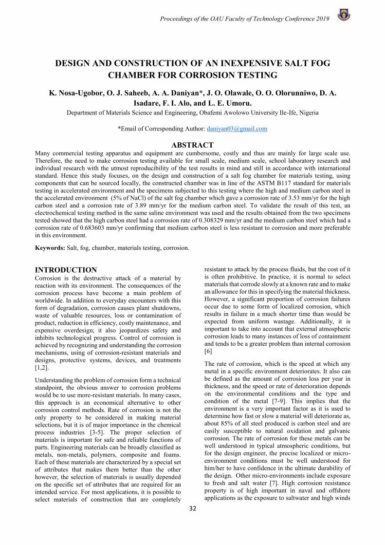
Proceedings of the OAU Faculty of Technology Conference 2019
32
DESIGN AND CONSTRUCTION OF AN INEXPENSIVE SALT FOG CHAMBER FOR CORROSION TESTING
K. Nosa-Ugobor, O. J. Saheeb, A. A. Daniyan*, J. O. Olawale, O. O. Olorunniwo, D. A. Isadare, F. I. Alo, and L. E. Umoru.
Department of Materials Science and Engineering, Obafemi Awolowo University Ile-Ife, Nigeria
*Email of Corresponding Author: [email protected]
ABSTRACT Many commercial testing apparatus and equipment are cumbersome, costly and thus are mainly for large scale use. Therefore, the need to make corrosion testing available for small scale, medium scale, school laboratory research and individual research with the utmost reproducibility of the test results in mind and still in accordance with international standard. Hence this study focuses, on the design and construction of a salt fog chamber for materials testing, using components that can be sourced locally, the constructed chamber was in line of the ASTM B117 standard for materials testing in accelerated environment and the specimens subjected to this testing where the high and medium carbon steel in the accelerated environment (5% of NaCl) of the salt fog chamber which gave a corrosion rate of 3.53 mm/yr for the high carbon steel and a corrosion rate of 3.89 mm/yr for the medium carbon steel. To validate the result of this test, an electrochemical testing method in the same saline environment was used and the results obtained from the two specimens tested showed that the high carbon steel had a corrosion rate of 0.308329 mm/yr and the medium carbon steel which had a corrosion rate of 0.683603 mm/yr confirming that medium carbon steel is less resistant to corrosion and more preferable in this environment.
Keywords: Salt, fog, chamber, materials testing, corrosion.
INTRODUCTION Corrosion is the destructive attack of a material by reaction with its environment. The consequences of the corrosion process have become a main problem of worldwide. In addition to everyday encounters with this form of degradation, corrosion causes plant shutdowns, waste of valuable resources, loss or contamination of product, reduction in efficiency, costly maintenance, and expensive overdesign; it also jeopardizes safety and inhibits technological progress. Control of corrosion is achieved by recognizing and understanding the corrosion mechanisms, using of corrosion-resistant materials and designs, protective systems, devices, and treatments [1,2].
Understanding the problem of corrosion form a technical standpoint, the obvious answer to corrosion problems would be to use more-resistant materials. In many cases, this approach is an economical alternative to other corrosion control methods. Rate of corrosion is not the only property to be considered in making material selections, but it is of major importance in the chemical process industries [3-5]. The proper selection of materials is important for safe and reliable functions of parts. Engineering materials can be broadly classified as metals, non-metals, polymers, composite and foams. Each of these materials are characterized by a special set of attributes that makes them better than the other however, the selection of materials is usually depended on the specific set of attributes that are required for an intended service. For most applications, it is possible to select materials of construction that are completely
resistant to attack by the process fluids, but the cost of it is often prohibitive. In practice, it is normal to select materials that corrode slowly at a known rate and to make an allowance for this in specifying the material thickness. However, a significant proportion of corrosion failures occur due to some form of localized corrosion, which results in failure in a much shorter time than would be expected from uniform wastage. Additionally, it is important to take into account that external atmospheric corrosion leads to many instances of loss of containment and tends to be a greater problem than internal corrosion [6]
The rate of corrosion, which is the speed at which any metal in a specific environment deteriorates. It also can be defined as the amount of corrosion loss per year in thickness, and the speed or rate of deterioration depends on the environmental conditions and the type and condition of the metal [7-9]. This implies that the environment is a very important factor as it is used to determine how fast or slow a material will deteriorate as, about 85% of all steel produced is carbon steel and are easily susceptible to natural oxidation and galvanic corrosion. The rate of corrosion for these metals can be well understood in typical atmospheric conditions, but for the design engineer, the precise localized or micro-environment conditions must be well understood for him/her to have confidence in the ultimate durability of the design. Other micro-environments include exposure to fresh and salt water [7]. High corrosion resistance property is of high important in naval and offshore applications as the exposure to saltwater and high winds
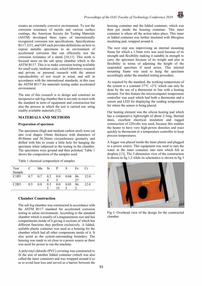
Proceedings of the OAU Faculty of Technology Conference 2019
33
creates an extremely corrosive environment. To test the corrosion resistance of metals and various surface coatings, the American Society for Testing Materials (ASTM) developed three types of internationally recognized corrosion test specifications. Specifications B117, G31, and G85 each provides definitions on how to expose metallic specimens to an environment of accelerated corrosion that can efficiently test the corrosion resistance of a metal [10,11]. This work is focused more on the salt spray chamber which is the ASTM B117. This is to make corrosion testing available for small scale, medium scale, school laboratory research and private or personal research with the utmost reproducibility of test result in mind, and still in accordance with the international standards, in this case the ASTM B117 for materials testing under accelerated environment.
The aim of this research is to design and construct an inexpensive salt fog chamber that is not only to meet with the standard in term of equipment and construction but also the process in which the test is carried out, using readily available materials [12].
MATERIALS AND METHODS
Preparation of specimen
The specimens (high and medium carbon steel) were cut into oval shapes 10mm thickness with diameters of 49.86mm and 50.26mm circumference geometry and drilled with bits to create a little hole for hanging the specimen when subjected to the testing in the chamber. The specimens were ground and then polished. Table 1 shows the composition of the samples used.
Table 1 chemical composition of samples
Test Sample
C Mn Si P S Fe Cr
C1R5 0.7 0.7 0.24
0.05
0.04 86.27
12.0
C2R5 0.5 0.8 0.35
0.035
0.035
86.2
12.0
Chamber Construction
The salt fog chamber was constructed in accordance with the ASTM B117 standard for accelerated corrosion testing in saline environment. According to the standard chamber which is usually of a magnanimous size and has compartments inside of it giving it sections of which has different functions they perform exclusively. A lidded, sealable plastic container was used as a housing for the chamber which had all other components inside of it. It also acted as the system-surrounding boundary. The housing was made to sit close to a power source as there was need for power to run the machine.
A polyvinyl chloride (PVC) covering was constructed to fit the size of another lidded container (which was also called the inner container) and was wrapped around it so as to avoid heat loss and served as a barrier between the
housing container and the lidded container; which was then put inside the housing container. This inner container is where all the action takes place. This inner or lidded container was further insulated with fiberglass insulating pad, wrapped around it.
The next step was improvising an internal mounting frame for which a 1.5mm wire was used because of its strength and flexibility making it suitable in strength to carry the specimen because of its weight and also in flexibility in terms of adjusting the height of the suspended specimen if need arises. This internal mounting frame was used to hang the specimen accordingly under the standard testing procedure.
As required by the standard, the working temperature of the system is a constant 37°C ±2°C which can only be done by the use of a thermostat in line with a heating element. For this feature the microcomputer temperature controller was used which had both a thermostat and a sensor and LED for displaying the reading temperature for where the sensor is being placed.
Our heating element was the silicon heating pad which has a comparative lightweight of about 2-3mg, thermal mass, excellent electrical insulation and rugged construction of 220volts was used, because this enables the heater to have very high-power densities and react quickly to thermostat or a temperature controller to keep process temperatures.
A fogger was placed inside the inner plastic and plugged to a power source. This equipment was used to turn the water in the inner container into mist which fell as droplets [13]. The 3-dimension view of the construction is shown in fig 1,2 while its schematics is shown in fig 3
Fig 1: Overhead view of the design for the constructed chamber
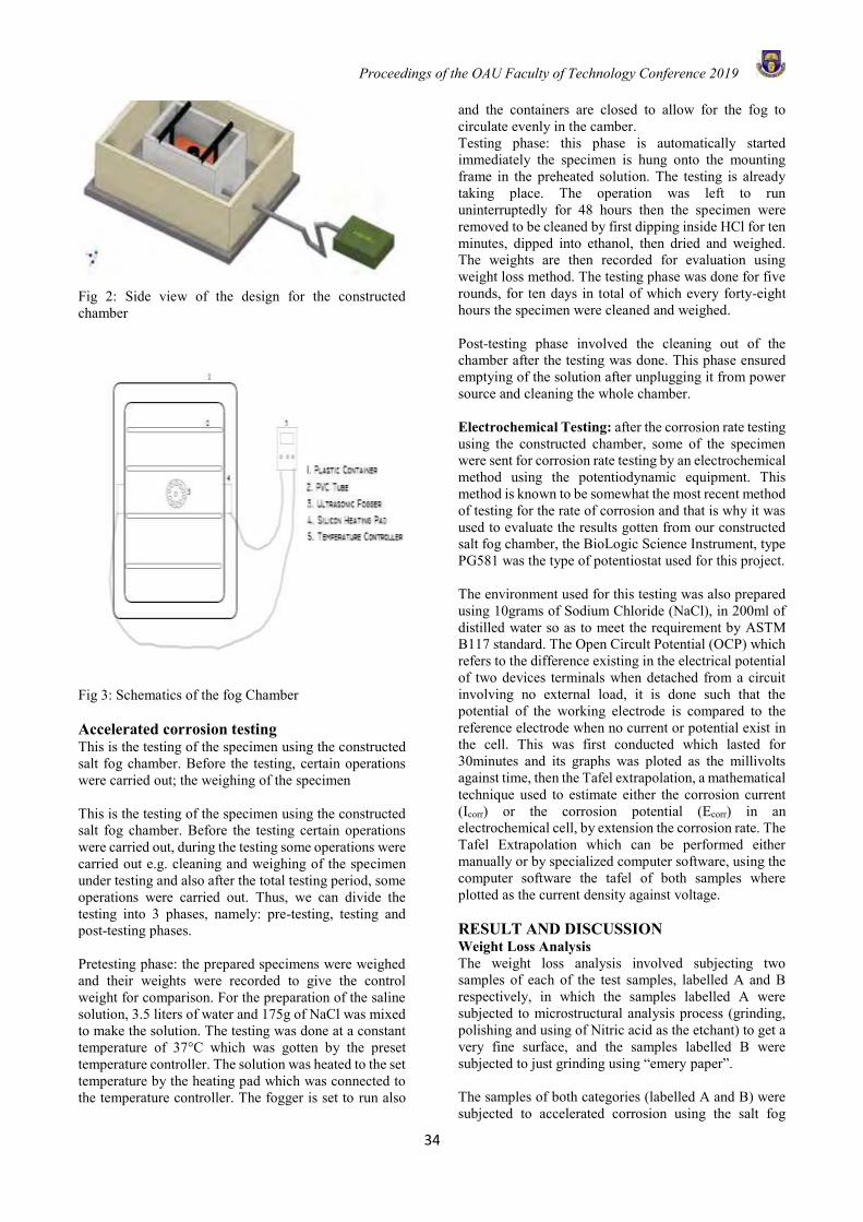
Proceedings of the OAU Faculty of Technology Conference 2019
34
Fig 2: Side view of the design for the constructed chamber
Fig 3: Schematics of the fog Chamber Accelerated corrosion testing This is the testing of the specimen using the constructed salt fog chamber. Before the testing, certain operations were carried out; the weighing of the specimen This is the testing of the specimen using the constructed salt fog chamber. Before the testing certain operations were carried out, during the testing some operations were carried out e.g. cleaning and weighing of the specimen under testing and also after the total testing period, some operations were carried out. Thus, we can divide the testing into 3 phases, namely: pre-testing, testing and post-testing phases. Pretesting phase: the prepared specimens were weighed and their weights were recorded to give the control weight for comparison. For the preparation of the saline solution, 3.5 liters of water and 175g of NaCl was mixed to make the solution. The testing was done at a constant temperature of 37°C which was gotten by the preset temperature controller. The solution was heated to the set temperature by the heating pad which was connected to the temperature controller. The fogger is set to run also
and the containers are closed to allow for the fog to circulate evenly in the camber. Testing phase: this phase is automatically started immediately the specimen is hung onto the mounting frame in the preheated solution. The testing is already taking place. The operation was left to run uninterruptedly for 48 hours then the specimen were removed to be cleaned by first dipping inside HCl for ten minutes, dipped into ethanol, then dried and weighed. The weights are then recorded for evaluation using weight loss method. The testing phase was done for five rounds, for ten days in total of which every forty-eight hours the specimen were cleaned and weighed. Post-testing phase involved the cleaning out of the chamber after the testing was done. This phase ensured emptying of the solution after unplugging it from power source and cleaning the whole chamber. Electrochemical Testing: after the corrosion rate testing using the constructed chamber, some of the specimen were sent for corrosion rate testing by an electrochemical method using the potentiodynamic equipment. This method is known to be somewhat the most recent method of testing for the rate of corrosion and that is why it was used to evaluate the results gotten from our constructed salt fog chamber, the BioLogic Science Instrument, type PG581 was the type of potentiostat used for this project. The environment used for this testing was also prepared using 10grams of Sodium Chloride (NaCl), in 200ml of distilled water so as to meet the requirement by ASTM B117 standard. The Open Circult Potential (OCP) which refers to the difference existing in the electrical potential of two devices terminals when detached from a circuit involving no external load, it is done such that the potential of the working electrode is compared to the reference electrode when no current or potential exist in the cell. This was first conducted which lasted for 30minutes and its graphs was ploted as the millivolts against time, then the Tafel extrapolation, a mathematical technique used to estimate either the corrosion current (Icorr) or the corrosion potential (Ecorr) in an electrochemical cell, by extension the corrosion rate. The Tafel Extrapolation which can be performed either manually or by specialized computer software, using the computer software the tafel of both samples where plotted as the current density against voltage. RESULT AND DISCUSSION Weight Loss Analysis The weight loss analysis involved subjecting two samples of each of the test samples, labelled A and B respectively, in which the samples labelled A were subjected to microstructural analysis process (grinding, polishing and using of Nitric acid as the etchant) to get a very fine surface, and the samples labelled B were subjected to just grinding using “emery paper”. The samples of both categories (labelled A and B) were subjected to accelerated corrosion using the salt fog
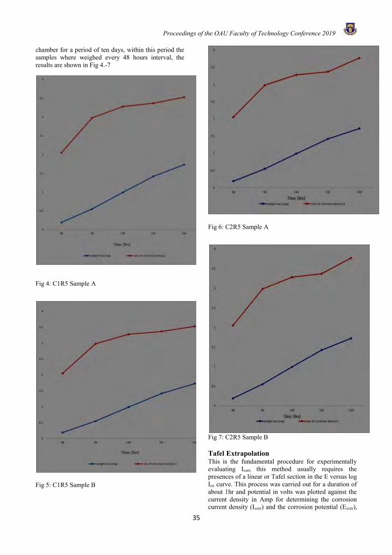
Proceedings of the OAU Faculty of Technology Conference 2019
35
chamber for a period of ten days, within this period the samples where weighed every 48 hours interval, the results are shown in Fig 4.-7
Fig 4: C1R5 Sample A
Fig 5: C1R5 Sample B
Fig 6: C2R5 Sample A
Fig 7: C2R5 Sample B Tafel Extrapolation This is the fundamental procedure for experimentally evaluating Icorr, this method usually requires the presences of a linear or Tafel section in the E versus log Iex curve. This process was carried out for a duration of about 1hr and potential in volts was plotted against the current density in Amp for determining the corrosion current density (Icorr) and the corrosion potential (Ecorr),
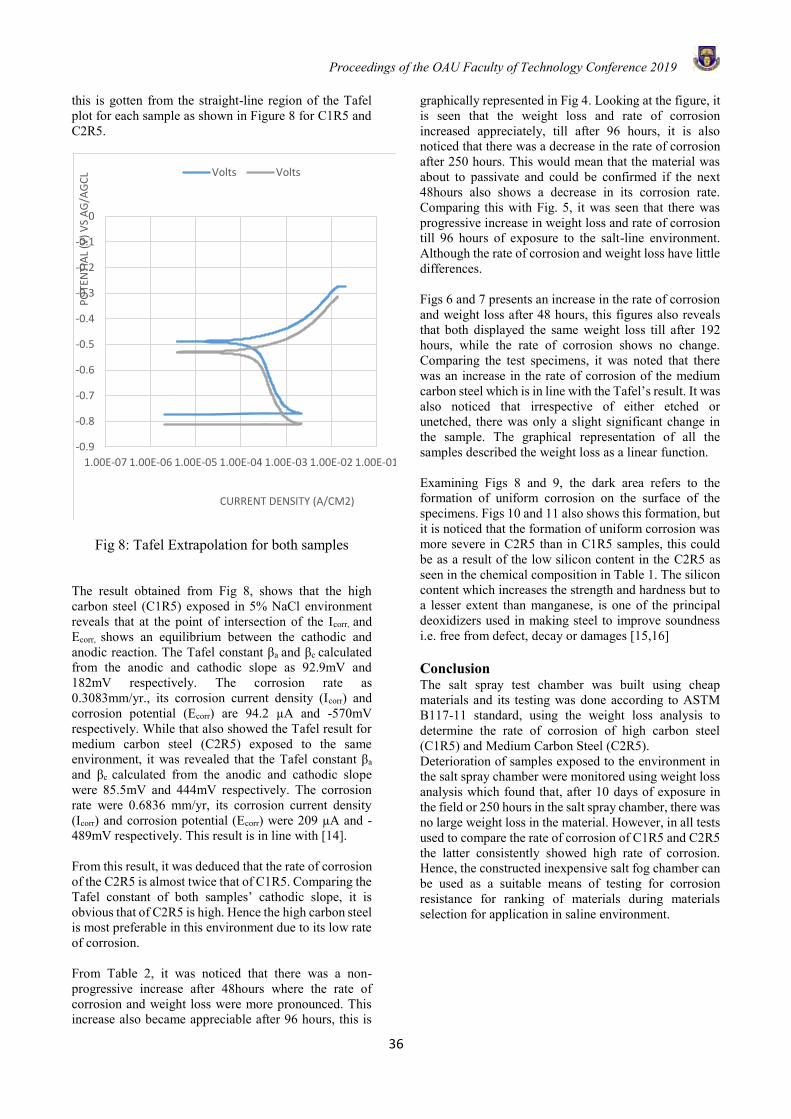
Proceedings of the OAU Faculty of Technology Conference 2019
36
this is gotten from the straight-line region of the Tafel plot for each sample as shown in Figure 8 for C1R5 and C2R5.
Fig 8: Tafel Extrapolation for both samples
The result obtained from Fig 8, shows that the high carbon steel (C1R5) exposed in 5% NaCl environment reveals that at the point of intersection of the Icorr, and Ecorr, shows an equilibrium between the cathodic and anodic reaction. The Tafel constant βa and βc calculated from the anodic and cathodic slope as 92.9mV and 182mV respectively. The corrosion rate as 0.3083mm/yr., its corrosion current density (Icorr) and corrosion potential (Ecorr) are 94.2 µA and -570mV respectively. While that also showed the Tafel result for medium carbon steel (C2R5) exposed to the same environment, it was revealed that the Tafel constant βa and βc calculated from the anodic and cathodic slope were 85.5mV and 444mV respectively. The corrosion rate were 0.6836 mm/yr, its corrosion current density (Icorr) and corrosion potential (Ecorr) were 209 µA and -489mV respectively. This result is in line with [14]. From this result, it was deduced that the rate of corrosion of the C2R5 is almost twice that of C1R5. Comparing the Tafel constant of both samples’ cathodic slope, it is obvious that of C2R5 is high. Hence the high carbon steel is most preferable in this environment due to its low rate of corrosion. From Table 2, it was noticed that there was a non-progressive increase after 48hours where the rate of corrosion and weight loss were more pronounced. This increase also became appreciable after 96 hours, this is
graphically represented in Fig 4. Looking at the figure, it is seen that the weight loss and rate of corrosion increased appreciately, till after 96 hours, it is also noticed that there was a decrease in the rate of corrosion after 250 hours. This would mean that the material was about to passivate and could be confirmed if the next 48hours also shows a decrease in its corrosion rate. Comparing this with Fig. 5, it was seen that there was progressive increase in weight loss and rate of corrosion till 96 hours of exposure to the salt-line environment. Although the rate of corrosion and weight loss have little differences. Figs 6 and 7 presents an increase in the rate of corrosion and weight loss after 48 hours, this figures also reveals that both displayed the same weight loss till after 192 hours, while the rate of corrosion shows no change. Comparing the test specimens, it was noted that there was an increase in the rate of corrosion of the medium carbon steel which is in line with the Tafel’s result. It was also noticed that irrespective of either etched or unetched, there was only a slight significant change in the sample. The graphical representation of all the samples described the weight loss as a linear function. Examining Figs 8 and 9, the dark area refers to the formation of uniform corrosion on the surface of the specimens. Figs 10 and 11 also shows this formation, but it is noticed that the formation of uniform corrosion was more severe in C2R5 than in C1R5 samples, this could be as a result of the low silicon content in the C2R5 as seen in the chemical composition in Table 1. The silicon content which increases the strength and hardness but to a lesser extent than manganese, is one of the principal deoxidizers used in making steel to improve soundness i.e. free from defect, decay or damages [15,16] Conclusion The salt spray test chamber was built using cheap materials and its testing was done according to ASTM B117-11 standard, using the weight loss analysis to determine the rate of corrosion of high carbon steel (C1R5) and Medium Carbon Steel (C2R5). Deterioration of samples exposed to the environment in the salt spray chamber were monitored using weight loss analysis which found that, after 10 days of exposure in the field or 250 hours in the salt spray chamber, there was no large weight loss in the material. However, in all tests used to compare the rate of corrosion of C1R5 and C2R5 the latter consistently showed high rate of corrosion. Hence, the constructed inexpensive salt fog chamber can be used as a suitable means of testing for corrosion resistance for ranking of materials during materials selection for application in saline environment.
-0.9
-0.8
-0.7
-0.6
-0.5
-0.4
-0.3
-0.2
-0.1
0
1.00E-07 1.00E-06 1.00E-05 1.00E-04 1.00E-03 1.00E-02 1.00E-01
PO
TEN
TIA
L (V
) V
S A
G/A
GC
L
CURRENT DENSITY (A/CM2)
Volts Volts

Proceedings of the OAU Faculty of Technology Conference 2019
37
Fig 9: C1R5 Sample A at 600 magnification
Fig 10 : C1R5 Sample B at 600 magnification
Fig 11: C2R5 Sample A at 600 magnification References Roberge, P. R. (2000). Handbook of Corrosion
Engineering. In Introduction (p. 1). United State of America: McGraw-Hill.
Oloruniwo, O. E.. (2018). MSE 507. In O. Dr, Corrossion (pp. 3-7). Ile-Ife Henthorne, M. (1971). Materials Selection for
Corrosion Control, Chemical Engineering. 1139-1146.
Broomfield, J. P., Five Years Research on Corrosion of Steel in Concrete: A Summary of the Strategic Highway Research Program Structures Research, paper no. 318 (Corrosion 93), 1993. Houston, Tex., NACE International.
Ailor, W. H. (1971). Handbook of Corrosion Testing and Evaluation. New York: John Wiley and Sons
corrosion/selection of materials. (2017, September 8). Retrieved from Health and Safety Executive: http://www.hse.gov.uk/comah/sragtech/techmeasmaterials.htm
corrosion/selection of materials. (2017, September 8). Retrieved from Health and Safety Executive: http://www.hse.gov.uk/comah/sragtech/techmeasmaterials.htm
Corrosion rate. (2007, 10 27). Retrieved from Mechanical Engineering: www. mechanicalengineeringsite.com/corrosion-rate-calculation/
Leon, A. D. (2013). Determination of corrosion rate under various corrosive environment using image analysis. International Journal of Science and Technology.
International Stainless Steel Forum. (2008). The Alt Spray and its use in Ranking Stainless Steel. A technical guide to the salt spray test and its interpretation with stainless steel (pp. 5-6). Cricda.

Proceedings of the OAU Faculty of Technology Conference 2019
38
International, A. (2011). Patent No. ASTM B117-11. ISSF. (2008). The salt test and its uses in the ranking of
srainless steel. International Stainless steel forum, May.
Fluoramics, I. (2016, may). Fluoramics, Inc. Retrieved from salt fog chamber: https://www.fluoramics.com/how-to/how-to-construct-an-inexpensive-salt-fog-chamber/Pbcgov. (2016, June 14). UF roof,faster and finals. Retrieved from pbcgov.org: http://discover.pbcgov.org/pzb/building/BCAB/UF-Roof-Fastener-Final-PPT-2016-06-14.pdf
leonghuat. (2007, febuary 09). Element. Retrieved from Leonghuat: leonghuat.com/articles/elements.htm
Lipson, C. and Sheth, N. J. (1973). Statistical Design and Analysis of Engineering Experiments. New York: McGraw-Hill
Proceedings of the OAU Faculty of Technology Conference 2019
39
DESIGN AND IMPLEMENTATION OF A NONLINEAR MODEL PREDICTIVE CONTROLLER ON A NON-MINIMUM PHASE QUADRUPLE
TANK SYSTEM
A.S. Osunleke*, A. Bamimore, I. A. Oyehan, O. O. Ajani and O.A. Olabiyi Department of Chemical Engineering, Obafemi Awolowo University, Ile-Ife, Nigeria.
*Email of Corresponding Author: [email protected]
ABSTRACT Nonlinearity and non-minimum phase, among other features, contribute to retardation in performance of control systems. This phenomenon when not properly attended to makes process systems very challenging to control. Routinely, control engineers employ linear model controller design approach because it is computationally less demanding; although, it gives less satisfactory performance when used on nonlinear systems with or without non-minimum phase feature. To obtain improved system performance, nonlinear controller design approach is preferably implemented. In this article, we designed and implemented nonlinear model predictive controller (NMPC) technique on a locally-built quadruple tank system (QTS) system. Use of QTS is very common in the study of inverse response phenomenon, nonlinearity and multiple input and multiple output (MIMO) control design leading to optimal control problem. For comparative analysis, two controller algorithms - nonlinear model predictive controller and linear model predictive controller (LMPC) were considered in the analysis and design of control mechanism for the quadruple water level system in a non-minimum phase condition via MATLAB simulation package environment. The simulated results were analysed and the controllers’ performances were considered based on faster set point responses, less oscillation, settling time, overshoot and smaller integral absolute error (IAE) and integral square error (ISE) under various operational conditions. The results showed the advantage of NMPC for dealing with the system dynamic over LMPC and could be designed for more complex and fast system dynamics even in the presence of constraints. Keywords: Quadruple tank system, Non-minimum phase, Nonlinear Model Predictive control, Optimal control problem, MIMO. INTRODUCTION Generally, control problem is formulated such that a current state of a controlled system tracks a desired state trajectory as best as possible, in the presence of unknown disturbances and desired state trajectory changes. That is, if the current state is far away from a reference trajectory, appropriate control action is taken to steer the state towards the reference trajectory. If the current state is already close enough to the reference trajectory, appropriate control action is taken to regulate the state there, in the presence of disturbances (Van Der Merwe, 2004), thereby making the control problem easy to solve. However, many times, due to nonlinearity and coupling effects, control problem can be difficult to solve. In this work, a four-tank water level system is presented to demonstrate the effect of input-output interactions, nonlinearity as well as non-minimum phase characteristic. The system considered is a multivariable system with two-input two-outputs. This designed prototypesystem represents a number of MIMO control applications in industry such as paper production processes, chemical processes, metallurgy and biotechnological areas, medical industries, etc. Thus, it could be difficult if not impracticable for conventional PID controller design schemes to handle such systems when subjected to stringent constraints (Fleming and Purhouse, 2001). There available several control techniques for handling system with multiple
interactions, such as: generalised predictive control (Clarke, 1988; Kutnetsov and Clarke, 1994) or any of its extension methods (Osunleke et.al., 2009; Osunleke et.al., 2011; Osunleke et.al., 2016), Model predictive control (Camacho and Burdons, 2004; Mahmoodi et al., 2009) among others. Over the past two decades, Model Predictive Control (MPC) has been proposed as an effective advanced control strategy in process industries. An advantage that it has over PID is its ability to handle system constraints and multivariable interactions naturally within its framework (Koetje, 2010; Alaniz, 2004; Grune and Pannek, 2011). Given process measurements, MPC works by solving a given optimal control problem in real-time to determine the open-loop control variable trajectories and state estimates (Jacob and Dhib, 2011; Qin and Badgwell, 2003). Linear MPC (LMPC) schemes have a long history of being among the most effective advanced control schemes in process industries. Despite their long history of success, LMPC schemes are not considered the best candidates for feedback control of systems that are highly nonlinear. To control such systems adequately without changing the basic MPC principle, researchers and designers in academia and industrial communities derived a direct extension of LMPC called Nonlinear Model Predictive Control (NMPC). A formulation of NMPC problem is similar to that of LMPC problem and owing to that, NMPC has inherited most of the essential
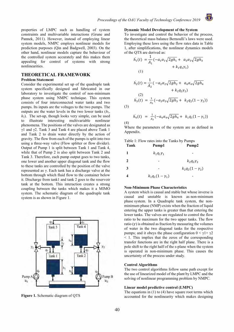
Proceedings of the OAU Faculty of Technology Conference 2019
40
properties of LMPC such as handling of system constraints and multivariable interactions (Grune and Pannek, 2011). However, instead of employing linear system models, NMPC employs nonlinear models for prediction purposes (Qin and Badgwell, 2003). On the other hand, nonlinear models capture the behaviour of the controlled system accurately and this makes them appealing for control of systems with strong nonlinearities. THEORETICAL FRAMEWORK Problem Statement Consider the experimental set up of the quadruple tank system specifically designed and fabricated in our laboratory to investigate the control of non-minimum phase system using NMPC technique. This system consists of four interconnected water tanks and two pumps. Its inputs are the voltages to the two pumps. The outputs are the water levels in the two lower tanks (h1, h2). The set-up, though looks very simple, can be used to illustrate interesting multivariable nonlinear phenomena. The positions of the valves are designated as γ1 and γ2. Tank 3 and Tank 4 are placed above Tank 1 and Tank 2 to drain water directly by the action of gravity. The flow from each of the pumps is split into two using a three-way valve (Flow splitter or flow divider). Output of Pump 1 is split between Tank 1 and Tank 4, while that of Pump 2 is also split between Tank 2 and Tank 3. Therefore, each pump output goes to two tanks, one lower and another upper diagonal tank and the flow to these tanks are controlled by the position of the valve represented as γ. Each tank has a discharge valve at the bottom through which fluid flow to the container below it. Discharge from tank1 and tank 2 goes to the reservoir tank at the bottom. This interaction creates a strong coupling between the tanks which makes it a MIMO system. The schematic diagram of the quadruple tank system is as shown in Figure 1.
Figure 1. Schematic diagram of QTS
Dynamic Model Development of the System To investigate and control the behavior of the process, the theoretical mass balance Bernoulli’s laws were used. Employing these laws using the flow rates data in Table 1, after simplifications, the nonlinear dynamics models of the QTS are derived as:
ℎ1(𝑡) =1
𝐴1
(−𝑎1𝛼1√2𝑔ℎ1 + 𝑎3𝛼3√2𝑔ℎ3
+ 𝑘1𝑞1𝛾1) (1)
ℎ2(𝑡) =1
𝐴2
( −𝑎2𝛼2√2𝑔ℎ2 + 𝑎4𝛼4√2𝑔ℎ4
+ 𝑘2𝑞2𝛾2) (2) ℎ3(𝑡) =
1
𝐴3(−𝑎3𝛼3√2𝑔ℎ3 + 𝑘2𝑞2(1 − 𝛾2))
(3) ℎ4(𝑡) =
1
𝐴3(−𝑎4𝛼4√2𝑔ℎ4 + 𝑘1𝑞1(1 − 𝛾1))
(4) Where the parameters of the system are as defined in Appendix. Table 1: Flow rates into the Tanks by Pumps
Tank Pump1 Pump2
1 𝑘1𝑞1𝛾1 -
2 - 𝑘2𝑞2𝛾2
3 - 𝑘2𝑞2(1 − 𝛾2)
4 𝑘1𝑞1(1 − 𝛾1) -
Non-Minimum Phase Characteristics A system which is causal and stable but whose inverse is causal and unstable is known as non-minimum phase system. In a Quadruple tank system, the non-minimum phase (NMP) exists when the fraction of liquid entering the upper tanks is greater than that entering the lower tanks. The valves are regulated to control the flow ratio to be maximum for the two upper tanks. The flow ratio (𝛾) is obtained as fraction by measuring the volumes of water in the two diagonal tanks for the respective pumps; and it obeys the phase configuration 0 < γ1+ γ2 < 1. This implies that the zeros of the corresponding transfer functions are in the right half plane. There is a pole shift to the right half of the s-plane when the system is operated in non-minimum phase. This causes the uncertainty of the process under study. Control Algorithms The two control algorithms follow same path except for the use of linearized model of the plant by LMPC and the solving of nonlinear programming problem by NMPC. Linear model predictive control (LMPC) The equations in (1) to (4) have square root terms which accounted for the nonlinearity which makes designing

Proceedings of the OAU Faculty of Technology Conference 2019
41
controllers more difficult. The linearized state-space model of the system is given as = 𝑨𝒉 + 𝑩𝒒 (5) 𝒚 = 𝑪𝒉 + 𝑫𝒒 (6) Where, the values of matrices A, B, C and D are given in the Appendix. The above state space was used to design LMPC controller with control horizon and prediction horizon (prediction of state performed over a finite future time interval) of 2 and 50 respectively. Constrained NMPC formulation There are two important separated parts of NMPC problem: a formulation of prediction model and a solution of the optimal control problem. The prediction model is formulated by iterating through the nominal model of the controlled system in order to predict the future state trajectory. Using the model equations (1-4), a general form of discrete-time nonlinear nominal state space model is given by 𝑥(𝑘 + 1) = 𝑓( 𝑥(𝑘), 𝑞(𝑘)) (6) 𝑦(𝑘) = 𝑔( 𝑥(𝑘)) (7) State prediction model The future state prediction is achieved by iterating through the state transition equation given by Equation (6). The state prediction model is described as follows 𝑥(𝑘 + 1𝑘) = 𝑓( 𝑥(𝑘𝑘), 𝑞(𝑘𝑘)) (8) 𝑥(𝑘 + 2𝑘) = 𝑓( 𝑥(𝑘 + 1𝑘), 𝑞(𝑘 + 1𝑘))
(9) 𝑥(𝑘 + 3𝑘) = 𝑓( 𝑥(𝑘 + 2𝑘), 𝑞(𝑘 + 2𝑘)) (10)
.
.
. 𝑥(𝑘 + 𝑁𝑐𝑘) = 𝑓( 𝑥(𝑘 + 𝑁𝑐 − 1𝑘), 𝑞(𝑘 + 𝑁𝑐 −
1𝑘)) (11)
.
.
. 𝑥(𝑘 + 𝑁𝑝𝑘) = 𝑓 ( 𝑥(𝑘 + 𝑁𝑝 − 1𝑘), 𝑞(𝑘 + 𝑁𝑐 −
1𝑘)) (12) where “ 𝑘” means that the state is predicted at time instant k. This pattern is followed until a number of time steps in a prediction horizon, Np is reached. If Nc < Np, the last set of control values 𝑞(𝑘 + 𝑁𝑐 − 1𝑘) in the control sequence is maintained for the remaining (Np - Nc) time steps. Nc is the control horizon. Note that in the formulation of NMPC, Nc is always set to be either less than or equal to Np. This is shown by Equations (8)
through (12). The predicted state trajectory and sequence of control inputs can be put in vector forms as follows
𝑿(𝑘) =
[ 𝑥(𝑘 + 1𝑘)
𝑥(𝑘 + 2𝑘)
𝑥(𝑘 + 3𝑘)⋮
𝑥(𝑘 + 𝑁𝑝𝑘)]
(13)
𝑸(𝑘) =
[
𝑞(𝑘𝑘)
𝑞(𝑘 + 1𝑘)
𝑞(𝑘 + 2𝑘)
𝑞(𝑘 + 3𝑘)⋮
𝑞(𝑘 + 𝑁𝑝 − 1𝑘)]
(14)
Using Equations (13) and (14), Equations (8) through (12) can be summarized as the function of the current state 𝑥(𝑘)= 𝑥(𝑘𝑘) and predicted control input vector 𝑸(𝑘) as follows 𝑿(𝑘 + 1) = 𝑓( 𝑥(𝑘), 𝑸(𝑘)) (15) Output prediction model The predicted state estimates given by Equation (13), but generated from Equation (15) are propagated through the output equation given by Equation (7) in order to determine the predicted output estimates of the system. An output prediction model is described as follows; 𝑦(𝑘 + 1𝑘) = 𝑔( 𝑥(𝑘 + 1𝑘)) (16) 𝑦(𝑘 + 2𝑘) = 𝑔( 𝑥(𝑘 + 2𝑘)) (17) 𝑦(𝑘 + 1𝑘) = 𝑔( 𝑥(𝑘 + 1𝑘)) (18)
⋮ 𝑦(𝑘 + 𝑁𝑝𝑘) = 𝑔 ( 𝑥(𝑘 + 𝑁𝑝𝑘)) (19) The predicted output estimates can be put in a vector form as follows
𝒀(𝑘) =
[ 𝑦(𝑘 + 1𝑘)
𝑦(𝑘 + 2𝑘)
𝑦(𝑘 + 3𝑘)⋮
𝑦(𝑘 + 𝑁𝑝𝑘)]
(20)
Equation (7) can be written in a compact form 𝒀(𝑘) = 𝑔( 𝑥(𝑘)) (21) NMPC algorithm basically solves an optimal control problem to determine an optimal sequence of control inputs such that the controlled system’s future outputs track a given output trajectory which is given by
𝒀𝒔𝒑(𝑘) =
[ 𝑦𝑠𝑝(𝑘 + 1𝑘)
𝑦𝑠𝑝(𝑘 + 2𝑘)
𝑦𝑠𝑝(𝑘 + 3𝑘)⋮
𝑦𝑠𝑝(𝑘 + 𝑁𝑝𝑘)]
(22)
𝒀(𝑘) and 𝑸(𝑘) are the predicted output and control input trajectories that are generated by the NMPC algorithm at every time step k while 𝑌𝑠𝑝(𝑘) is the desired output
Proceedings of the OAU Faculty of Technology Conference 2019
42
trajectory. These are fed into the NMPC algorithm at every time step in order to construct a corresponding cost function which forms part of optimal control problem. Cost function The cost function is quadratic in nature and it is composed of three cost functions𝐽𝑦, 𝐽𝑞 and𝐽𝑑𝑞. The cost function 𝐽𝑦 penalizes a distance of the predicted output trajectory 𝒀(𝑘) from the desired output trajectory 𝒀𝒔𝒑(𝑘) . The quadratic form of 𝐽𝑞 is weighted with positive (semi)-definite weighting matrices (𝑊𝑦(𝑘), … 𝑊𝑦(𝑘 + 𝑁𝑝 − 1)) and hence 𝐽𝑦 is given by 𝐽𝑦 = ∑ (𝑦(𝑘 + 𝑖
𝑁𝑝
𝑖=0𝑘) − 𝑦𝑠𝑝(𝑘 + 𝑖𝑘))𝑇𝑊𝑦(𝑘 + 𝑖) −
(𝑦(𝑘 + 𝑖𝑘) − 𝑦𝑠𝑝(𝑘 + 𝑖𝑘)) (23) When the matrices (𝑊𝑦(𝑘), … 𝑊𝑦(𝑘 + 𝑁𝑝 − 1)) are placed along the main diagonal of an appropriately sized positive (semi) definite weighing matrix 𝑊𝑦(𝑘) as 𝑊𝑦(𝑘) =
[ 𝑊𝑦(𝑘)
0
0 𝑊𝑦(𝑘 + 1)
⋯…
0⋮
⋮ ⋮ ⋱ 0
0 … 0 𝑊𝑦(𝑘+𝑁𝑝 − 1)]
(24)
Cost function 𝐽𝑦 in compact form is 𝐽𝑦 = 𝑌(𝑘) − 𝑌𝑠𝑝(𝑘))𝑇𝑊𝑦(𝑘)(𝑌(𝑘) − 𝑌𝑠𝑝(𝑘)) (25) The cost function 𝐽𝑞 penalizes magnitudes of control inputs in the control sequence 𝑸(𝑘). The quadratic form of the 𝐽𝑞 is weighted with the positive (semi) definite weighing matrices(𝑊𝑞(𝑘), … 𝑊𝑞(𝑘 + 𝑁𝑝 − 1)). 𝐽𝑞 = ∑ 𝑞(𝑘 + 𝑖𝑘)𝑇𝑁𝑝−1
𝑖=0𝑊𝑞(𝑘 + 𝑖) − (𝑞(𝑘 + 𝑖𝑘)
(26) 𝑊𝑞(𝑘) =
[ 𝑊𝑞(𝑘)
0
0 𝑊𝑞(𝑘 + 1)
⋯…
0⋮
⋮ ⋮ ⋱ 0
0 … 0 𝑊𝑞(𝑘+𝑁𝑝 − 1)]
(27)
𝐽𝑞 = 𝑄(𝑘)𝑇𝑊𝑞(𝑘)𝑄(𝑘) (28) The cost function 𝐽𝑑𝑞 penalizes magnitudes of inputs rate. The quadratic form of the 𝐽𝑑𝑞is weighted with the positive (semi) definite weighing matrices(𝑊𝑑𝑞(𝑘), … 𝑊𝑑𝑞(𝑘 + 𝑁𝑝 − 1)). 𝐽𝑑𝑞 = ∑ 𝑑𝑞(𝑘 + 𝑖𝑘)𝑇𝑁𝑝−1
𝑖=0𝑊𝑑𝑞(𝑘 + 𝑖) − (𝑑𝑞(𝑘 +
𝑖𝑘) (29) Where 𝑑𝑞𝑖 = 𝑞𝑖 − 𝑞𝑖−1 (30) Similarly, 𝐽𝑑𝑞 = 𝑑𝑄(𝑘)𝑇𝑊𝑑𝑞(𝑘)𝑑𝑄(𝑘) (31) The total cost function is 𝐽 = 𝐽𝑦 + 𝐽𝑞 + 𝐽𝑑𝑞 (32) Optimal Control Problem (OCP) A process of optimizing a performance of the controlled system corresponds to minimizing J with respect U(k) subjected to equality and inequality constraints of the system. A possible minimum value that J can attain is
zero. This minimization problem is what is technically called an optimal control problem (OCP) for MPC. The OCP can be formulated either as an unconstrained or constrained OCP, depending on whether the constrained satisfaction is desired or not. For the purpose of this work, the constrained OCP is used for the formulation of the constrained NMPC controller. The feature which makes NMPC schemes more attractive for the control of nonlinear dynamic systems is their abilities to handle system constraints in their formulations. In the presence of constraints, the OCP problem is presented as, min 𝑈(𝑥) 𝑌(𝑘) − 𝑌𝑠𝑝(𝑘))𝑇𝑊𝑦(𝑘)(𝑌(𝑘) − 𝑌𝑠𝑝(𝑘)) +
𝑄(𝑘)𝑇𝑊𝑞(𝑘)𝑄(𝑘) + (𝑘)𝑇𝑊𝑑𝑞(𝑘)𝑑𝑄(𝑘) (33) Subject to,
𝑥(𝑘 + 𝑖𝑘) = 𝑓( 𝑥(𝑘 + 𝑖 − 1𝑘),
𝑞(𝑘 + 𝑖 − 1𝑘)) (34)
𝑦(𝑘 + 𝑖𝑘) = 𝑔( 𝑥(𝑘 + 𝑖 − 1𝑘)), 𝑖 = 0,… , 𝑁𝑝 − 1 (35) 𝑞(𝑘 + 𝑖𝑘) = 𝑞(𝑘 + 𝑁𝑐 − 1𝑘), 𝑖 = 𝑁𝑐 , … , 𝑁𝑝 − 1 (36) 𝑋𝑚𝑖𝑛 ≤ 𝑋(𝑘) ≤ 𝑋𝑚𝑎𝑥 (37) 𝑄𝑚𝑖𝑛 ≤ 𝑄(𝑘) ≤ 𝑄𝑚𝑎𝑥 (38) 𝑌𝑚𝑖𝑛 ≤ 𝑌(𝑘) ≤ 𝑌𝑚𝑎𝑥 (39) 𝑑𝑄𝑚𝑖𝑛 ≤ 𝑑𝑄(𝑘) ≤ 𝑑𝑄𝑚𝑎𝑥 (40) where 𝑋𝑚𝑖𝑛,𝑌𝑚𝑖𝑛 , 𝑄𝑚𝑖𝑛 and 𝑑𝑄𝑚𝑖𝑛 are the lower bounds of the state trajectory, system output trajectory, sequence of control inputs and input rate respectively.𝑋𝑚𝑎𝑥 ,𝑌𝑚𝑎𝑥 , 𝑄𝑚𝑎𝑥 and 𝑑𝑄𝑚𝑎𝑥 are the upper bounds of the state trajectory, system output trajectory, sequence of control inputs and input rate respectively. Equations (37) through (40) describe the inequality constraints of the system. Equality constraints are described by the equation (34) to (36). Discretization of OCP This is a process of transforming OCP into a standard nonlinear programming (NLP) so as to solve the OCP using solution methods such as sequential quadratic programming (SQP). A standard NLP is described as min 𝐹(𝑧(𝑘)) subject to: 𝐻(𝑧(𝑘)) = 0 (41) 𝐺(𝑧(𝑘)) ≤ 0 (42) Where F is the cost function of the problem and 𝑧(𝑘) is the optimization variable. SIMULATION RESULTS One of the advantages of NMPC algorithms is the high degree of configuration that they offer (control and prediction horizons, penalization terms, etc.). The
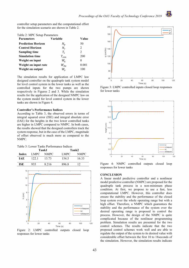
Proceedings of the OAU Faculty of Technology Conference 2019
43
controller setup parameters and the computational effort for the simulation scenario are shown in Table 2. Table 2: MPC Setup Parameters
Parameters Variable Value Prediction Horizon 𝑁𝑝 50 Control Horizon 𝑁𝑐 2 Sampling time 𝑇𝑠 2 Simulation time 𝑇𝑠𝑖𝑚 200 Weight on input 𝑊𝑞 0 Weight on input rate 𝑊𝑑𝑞 0.001 Weight on output 𝑊𝑦 100
The simulation results for application of LMPC law designed controller on the quadruple tank system model for level control system in the lower tanks as well as the controlled inputs for the two pumps are shown respectively in Figures 2 and 3. While the simulation results for the application of the designed NMPC law on the system model for level control system in the lower tanks are shown in Figure 4. Controller’s Performance Indices According to Table 3, the observed errors in terms of integral squared error (ISE) and integral absolute error (IAE) for the heights in the two lower controlled tanks are higher in LMPC compared to NMPC. In both cases, the results showed that the designed controllers track the system response, but in the case of the LMPC, magnitude of offset observed is much more as compared to the NMPC. Table 3: Lower Tanks Performance Indices
Tank1 Tank2 Index LMPC NMPC LMPC NMPC IAE 122.1 13.73 154.5 16.33
ISE 935 8.216 896.8 12
Figure 2: LMPC controlled outputs closed loop responses for lower tanks
Figure 3: LMPC controlled inputs closed loop responses for lower tanks
Figure 4: NMPC controlled outputs closed loop responses for lower tanks CONCLUSION A linear model predictive controller and a nonlinear model predictive controller (NMPC) are proposed for the quadruple tank process in a non-minimum phase condition. At first, we propose to use a fast, less computational LMPC. However, this controller does ensure the stability and the performance of the closed loop system over the whole operating range but with a high offset. Therefore, a NMPC which guarantees the stability and the performance of the system over the desired operating range is proposed to control the process. However, the design of the NMPC is quite complicated because of the nonlinear programming problem. Simulation results are presented for the two control schemes. The results indicate that the two proposed control schemes work well and are able to regulate the output of the system to its desired value with considerable offset between the first 10 to 18seconds of the simulation. However, the simulation results indicate
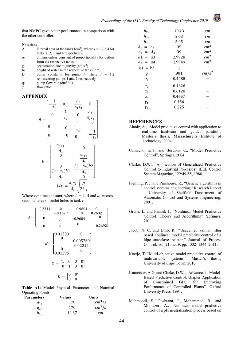
Proceedings of the OAU Faculty of Technology Conference 2019
44
that NMPC gave better performance in comparison with the other controller. Notations Ai internal area of the tanks (cm2), where i = 1,2,3,4 for
tanks 1, 2, 3 and 4 respectively. αi dimensionless constant of proportionality for outlets
from the respective tanks g acceleration due to gravity (cm s-2) hi height of water in the respective tanks (cm) kj pump constants for pump j, where j = 1,2
representing pumps 1 and 2 respectively qj pump flow rate (cm3 s-1) γ flow ratio APPENDIX
𝐴 =
[ −
1
𝜏1
0
0 −1
𝜏2
𝐴3
𝐴1𝜏3
0
0𝐴4
𝐴2𝜏4
0
0
0 0
−1
𝜏3 0
0
−1
𝜏1]
𝐵 =
[
γ1𝑘1
𝐴1
0
0 0
(1 − γ1)𝑘1
𝐴4
γ2𝑘2
𝐴2
(1 − γ2)𝑘2
𝐴3
0 ]
1/𝜏𝑖 =𝑎𝑖𝛼𝑖
𝐴𝑖√
𝑔
2ℎ𝑖𝑠
Where 𝜏𝑖= time constant, where 𝑖 = 1...4 and 𝑎𝑖 = cross sectional area of outlet holes in tank 𝑖
𝐴 =
[ −0.2311 0
0 −0.16790.9604 0
0 0.2692 0
0
0 0
−0.9604 0
0
−0.2692]
𝐵 =
[ 0.01303 0
0 0
0.01395
0.0057690.02214
0 ]
𝐶 = [
1 0 0 00 1 0 0
]
𝐷 = [0 00 0
] Table A1: Model Physical Parameter and Nominal Operating Points
Parameters Values Units 𝑞10
170 𝑐𝑚3/𝑠 𝑞20
170 𝑐𝑚3/𝑠 ℎ10
12.37 𝑐𝑚
ℎ20 10.23 𝑐𝑚
ℎ30 2.63 𝑐𝑚
ℎ40 5.05 𝑐𝑚
𝐴1 = 𝐴3 35 𝑐𝑚2 𝐴2 = 𝐴4 39 𝑐𝑚2 𝑎1 = 𝑎3 2.9928 𝑐𝑚2 𝑎2 = 𝑎4 1.9949 𝑐𝑚2 𝑘1 = 𝑘2 1 −
𝑔 981 𝑐𝑚/𝑠2 𝛼1 0.4488 −
𝛼2 0.4626 − 𝛼3 0.6128 − 𝛼4 0.4657 − 𝛾1 0.456 − 𝛾2 0.225 −
REFERENCES Alaniz, A., “Model predictive control with application to
real-time hardware and guided parafoil”, Master’s thesis, Massachusetts Institute of Technology, 2004.
Camacho, E. F. and Bordons. C., “Model Predictive
Control”, Springer, 2004. Clarke, D.W., “Application of Generalized Predictive
Control to Industrial Processes” IEEE Control System Magazine, 122:49-55, 1988.
Fleming, P. J. and Purshouse, R., “Genetic algorithms in
control systems engineering,” Research Report - University of Sheffield Department of Automatic Control and Systems Engineering, 2001.
Grune, L. and Pannek J., “Nonlinear Model Predictive
Control: Theory and Algorithms”. Springer, 2011.
Jacob, N. C. and Dhib, R., “Unscented kalman filter
based nonlinear model predictive control of a ldpe autoclave reactor,” Journal of Process Control, vol. 21, no. 9, pp. 1332–1344, 2011.
Koetje, T. “Multi-objective model predictive control of
multivariable systems,” Master’s thesis, University of Cape Town, 2010.
Kutnetsov, A.G. and Clarke, D.W., “Advances in Model-
Based Predictive Control, chapter Application of Constrained GPC for Improving Performance of Controlled Plants”. Oxford University Press, 1994.
Mahmoodi, S., Poshtana, J., Mohammad, R., and
Montazeri, A., “Nonlinear model predictive control of a pH neutralization process based on

Proceedings of the OAU Faculty of Technology Conference 2019
45
Wiener–Laguerre model’’, in Chemical Engineering Journal, 146:328–337, 2009.
Osunleke, A. S., Deng, M. and Inoue, A- A CAGPC
Controller Design for Systems with Input Windup and Disturbances. International Journal of Innovative Computing, Information and Control, 5(10B):3517-3526, 2009.
Osunleke, A.S., Deng, M. and Akira, Y. “A Design
Procedure for Control of Strictly Proper Non-Minimum Phase Processes with Input Constraints and Disturbance”, International Journal of Modelling, Identification and Control, 13(1/2): 46-55, 2011.
Osunleke, A.S., Bamimore, A., Sogunle, O. and Taiwo,
O., “Analytical Design of CGPC-based PID Controllers for Commonly Encountered Engineering Systems”, LAUTECH Journal of Engineering and Technology, 9(2):28-33, 2015.
Qin, S. J. and Badgwell, T. A., “A survey of industrial
model predictive control technology”, Control engineering practice, vol. 11, no. 7, pp. 733–764, 2003.
Van der Merwe, R., “Sigma−Point Kalman filters for
probabilistic inference in dynamic state−Space models,” Ph.D Thesis, OGI School of Science and Engineering, Oregon Health and Science University, April, 2004.
Proceedings of the OAU Faculty of Technology Conference 2019
46
DESIGN AND IMPLEMENTATION OF GSM-BASED ENERGY THEFT DETECTION IN A SINGLE-PHASE SMART METER
D. T. Sawyer*1 and F. K. Ariyo1 1 Department of Electronic and Electrical Engineering
Obafemi Awolowo University, Ile-Ife, Nigeria
*Email of Corresponding Author: [email protected]
ABSTRACT In this study, a GSM-based Single-phase smart meter was developed with energy theft detection; meter bypassing and tampering, employing current differential principle. These were with a view to effectively curb energy theft in residential buildings, thereby improving and reducing the distributed energy losses in distribution system and to minimise loss of revenue in the power industry. The smart meter unit was designed to measure energy usage, control the connection of the user remotely and also to communicate with the utility and the remote user interface unit. The remote communication between the consumer’s meter and power utility company were established with the aid of Global System for Mobile Communication (GSM) module. The energy theft detection unit was designed using two current sensors connected to both live and neutral wire interfaced respectively to the analogue input pins of an Arduino Nano microcontroller board and was sampled simultaneously. A light dependent resistor (LDR) was connected to the analogue input pin of the Arduino Nano microcontroller board to detect tampering due to opening of meter casing. The results obtained from the study showed good system performance and the energy meter has a capacity of measuring minimum and maximum load current of 2 mA and 40 A respectively. The electrical smart meter was able to detect energy theft effectively and energy loss was significantly reduced and power quality improved. Keywords: Smart meter, Energy theft, Power quality, GSM module, Microcontroller. INTRODUCTION Electricity is widely used in modern society, it increases productivity and enhances the living condition in people’s daily life (Wang and Qi, 2012). In Nigeria, Nigeria Electricity Regulatory Commission (NERC) states that power delivery frequency should be 50 Hz. Electricity is used to operate domestic, commercial and industrial loads. The amount of energy consumed either by households or industries is measured by an electricity energy meter. The meter aids in the generation of accurate bills for the consumer among others Weranga et al. (2014). Over the years, different types of energy measuring meters has evolved, from the electromechnical meter to the smart meter with the purpose of attaining best and efficient solutions for energy conservation etc Živic et al. (2015). Power utility companies in developing and developed countries especially in Nigeria are faced majorly with low billing, tampering and energy theft problems. Smart meter with tamper proof and energy theft detection functionalities will help the power utilities with increased revenues Megalingam et al. (2011). In Nigeria and some other developing countries, energy theft has emerged as one of the leading issues the power utility company is challenged with, as it results in loss of revenue to the electricity companies. As presented by Olaoluwa (2017), energy theft is an offense and this act causes tariff increase and load shedding on the legal consumers, while on the distribution system, load increase and frequency decrease. In Nigeria, energy theft is yet to be a criminal offence which prevents the distribution company from adequately punishing
offenders. When offenders are caught in the act, they are charged to pay for the loss of revenue which is difficult to estimate and usually much lower than the actual cost of energy stolen Adedamola (2018). Under Nigeria’s Criminal Code Act, (2004) which was passed into law in 2005, is the legal framework governing the electricity supply industry in Nigeria, under Part 6: division 1 & 2, which covers property theft and vandalism in various areas and its offences, but did not cover energy theft. Also, Electric Power Sector Reform Act (EPSRA), 2005 neither recognizes energy theft nor mandates any punishment for it. The major forms of energy theft includes meter tampering, meter bypass, unpaid bills, billing irregularities, etc. According to NERC Third Quarter Report, (2018), it was observed that for every ₦10 worth of electricity received by the distribution company, ₦1.90 is lost due to poor distribution infrastructure and energy theft. Also, as presented by the Ikeja Electricity Distribution Company IKEDC (2014), out of the 134,000 prepaid meters installed by the company, at least 43,000 meters have been tampered with by the consumers. In the past, different non-technical and technical methods have been proposed to detect energy theft Megalingam et al. (2011) Investigation of the consumers with suspicious load-profile was the non-technical method adpoted while harmonic generator, extreme learning machine techniques etc.. were the technical methods employed to detect energy theft in distribution systems (Depuru et al., 2010; Dike et al., 2015; Manojkumar et al., 2016). If good communication system is ensured, only then will the various technical
Proceedings of the OAU Faculty of Technology Conference 2019
47
methods be implemented effectively. Among other schemes reviewed for the controlling of energy theft, smart meter emerged the best considering the efficiency, reliability of the system, and economy cost. Thus, it led to the innovation of smart meter which is of great importance to this study (Nabil et al., 2013; Sardar and Ahmad, 2016).
Several works have been conducted in this area of research using different methods in controlling energy theft. This paper presents an effective method, which uses current differential theory to determine energy theft due to bypassing and tampering to improve the power quality and reduce revenue loss in distribution systems. Javali et al (2017) study is similar in terms of method but different in terms of the parameters measured (L1 and L2), the parameters measured in this study: L1 and N2 for energy theft detection. And for tampering, this study used LDR while javali et al used Seal Break Sense Switch for meter cover opening. LITERATURE REVIEW Several works have been conducted in the area of determining, detecting and controlling energy theft. This section of the paper reviews some of the works conducted in this area. A brief survey of various methods, solutions and limitations are presented. In Patil et al. (2013), the system was able to identify theft detection using the mathematical model: difference in power values of the total transmitted energy and the consumed energy through meter readings, a wireless communication medium was used to convey the information and disconnection of the power supply was done locally. This system actually identifies the exact location of tapping done on distribution lines (in theory). The limitation of the work was that the system was expensive and a bit complex; hence the system was not implemented. Depuru et al. (2010) in their work discussed the factors that cause consumers to engage in energy theft, methods for detecting and estimating theft were also examined. This paper proposed a design of smart meter circuit with the aim of detecting electricity theft, conserved and effectively utilized energy. One major benefit of this method was the ability of the system to identify genuine consumers and disconnect them before the harmonic generator was operated. The research was not implemented. The setback however is that harmonics in distribution system contributes to low or deterioration power quality. Smith (2004) carried out an intensive study on electricity theft and its various ways. According to his research, electricity theft could be estimated, but not measured exactly. The most accurate estimate of theft was by conducting a thorough analysis of the power system. The standard method of measuring electricity theft is by the analysis of transmission and distribution losses (T&D losses). A wireless electricity theft detection and monitoring system was designed by Sharma et al. (2016) using AT89S52/C51 microcontroller, relays, opto-couplers, precaution module, among others that detects energy theft on distribution line and report to appropriate quarters of the development as well as
monitoring the power consumption of the consumer via Global System for Mobile Communication (GSM). The upside of the proposed methodology was that it could detect theft as well as the location of the theft and also it could detect short-circuit. The downside of the system was that it will be too expensive to implement. Results from the study show good system performance. Anil et al. (2016) designed a smart meter using Atmega328p microcontroller and Hall effect sensor for current sensing and computing the meter’s energy measurement, which monitors the power and energy consumption of a consumer and identifies theft. The energy meter was interfaced to a wireless transmission for bi-directional communication to the power utility control centre. One major benefit of this method is the meter’s capability to monitor energy and power usage of consumer remotely and in real-time. Anshul et al. (2015), in their work designed a tampering detection energy meter. The limitation of their work was the lack of disconnecting the supply to the load by power utility through SMS in case of tampering.
METHODOLOGY The smart electrical energy metering system was designed to have three functional units which were the smart metering unit, energy theft detection unit and communication unit. The smart metering unit was developed for connecting and disconnecting electricity supply and measuring power consumption. The energy theft detection unit, which has two hall-effect current sensors, and LDR for detecting energy theft based on meter by-pass and tampering and display the information on an LED. The communication unit has a GSM module that communicates with the smart metering unit and was also responsible for the transmission unit of energy theft by the user to the power distribution company. The circuit diagram of the smart meter is presented in Figure 1and the flowchart in figure 2.
Smart Meter Design A microcontroller board was used for computation and control. Also, a voltage and current sensing unit were used to measure the supply voltage and the current drawn from the mains by the consumer’s loads respectively. The voltage sensing unit was connected to analogue pin A0 of the microcontroller while the current sensing unit was connected to analogue pin A2 respectively. The data from these sensors was used to compute power consumption and energy usage. A SIM-800L GSM modem was connected to pins 8 and 9 of the microcontroller to allow serial communication with the GSM module and by extension, the power distribution company. A relay was connected to pin 10 of the microcontroller to connect and disconnect the consumer from the mains in the event of energy theft detection or tampering. The consumer was connected to the mains only when there are no irregularities in the system. In addition, a power supply unit was integrated into the design to power the other parts of the smart metering unit at the required voltages.

Proceedings of the OAU Faculty of Technology Conference 2019
48
Communication Unit Design Similar to the other units, a microcontroller board was also used to perform computation and control of the remote. An LCD was connected to pins D4 – D7, 2, and 3 of the microcontroller. The LCD displays energy and consumed power information, received from the smart meter unit. A SIM800 GSM Module was connected to pins 8 and 9 of the microcontroller to allow serial
communication between the smart meter unit and the power distribution company. Energy Theft Detection Design Two current sensors connected to both live and neutral wire were interfaced respectively to the microcontroller on pins A0 – A2. Current through live cable denoted as iL and the current through Neutral cable denoted as iN are
Figure 1 Circuit Diagram of Smart Meter
sampled simultaneously; if the difference between LI
and NI is greater than 0.20 A as in equation 1 below, then alarm for energy theft is raised; and the highest of the two is used to compute the energy consumed. A tolerance value of 0.20 A was chosen for the difference this is because of the various components such as the transformer, relay and other discrete components used in the smart meter that consumes a particular amount of power.
LI - NI .> 0.20 (1)
where,
LI = current in live cable
NI = current in neutral cable
And the load current was computed as shown in equation 2
21
1 Nrms nn
I IN =
= (2)
where,
I1, I2 … In are the values of the currents measured by the current sensor at the first, second and up till the Nth sample interval.
A LDR was connected to pin A6 of the microcontroller to detect tampering on the meter. A relay was connected to pin D12 of the microcontroller to connect and disconnect the consumer from the mains during the occurrence of energy theft on the smart meter. Furthermore, a power supply unit supplies power to the other parts of the units at the required voltages.
RESULTS AND DISCUSSION The meter by-pass capability was tested by connecting different loads of varying capacity. For the meter-bypass, it was observed that the GSM response time increases as the load increases. This is summarized in Table 2. In the case of tampering, an attempt was made to open the casing of the meter, this expose the LDR to light. The resistance of the LDR decreases and meter tampering was detected. In the case of the above energy theft, an SMS command to disconnect ‘0#’ the user from the supply was sent to the designated SIM number contained in GSM module. It took 5 secs to disconnect the consumer.
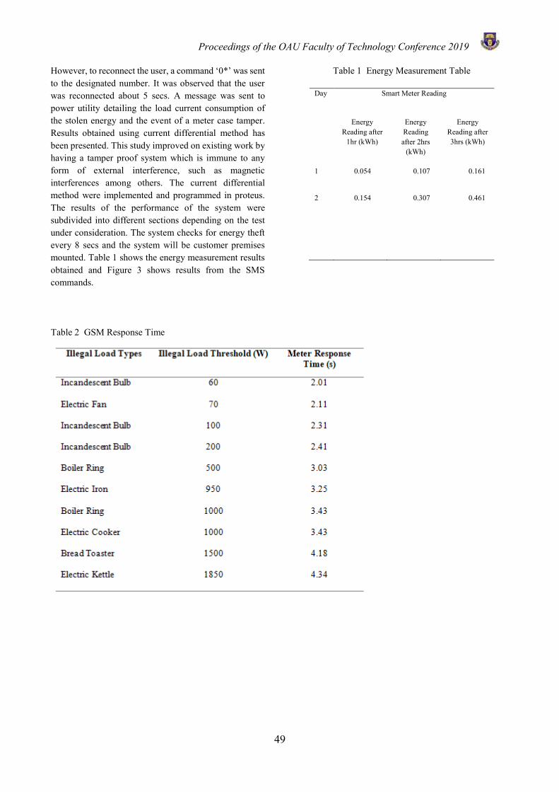
Proceedings of the OAU Faculty of Technology Conference 2019
49
However, to reconnect the user, a command ‘0*’ was sent to the designated number. It was observed that the user was reconnected about 5 secs. A message was sent to power utility detailing the load current consumption of the stolen energy and the event of a meter case tamper. Results obtained using current differential method has been presented. This study improved on existing work by having a tamper proof system which is immune to any form of external interference, such as magnetic interferences among others. The current differential method were implemented and programmed in proteus. The results of the performance of the system were subdivided into different sections depending on the test under consideration. The system checks for energy theft every 8 secs and the system will be customer premises mounted. Table 1 shows the energy measurement results obtained and Figure 3 shows results from the SMS commands.
Table 1 Energy Measurement Table
Day Smart Meter Reading
Energy Reading after
1hr (kWh)
Energy Reading after 2hrs
(kWh)
Energy Reading after 3hrs (kWh)
1
2
0.054
0.154
0.107
0.307
0.161
0.461
Table 2 GSM Response Time
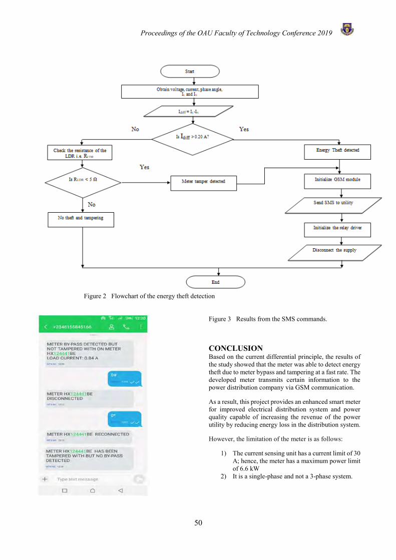
Proceedings of the OAU Faculty of Technology Conference 2019
50
Figure 2 Flowchart of the energy theft detection
Figure 3 Results from the SMS commands.
CONCLUSION Based on the current differential principle, the results of the study showed that the meter was able to detect energy theft due to meter bypass and tampering at a fast rate. The developed meter transmits certain information to the power distribution company via GSM communication.
As a result, this project provides an enhanced smart meter for improved electrical distribution system and power quality capable of increasing the revenue of the power utility by reducing energy loss in the distribution system.
However, the limitation of the meter is as follows:
1) The current sensing unit has a current limit of 30 A; hence, the meter has a maximum power limit of 6.6 kW
2) It is a single-phase and not a 3-phase system.
Proceedings of the OAU Faculty of Technology Conference 2019
51
REFERENCE Adedamola, A., Mitigating Electricity Theft in Nigeria.
1-12, 2018. Anil, K., Prashanth, B., and Saurabh, A., Design and
Implementation of Wireless Energy Meter System for Monitoring the Single Phase Supply. International Journal of Computer Applications, 41(2):26-29, 2016.
Anshul, S., Patel, I., Axat, S., and Anuradha, D., Tampering Detection Of Energy Meter By Gsm Modem. International Journal of Engineering Innovation & Research (IJEIR), 4(3):433-440, 2015.
Criminal Code Act. (2004). Laws of the Federal Republic of Nigeria 2004.
Depuru, S. S. S. R., Wang, L., and Devabhaktuni., V., Electricity theft: Overview, issues, prevention and a smart meter based approach to control theft. Elsevier Ltd, 1007–1015, 2010.
Dike, D. O., Obiora, U. A., Nwokorie, E. C., and Dike, B. C., Minimizing Household Electricity Theft in Nigeria Using GSM Based Prepaid Meter. American Journal of Engineering Research (AJER), 4(1):59-69, 2015.
Electric Power Sector Reform Act (EPSRA), 2005 IKEDC., 43,000 Installed Prepaid Meters Already
Tampered With, 2014. Retrieved November 21, 2018 https://www.nigeriaelectricityhub.com/2014/06/10/43000-installed-prepaid-meters-already-tampered-with-ikedc/
Manojkumar, M. P., Prasanna, R. M., Shakti, L., Sneha, S., and Chandrakant, U., GSM Based Power Theft Detection System Using Android. International Journal of Engineering Science and Computing (IJESC), 6(5):6016-6018, 2016.
Megalingam, R. K., Krishnan, A., Ranjan, B. K., Nair, A. K., Vidyapeetham, A. V., Amritapuri, and Clappana, P. O., Advanced Digital Smart Meter for Dynamic Billing, Tamper Detection and Consumer Awareness. 3rd IEEE International Conference on Electronics Computer Technology, 389-393, 2011.
NERC Third Quarter Report., Nigerian Electricity Regulatory Commission (NERC) Quarterly Report, 2018.
Nigeria Electricity Regulatory Commission (NERC), The Distribution Code For The Nigeria Electricity Distribution System - Version 01, 2016
Olaoluwa, O. G., Electricity Theft and Power Quality in Nigeria. International Journal of Engineering Research & Technology (IJERT), 6(6):1180-1184, 2017.
Patil, S., Pawaskar, G., and Patil, K., Electrical Power Theft Detection and Wireless Meter Reading. International Journal of Innovative Research in
Science, Engineering and Technology, 2(4):1114-1119, 2013.
Sardar, S., and Ahmad, S., Detecting And Minimizing Electricity Theft: A Review, 2016
Sharma, P., Gupta, H., Sharma, M., Singh, R., and Khan, A., Wireless Electricity Theft Detection And Monitoring. International Journal of Advanced Research in Electronics and Communication Engineering (IJARECE), 5(4):994-998, 2016.
Smith, T. B., Electricity theft: a comparative analysis. Energy Policy, 32(18):2067–2076, 2004.
Wang, J., and Qi, C., The Design of Control System for Smart Meter. IEEE Computer Society, 1961-1964, 2012.
Weranga, K. S. K., Kumarawadu, S., and Chandima, D. P., Smart Metering Design and Applications. Singapore: Springer Publishers, 2014.
Živic, N. S., Ur-Rehman, O., and Ruland, C., Evolution of Smart Metering Systems. 23rd IEEE Telecommunications forum (TELFOR), 635-638, 2015.

Proceedings of the OAU Faculty of Technology Conference 2019
52
DEVELOPMENT OF A LOW-COST PROGRAMMABLE DEVICE FOR CONSUMER-END ENERGY MANAGEMENT
O. M. Ademodi1,*, T. P. Adeife1 and O.P. Awe1 1Department of Electronic and Electrical Engineering,
Obafemi Awolowo University, Ile-Ife, Nigeria.
*Email of Corresponding Author: [email protected]
ABSTRACT Inefficient energy management is inimical to sustainable environment and economic development. In this paper, we propose and develop a programmable device aimed at enabling consumers to minimize energy waste occasioned by unnecessary energy consumption by system of loads that are kept on when and where not required. The device’s main control has the low-cost Atmega328 Microcontroller at its core while the IoT platform based remote connectivity is managed by the ESP8266 Wi-Fi SoC module. A real time clock module is also incorporated for scheduling purpose. The developed device is user-friendly and offers great operational flexibility as it can be fully automated or operated manually at the point of deployment, via a mobile dashboard and remotely through the internet. The developed system can be used to accurately schedule active time for various loads as desired by users and offers significant energy savings in comparison to alternatives where the use of such device is not considered. Keywords: Low Cost, Energy Management, Programmable Device, IoT, Scheduling, Sustainable Environment. INTRODUCTION Efficient energy management is key to sustainable environment and economic development. Thus, as many countries the world over continue to seek ways to optimize their resources, energy management continues to be a major challenge for them to combat (Mohamed and Khan, 2009). Most importantly, in homes, offices and industrial buildings, it has been observed that a lot of electrical energy is wasted on a daily basis by consumers. For example, at most business premises, security lighting systems are kept ON for the entire 24 hours of the day, especially so over the weekend throughout the year. This is partly because the consumers have no means of controlling the power supply system in these premises except, they are physically present to turn off the switches. It is noteworthy, that the energy being needlessly consumed at such periods could be used to meet the energy demand of other consumers for more efficient utilization. There is also need to reduce the consumer overall energy cost (Khomami and Javidi, 2013, Lazard, n.d.). It becomes imperative therefore, that a home energy management system (EMS) be developed to cater for this need. A home is already a well-designed connector for power transfer between the electricity grid and energy-consuming appliances. Home EMSs are platforms consisting of hardware and software that enable users to monitor energy usage in the home and to control and/or automate the use of energy within a household (Zipperer et al., 2013, Ajay-D-Vimal Raj et al., 2009). Home EMSs date back to the early 1900’s when workable night thermostat was used as a form of automated energy control (Liu et al., 2016). In the 1970s, a unique solar
EMS based on microprocessor systems was developed by Honeywell in a bid to address the energy crisis. The EMS was significantly improved on in the 1980s with technological evolutions, particularly with the advent of personal computers. During this period, early developments of EMS from manufacturers such as General Electric, Hitachi, Siemens and Toshiba, were based on proprietary hardware and operating systems. In the early 2000s, software system such as UNIX, LINUX and Windows based systems added many possibilities to the solutions of EMS. It could be noted, however, that these devices are prohibitively costly, especially for low income energy consumers. Developing a functional, low cost EMS especially at residential consumers level requires a paradigm shift from the existing manual, mechanical switches-based power control systems to automation-based systems. Recent developments in embedded systems technology have enhanced EMS functionalities. Many of the bulky, space-consuming solid-state technologies have given way to more compact, small and efficient embedded or chip-based systems. In this paper, the problem of inefficient energy management in both domestic and industrial scenarios is considered. Then, a programmable device aimed at enabling consumers to minimize energy waste occasioned by unnecessary energy consumption by system of loads that are kept on when and where not required is proposed and developed. The device serves as the interface which allows the user to pre-set the durations specific household appliances and devices remain ON. The developed hardware which is designed to be installed on the distribution board of the consumers’ premise is users friendly and offers great operational
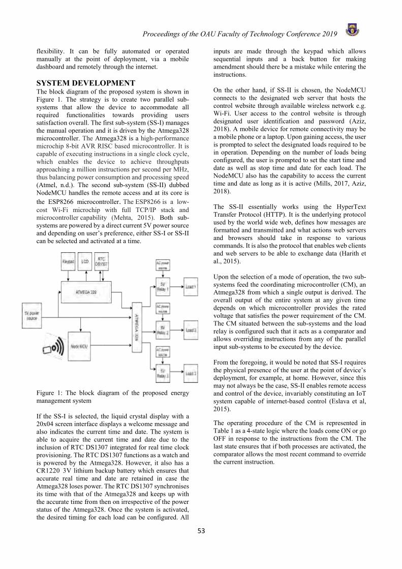
Proceedings of the OAU Faculty of Technology Conference 2019
53
flexibility. It can be fully automated or operated manually at the point of deployment, via a mobile dashboard and remotely through the internet.
SYSTEM DEVELOPMENT The block diagram of the proposed system is shown in Figure 1. The strategy is to create two parallel sub-systems that allow the device to accommodate all required functionalities towards providing users satisfaction overall. The first sub-system (SS-I) manages the manual operation and it is driven by the Atmega328 microcontroller. The Atmega328 is a high-performance microchip 8-bit AVR RISC based microcontroller. It is capable of executing instructions in a single clock cycle, which enables the device to achieve throughputs approaching a million instructions per second per MHz, thus balancing power consumption and processing speed (Atmel, n.d.). The second sub-system (SS-II) dubbed NodeMCU handles the remote access and at its core is the ESP8266 microcontroller. The ESP8266 is a low-cost Wi-Fi microchip with full TCP/IP stack and microcontroller capability (Mehta, 2015). Both sub-systems are powered by a direct current 5V power source and depending on user’s preference, either SS-I or SS-II can be selected and activated at a time.
Figure 1: The block diagram of the proposed energy management system
If the SS-I is selected, the liquid crystal display with a 20x04 screen interface displays a welcome message and also indicates the current time and date. The system is able to acquire the current time and date due to the inclusion of RTC DS1307 integrated for real time clock provisioning. The RTC DS1307 functions as a watch and is powered by the Atmega328. However, it also has a CR1220 3V lithium backup battery which ensures that accurate real time and date are retained in case the Atmega328 loses power. The RTC DS1307 synchronises its time with that of the Atmega328 and keeps up with the accurate time from then on irrespective of the power status of the Atmega328. Once the system is activated, the desired timing for each load can be configured. All
inputs are made through the keypad which allows sequential inputs and a back button for making amendment should there be a mistake while entering the instructions. On the other hand, if SS-II is chosen, the NodeMCU connects to the designated web server that hosts the control website through available wireless network e.g. Wi-Fi. User access to the control website is through designated user identification and password (Aziz, 2018). A mobile device for remote connectivity may be a mobile phone or a laptop. Upon gaining access, the user is prompted to select the designated loads required to be in operation. Depending on the number of loads being configured, the user is prompted to set the start time and date as well as stop time and date for each load. The NodeMCU also has the capability to access the current time and date as long as it is active (Mills, 2017, Aziz, 2018). The SS-II essentially works using the HyperText Transfer Protocol (HTTP). It is the underlying protocol used by the world wide web, defines how messages are formatted and transmitted and what actions web servers and browsers should take in response to various commands. It is also the protocol that enables web clients and web servers to be able to exchange data (Harith et al., 2015). Upon the selection of a mode of operation, the two sub-systems feed the coordinating microcontroller (CM), an Atmega328 from which a single output is derived. The overall output of the entire system at any given time depends on which microcontroller provides the rated voltage that satisfies the power requirement of the CM. The CM situated between the sub-systems and the load relay is configured such that it acts as a comparator and allows overriding instructions from any of the parallel input sub-systems to be executed by the device. From the foregoing, it would be noted that SS-I requires the physical presence of the user at the point of device’s deployment, for example, at home. However, since this may not always be the case, SS-II enables remote access and control of the device, invariably constituting an IoT system capable of internet-based control (Eslava et al, 2015). The operating procedure of the CM is represented in Table 1 as a 4-state logic where the loads come ON or go OFF in response to the instructions from the CM. The last state ensures that if both processes are activated, the comparator allows the most recent command to override the current instruction.
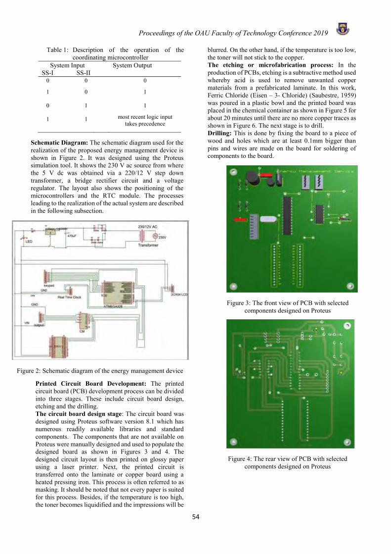
Proceedings of the OAU Faculty of Technology Conference 2019
54
Table 1: Description of the operation of the coordinating microcontroller
System Input SS-I SS-II
System Output
0 0
0
1 0 1
0 1 1 1 1
most recent logic input
takes precedence
Schematic Diagram: The schematic diagram used for the realization of the proposed energy management device is shown in Figure 2. It was designed using the Proteus simulation tool. It shows the 230 V ac source from where the 5 V dc was obtained via a 220/12 V step down transformer, a bridge rectifier circuit and a voltage regulator. The layout also shows the positioning of the microcontrollers and the RTC module. The processes leading to the realization of the actual system are described in the following subsection.
Figure 2: Schematic diagram of the energy management device
Printed Circuit Board Development: The printed circuit board (PCB) development process can be divided into three stages. These include circuit board design, etching and the drilling. The circuit board design stage: The circuit board was designed using Proteus software version 8.1 which has numerous readily available libraries and standard components. The components that are not available on Proteus were manually designed and used to populate the designed board as shown in Figures 3 and 4. The designed circuit layout is then printed on glossy paper using a laser printer. Next, the printed circuit is transferred onto the laminate or copper board using a heated pressing iron. This process is often referred to as masking. It should be noted that not every paper is suited for this process. Besides, if the temperature is too high, the toner becomes liquidified and the impressions will be
blurred. On the other hand, if the temperature is too low, the toner will not stick to the copper. The etching or microfabrication process: In the production of PCBs, etching is a subtractive method used whereby acid is used to remove unwanted copper materials from a prefabricated laminate. In this work, Ferric Chloride (Eisen – 3- Chloride) (Saubestre, 1959) was poured in a plastic bowl and the printed board was placed in the chemical container as shown in Figure 5 for about 20 minutes until there are no more copper traces as shown in Figure 6. The next stage is to drill. Drilling: This is done by fixing the board to a piece of wood and holes which are at least 0.1mm bigger than pins and wires are made on the board for soldering of components to the board.
Figure 3: The front view of PCB with selected components designed on Proteus
Figure 4: The rear view of PCB with selected components designed on Proteus

Proceedings of the OAU Faculty of Technology Conference 2019
55
(a) (b) Figure 5: Etching process after (a) 3 mins and (b) 7 mins
Figure 6: The printed circuit board after etching
RESULTS AND DISCUSSION Operation of sub-system I. The functionality of the developed system was investigated using three parallel loads that are controlled by separate relays. When the system was turned ON and operated in the SS-I mode, Figure 7 shows the initialization page that prompts the user to activate the device. This stage allows the user to confirm the mode of operation after which a welcome message appears, and the current time and date are displayed to allow the user to configure the loads as desired. This is indicated in Figures 8 and 9. Once the loads have all been configured and accepted by the system, the display alternately indicates the current loads status as shown in Figure 10.
Figure 7: The Initialization page
.
Figure 10: Operation page which notifies the user when the load is on based on the pre-set time
Operation of sub-system II. The deployment dashboard for SS-II at different stages of operation are as shown in Figures 11 and 12 using a laptop computer. In particular, Figure 11 shows the registration page which is immediately followed by the log-in page that facilitates user access. In Figure 12, the remote request submission page with the logs of all requests is shown.
Figure 8: Operation page prompting the user to set load hour start time
Figure 9: Operation page prompting the user to set load hour stop time
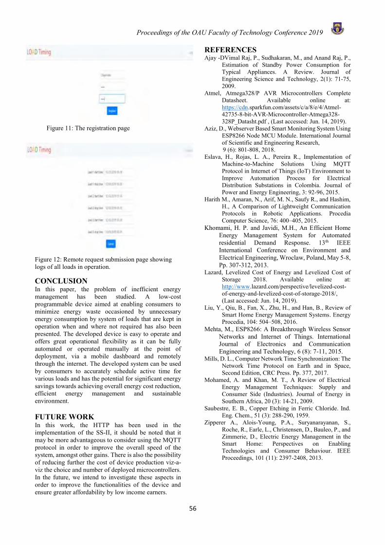
Proceedings of the OAU Faculty of Technology Conference 2019
56
Figure 11: The registration page
Figure 12: Remote request submission page showing logs of all loads in operation.
CONCLUSION In this paper, the problem of inefficient energy management has been studied. A low-cost programmable device aimed at enabling consumers to minimize energy waste occasioned by unnecessary energy consumption by system of loads that are kept in operation when and where not required has also been presented. The developed device is easy to operate and offers great operational flexibility as it can be fully automated or operated manually at the point of deployment, via a mobile dashboard and remotely through the internet. The developed system can be used by consumers to accurately schedule active time for various loads and has the potential for significant energy savings towards achieving overall energy cost reduction, efficient energy management and sustainable environment.
FUTURE WORK In this work, the HTTP has been used in the implementation of the SS-II, it should be noted that it may be more advantageous to consider using the MQTT protocol in order to improve the overall speed of the system, amongst other gains. There is also the possibility of reducing further the cost of device production viz-a-viz the choice and number of deployed microcontrollers. In the future, we intend to investigate these aspects in order to improve the functionalities of the device and ensure greater affordability by low income earners.
REFERENCES Ajay -DVimal Raj, P., Sudhakaran, M., and Anand Raj, P.,
Estimation of Standby Power Consumption for Typical Appliances. A Review. Journal of Engineering Science and Technology, 2(1): 71-75, 2009.
Atmel, Atmega328/P AVR Microcontrollers Complete Datasheet. Available online at: https://cdn.sparkfun.com/assets/c/a/8/e/4/Atmel-42735-8-bit-AVR-Microcontroller-Atmega328-328P_Datasht.pdf , (Last accessed: Jun. 14, 2019).
Aziz, D., Webserver Based Smart Monitoring System Using ESP8266 Node MCU Module. International Journal of Scientific and Engineering Research,
9 (6): 801-808, 2018. Eslava, H., Rojas, L. A., Pereira R., Implementation of
Machine-to-Machine Solutions Using MQTT Protocol in Internet of Things (IoT) Environment to Improve Automation Process for Electrical Distribution Substations in Colombia. Journal of Power and Energy Engineering, 3: 92-96, 2015.
Harith M., Amaran, N., Arif, M. N., Saufy R., and Hashim, H., A Comparison of Lightweight Communication Protocols in Robotic Applications. Procedia Computer Science, 76: 400–405, 2015.
Khomami, H. P. and Javidi, M.H., An Efficient Home Energy Management System for Automated residential Demand Response. 13th IEEE International Conference on Environment and Electrical Engineering, Wroclaw, Poland, May 5-8, Pp. 307-312, 2013.
Lazard, Levelized Cost of Energy and Levelized Cost of Storage 2018. Available online at: http://www.lazard.com/perspective/levelized-cost-of-energy-and-levelized-cost-of-storage-2018/, (Last accessed: Jun. 14, 2019).
Liu, Y., Qiu, B., Fan, X., Zhu, H., and Han, B., Review of Smart Home Energy Management Systems. Energy Procedia, 104: 504–508, 2016.
Mehta, M., ESP8266: A Breakthrough Wireless Sensor Networks and Internet of Things. International Journal of Electronics and Communication Engineering and Technology, 6 (8): 7-11, 2015.
Mills, D. L., Computer Network Time Synchronization: The Network Time Protocol on Earth and in Space, Second Edition, CRC Press. Pp. 377, 2017.
Mohamed, A. and Khan, M. T., A Review of Electrical Energy Management Techniques: Supply and Consumer Side (Industries). Journal of Energy in Southern Africa, 20 (3): 14-21, 2009.
Saubestre, E. B., Copper Etching in Ferric Chloride. Ind. Eng. Chem., 51 (3): 288-290, 1959.
Zipperer A., Alois-Young, P.A., Suryanarayanan, S., Roche, R., Earle, L., Christensen, D., Bauleo, P., and Zimmerie, D., Electric Energy Management in the Smart Home: Perspectives on Enabling Technologies and Consumer Behaviour. IEEE Proceedings, 101 (11): 2397-2408, 2013.
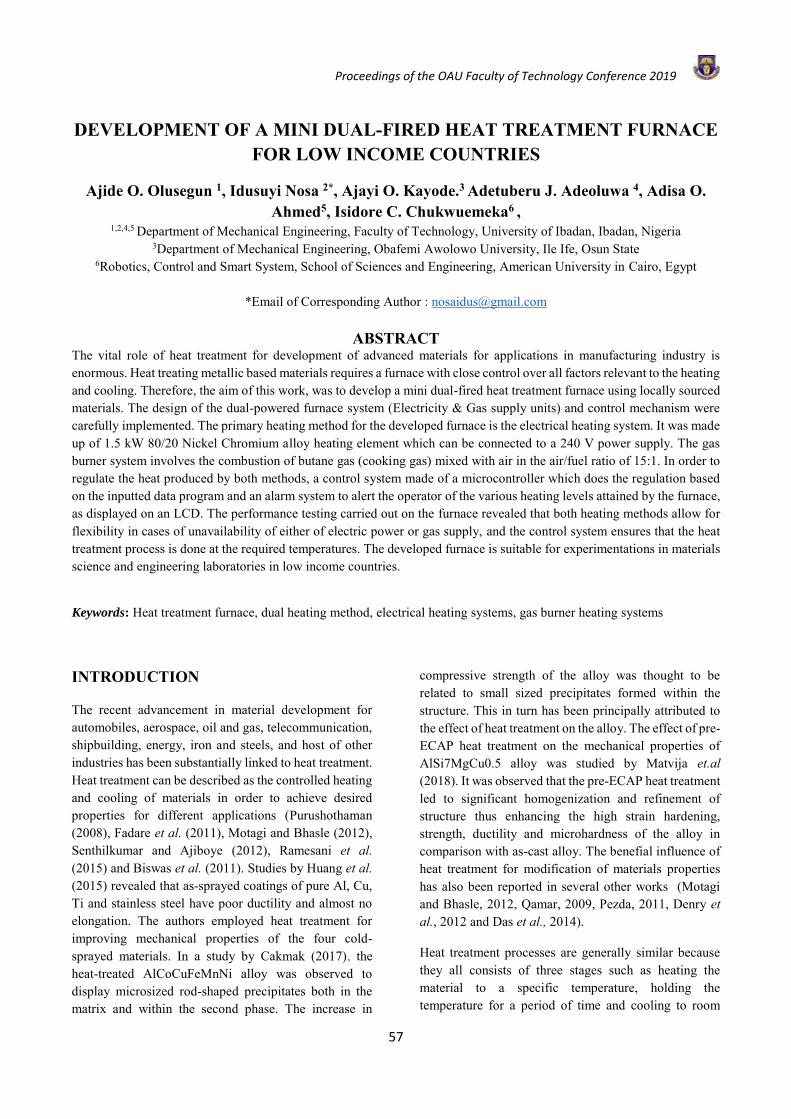
Proceedings of the OAU Faculty of Technology Conference 2019
57
DEVELOPMENT OF A MINI DUAL-FIRED HEAT TREATMENT FURNACE FOR LOW INCOME COUNTRIES
Ajide O. Olusegun 1, Idusuyi Nosa 2*, Ajayi O. Kayode.3 Adetuberu J. Adeoluwa 4, Adisa O. Ahmed5, Isidore C. Chukwuemeka6 ,
1,2,4,5 Department of Mechanical Engineering, Faculty of Technology, University of Ibadan, Ibadan, Nigeria 3Department of Mechanical Engineering, Obafemi Awolowo University, Ile Ife, Osun State
6Robotics, Control and Smart System, School of Sciences and Engineering, American University in Cairo, Egypt
*Email of Corresponding Author : [email protected]
ABSTRACT The vital role of heat treatment for development of advanced materials for applications in manufacturing industry is enormous. Heat treating metallic based materials requires a furnace with close control over all factors relevant to the heating and cooling. Therefore, the aim of this work, was to develop a mini dual-fired heat treatment furnace using locally sourced materials. The design of the dual-powered furnace system (Electricity & Gas supply units) and control mechanism were carefully implemented. The primary heating method for the developed furnace is the electrical heating system. It was made up of 1.5 kW 80/20 Nickel Chromium alloy heating element which can be connected to a 240 V power supply. The gas burner system involves the combustion of butane gas (cooking gas) mixed with air in the air/fuel ratio of 15:1. In order to regulate the heat produced by both methods, a control system made of a microcontroller which does the regulation based on the inputted data program and an alarm system to alert the operator of the various heating levels attained by the furnace, as displayed on an LCD. The performance testing carried out on the furnace revealed that both heating methods allow for flexibility in cases of unavailability of either of electric power or gas supply, and the control system ensures that the heat treatment process is done at the required temperatures. The developed furnace is suitable for experimentations in materials science and engineering laboratories in low income countries.
Keywords: Heat treatment furnace, dual heating method, electrical heating systems, gas burner heating systems
INTRODUCTION
The recent advancement in material development for automobiles, aerospace, oil and gas, telecommunication, shipbuilding, energy, iron and steels, and host of other industries has been substantially linked to heat treatment. Heat treatment can be described as the controlled heating and cooling of materials in order to achieve desired properties for different applications (Purushothaman (2008), Fadare et al. (2011), Motagi and Bhasle (2012), Senthilkumar and Ajiboye (2012), Ramesani et al. (2015) and Biswas et al. (2011). Studies by Huang et al. (2015) revealed that as-sprayed coatings of pure Al, Cu, Ti and stainless steel have poor ductility and almost no elongation. The authors employed heat treatment for improving mechanical properties of the four cold-sprayed materials. In a study by Cakmak (2017), the heat-treated AlCoCuFeMnNi alloy was observed to display microsized rod-shaped precipitates both in the matrix and within the second phase. The increase in
compressive strength of the alloy was thought to be related to small sized precipitates formed within the structure. This in turn has been principally attributed to the effect of heat treatment on the alloy. The effect of pre-ECAP heat treatment on the mechanical properties of AlSi7MgCu0.5 alloy was studied by Matvija et.al (2018). It was observed that the pre-ECAP heat treatment led to significant homogenization and refinement of structure thus enhancing the high strain hardening, strength, ductility and microhardness of the alloy in comparison with as-cast alloy. The benefial influence of heat treatment for modification of materials properties has also been reported in several other works (Motagi and Bhasle, 2012, Qamar, 2009, Pezda, 2011, Denry et al., 2012 and Das et al., 2014).
Heat treatment processes are generally similar because they all consists of three stages such as heating the material to a specific temperature, holding the temperature for a period of time and cooling to room
Proceedings of the OAU Faculty of Technology Conference 2019
58
temperature (Ismail et al., 2016). . However, there are differences in the methods used, such as the heating temperatures, cooling rates, and quenching media necessary to achieve the desired properties (Ramoliya et al. 2017). To heat treat a metallic based material, there is need to have a furnace with close control over all factors relevant to the heating and cooling. In the work of Purushothaman (2008), an attempt was made to develop a comprehensive furnace model by improving on the then available Computerized Heat Treatment (CHT) planning system-based furnace model. An enhanced furnace model based on Knowledge Data Discovery (KDD) technique and neural network was developed and validated in the author’s work. The model developed by the author was able to account for the real time furnace parameters determined from the experimental data. In addition, parameters capturing furnace deterioration and some of the complex heating patterns that occur inside the furnace. Ukoba et al. (2012) developed a low heat treatment furnace for ferrous, non-ferrous metals and their alloys. The developed furnace reached temperatures of 880°C in the furnace heating zone. Osarenwinda (2015) developed and evaluated an oil-fired crucible furnace using locally acquired materials. The developed furnace was observed to have a fast heating rate of 43.9°C /min and attained a temperature as high as 1386°C. Thus, it could be used for most metallic components. Jin (2015) incorporated programmable logical controllers to achieve automatic control of furnace temperature. The automation of the furnace system was found to effectively enhance heat treatment processing and overall production quality of 30CrMnSiA steel. Hoang et al. (2018) identified the poor performance of mechanical equipment arising from poor quality of welds. This was attributed to the presence of stresses in weldment before heat treatment, uneven microstructure and micro-segregation. Therefore, the authors successfully developed a small-scale heat treatment furnace capable of enhancing the microstructure of the welds and thus its mechanical properties. A diesel-powered heat-treatment furnace was developed by Alaneme and Olanrewaju (2010) using locally sourced materials. Due to epileptic power supply in Nigeria, the authors’ design philosophy was to eliminate the use of electric heating. The refractory blocks made from molten mixture of kaolin, clay, sawdust and water were used for lining the inner wall. Performance evaluation of the
furnace revealed a heating rate of 61.24 0C/min to attain a pre-set temperature of 9000°C, and a fuel consumption rate less than 1.4 1litres/hr. The developed furnace had good heat retaining capacity.
No nation can advance technologically, unless it is able to harness, convert its mineral resources and fabricate most of its equipment and machines locally (Osarewinda, 2015 and Bala, 2005). It is pertinent for developing countries like Nigeria to change the attitudes of near total dependence on foreign equipment and increase the stocks of locally developed ones. Therefore, attempt is made in the present work to develop a mini dual-fired heat treatment furnace for materials science and engineering laboratories in low income countries.
MATERIALS AND METHOD
The dual heating method heat treatment furnace is made up of the following:
Line Voltage of 240V/12V battery input LCD Display Microcontroller (PIC 16F877A) Keypad Heating Element: 1.5KW Nickel-Chromium
alloy Gas burner
The block diagram in Figure 1 shows the system breakdown,
The design analysis can be divided into four (3) sections: Electricity supply design, Gas supply design, and Control mechanism design.
Electrical Supply/Electronic Design Figure 2 shows the block diagram for the Electronic unit design. Here, the power supply is from the 240V AC mains, and is stepped down to 5V with the help of a transformer, which is the operating voltage of the microcontroller.
Transformer: A step down transformer was used in this project to bring down the voltage from 240V to 5V and from 12V to 5V.

Proceedings of the OAU Faculty of Technology Conference 2019
59
Figure 1: Block Diagram showing the system breakdown
Figure 2: Block diagram of the AC Mode power source design
Buzzer: The buzzer was used to send an indication to the operator, immediately the power gets into the panel and when the furnace temperature reaches the desired value.
Heating Element: The 80/20 Nickel-chromium alloy was used for this purpose.
Gas Power Supply Design
Figure 3 shows the block diagram for the design of the gas supply unit.
This implies that for a complete combustion of the gas, every 1kg of fuel will require 15.5kg of air.
Gas Burner: The Gas burner was designed using mild steel, it consisted of a blower to regulate the type of flame and eliminate incomplete combustion as much as possible. The gas burner had the following components: 1” pipe (10” in length), Gas Hose, Squirrel cage fan, Mild steel, 12V motor, Gas Regulator. The CAD diagram in Figure 4 and Figure 5 shows the arrangement of the gas burner.
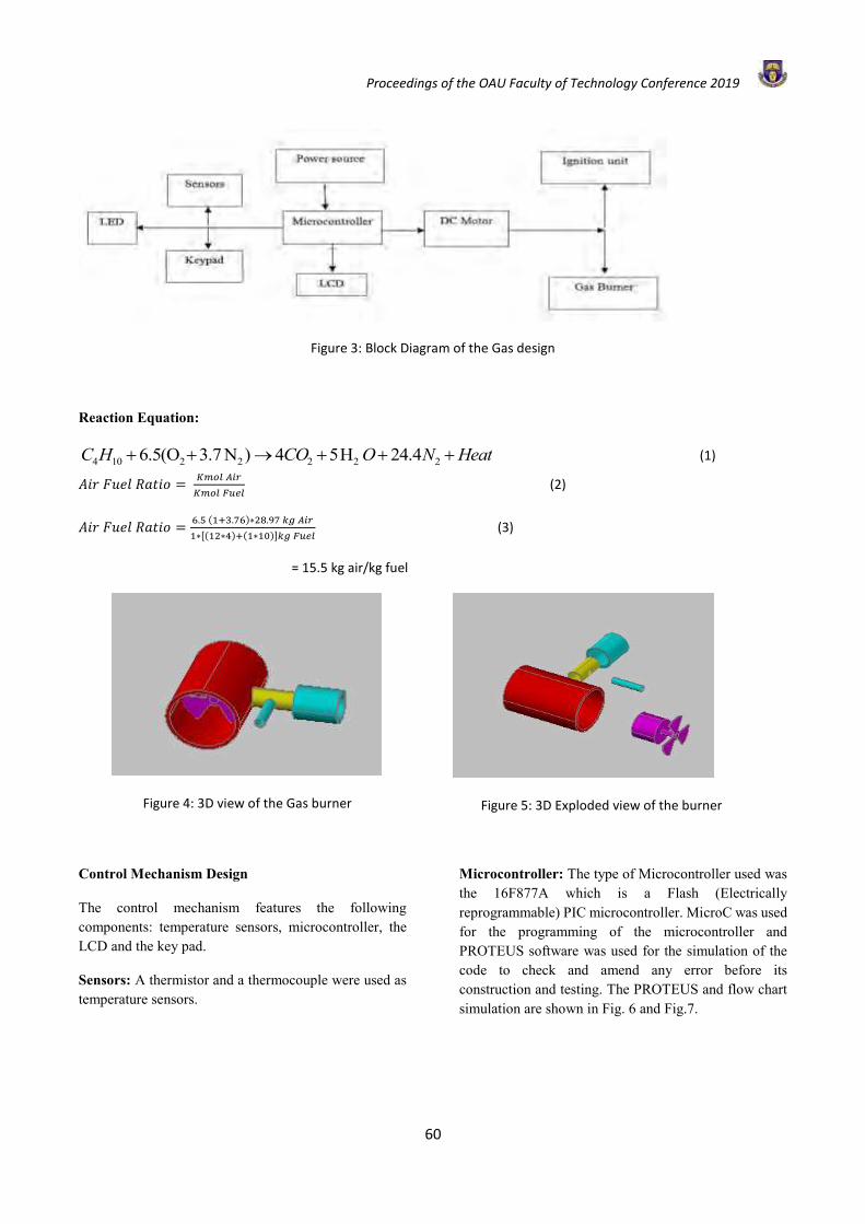
Proceedings of the OAU Faculty of Technology Conference 2019
60
Figure 3: Block Diagram of the Gas design
Reaction Equation:
4 10 2 2 2 2 26.5(O 3.7 N ) 4 5H 24.4C H CO O N Heat+ + → + + + (1)
𝐴𝑖𝑟 𝐹𝑢𝑒𝑙 𝑅𝑎𝑡𝑖𝑜 = 𝐾𝑚𝑜𝑙 𝐴𝑖𝑟
𝐾𝑚𝑜𝑙 𝐹𝑢𝑒𝑙 (2)
𝐴𝑖𝑟 𝐹𝑢𝑒𝑙 𝑅𝑎𝑡𝑖𝑜 =6.5 (1+3.76)∗28.97 𝑘𝑔 𝐴𝑖𝑟
1∗[(12∗4)+(1∗10)]𝑘𝑔 𝐹𝑢𝑒𝑙 (3)
= 15.5 kg air/kg fuel
Figure 4: 3D view of the Gas burner
Figure 5: 3D Exploded view of the burner
Control Mechanism Design
The control mechanism features the following components: temperature sensors, microcontroller, the LCD and the key pad.
Sensors: A thermistor and a thermocouple were used as temperature sensors.
Microcontroller: The type of Microcontroller used was the 16F877A which is a Flash (Electrically reprogrammable) PIC microcontroller. MicroC was used for the programming of the microcontroller and PROTEUS software was used for the simulation of the code to check and amend any error before its construction and testing. The PROTEUS and flow chart simulation are shown in Fig. 6 and Fig.7.
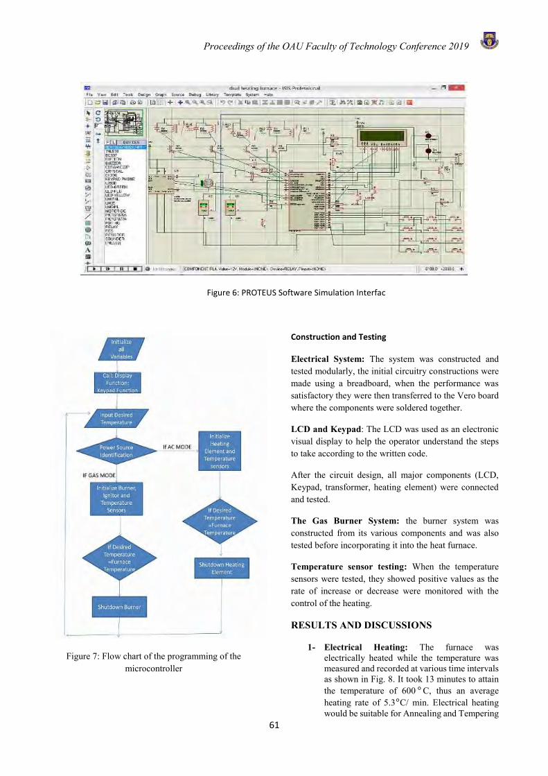
Proceedings of the OAU Faculty of Technology Conference 2019
61
Figure 6: PROTEUS Software Simulation Interfac
Figure 7: Flow chart of the programming of the microcontroller
Construction and Testing
Electrical System: The system was constructed and tested modularly, the initial circuitry constructions were made using a breadboard, when the performance was satisfactory they were then transferred to the Vero board where the components were soldered together.
LCD and Keypad: The LCD was used as an electronic visual display to help the operator understand the steps to take according to the written code.
After the circuit design, all major components (LCD, Keypad, transformer, heating element) were connected and tested.
The Gas Burner System: the burner system was constructed from its various components and was also tested before incorporating it into the heat furnace.
Temperature sensor testing: When the temperature sensors were tested, they showed positive values as the rate of increase or decrease were monitored with the control of the heating.
RESULTS AND DISCUSSIONS
1- Electrical Heating: The furnace was electrically heated while the temperature was measured and recorded at various time intervals as shown in Fig. 8. It took 13 minutes to attain the temperature of 600 ° C, thus an average heating rate of 5.3°C/ min. Electrical heating would be suitable for Annealing and Tempering
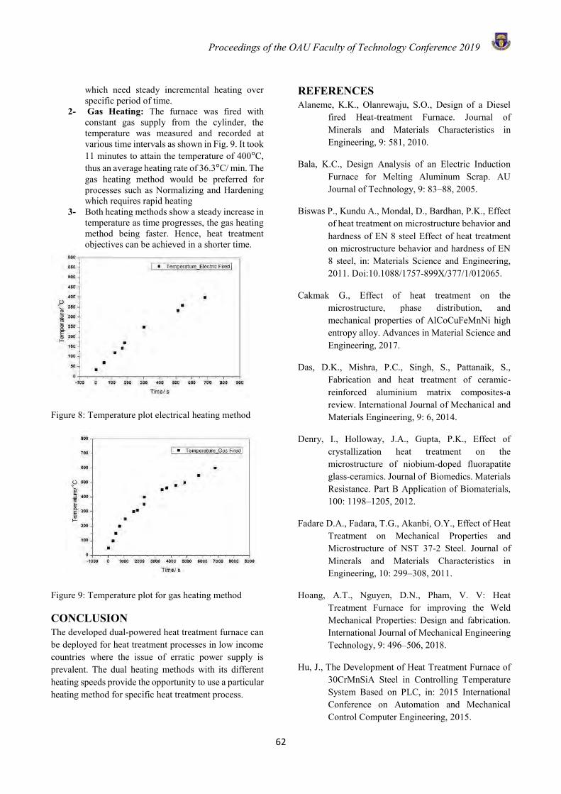
Proceedings of the OAU Faculty of Technology Conference 2019
62
which need steady incremental heating over specific period of time.
2- Gas Heating: The furnace was fired with constant gas supply from the cylinder, the temperature was measured and recorded at various time intervals as shown in Fig. 9. It took 11 minutes to attain the temperature of 400°C, thus an average heating rate of 36.3°C/ min. The gas heating method would be preferred for processes such as Normalizing and Hardening which requires rapid heating
3- Both heating methods show a steady increase in temperature as time progresses, the gas heating method being faster. Hence, heat treatment objectives can be achieved in a shorter time.
Figure 8: Temperature plot electrical heating method
Figure 9: Temperature plot for gas heating method
CONCLUSION The developed dual-powered heat treatment furnace can be deployed for heat treatment processes in low income countries where the issue of erratic power supply is prevalent. The dual heating methods with its different heating speeds provide the opportunity to use a particular heating method for specific heat treatment process.
REFERENCES Alaneme, K.K., Olanrewaju, S.O., Design of a Diesel
fired Heat-treatment Furnace. Journal of Minerals and Materials Characteristics in Engineering, 9: 581, 2010.
Bala, K.C., Design Analysis of an Electric Induction Furnace for Melting Aluminum Scrap. AU Journal of Technology, 9: 83–88, 2005.
Biswas P., Kundu A., Mondal, D., Bardhan, P.K., Effect of heat treatment on microstructure behavior and hardness of EN 8 steel Effect of heat treatment on microstructure behavior and hardness of EN 8 steel, in: Materials Science and Engineering, 2011. Doi:10.1088/1757-899X/377/1/012065.
Cakmak G., Effect of heat treatment on the microstructure, phase distribution, and mechanical properties of AlCoCuFeMnNi high entropy alloy. Advances in Material Science and Engineering, 2017.
Das, D.K., Mishra, P.C., Singh, S., Pattanaik, S., Fabrication and heat treatment of ceramic-reinforced aluminium matrix composites-a review. International Journal of Mechanical and Materials Engineering, 9: 6, 2014.
Denry, I., Holloway, J.A., Gupta, P.K., Effect of crystallization heat treatment on the microstructure of niobium-doped fluorapatite glass-ceramics. Journal of Biomedics. Materials Resistance. Part B Application of Biomaterials, 100: 1198–1205, 2012.
Fadare D.A., Fadara, T.G., Akanbi, O.Y., Effect of Heat Treatment on Mechanical Properties and Microstructure of NST 37-2 Steel. Journal of Minerals and Materials Characteristics in Engineering, 10: 299–308, 2011.
Hoang, A.T., Nguyen, D.N., Pham, V. V: Heat Treatment Furnace for improving the Weld Mechanical Properties: Design and fabrication. International Journal of Mechanical Engineering Technology, 9: 496–506, 2018.
Hu, J., The Development of Heat Treatment Furnace of 30CrMnSiA Steel in Controlling Temperature System Based on PLC, in: 2015 International Conference on Automation and Mechanical Control Computer Engineering, 2015.
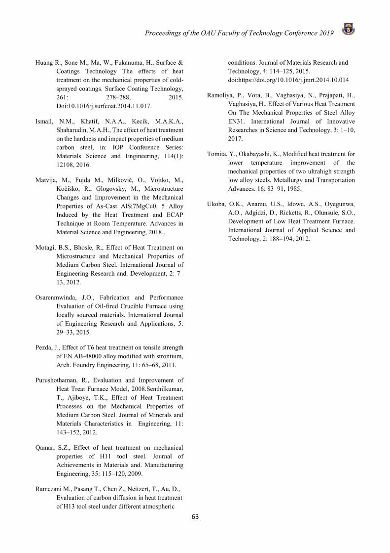
Proceedings of the OAU Faculty of Technology Conference 2019
63
Huang R., Sone M., Ma, W., Fukanuma, H., Surface & Coatings Technology The effects of heat treatment on the mechanical properties of cold-sprayed coatings. Surface Coating Technology, 261: 278–288, 2015. Doi:10.1016/j.surfcoat.2014.11.017.
Ismail, N.M., Khatif, N.A.A., Kecik, M.A.K.A., Shaharudin, M.A.H., The effect of heat treatment on the hardness and impact properties of medium carbon steel, in: IOP Conference Series: Materials Science and Engineering, 114(1): 12108, 2016.
Matvija, M., Fujda M., Milkovič, O., Vojtko, M., Kočiško, R., Glogovsky, M., Microstructure Changes and Improvement in the Mechanical Properties of As-Cast AlSi7MgCu0. 5 Alloy Induced by the Heat Treatment and ECAP Technique at Room Temperature. Advances in Material Science and Engineering, 2018..
Motagi, B.S., Bhosle, R., Effect of Heat Treatment on Microstructure and Mechanical Properties of Medium Carbon Steel. International Journal of Engineering Research and. Development, 2: 7–13, 2012.
Osarenmwinda, J.O., Fabrication and Performance Evaluation of Oil-fired Crucible Furnace using locally sourced materials. International Journal of Engineering Research and Applications, 5: 29–33, 2015.
Pezda, J., Effect of T6 heat treatment on tensile strength of EN AB-48000 alloy modified with strontium, Arch. Foundry Engineering, 11: 65–68, 2011.
Purushothaman, R., Evaluation and Improvement of Heat Treat Furnace Model, 2008.Senthilkumar, T., Ajiboye, T.K., Effect of Heat Treatment Processes on the Mechanical Properties of Medium Carbon Steel. Journal of Minerals and Materials Characteristics in Engineering, 11: 143–152, 2012.
Qamar, S.Z., Effect of heat treatment on mechanical properties of H11 tool steel. Journal of Achievements in Materials and. Manufacturing Engineering, 35: 115–120, 2009.
Ramezani M., Pasang T., Chen Z., Neitzert, T., Au, D., Evaluation of carbon diffusion in heat treatment of H13 tool steel under different atmospheric
conditions. Journal of Materials Research and Technology, 4: 114–125, 2015. doi:https://doi.org/10.1016/j.jmrt.2014.10.014
Ramoliya, P., Vora, B., Vaghasiya, N., Prajapati, H., Vaghasiya, H., Effect of Various Heat Treatment On The Mechanical Properties of Steel Alloy EN31. International Journal of Innovative Researches in Science and Technology, 3: 1–10, 2017.
Tomita, Y., Okabayashi, K., Modified heat treatment for lower temperature improvement of the mechanical properties of two ultrahigh strength low alloy steels. Metallurgy and Transportation Advances. 16: 83–91, 1985.
Ukoba, O.K., Anamu, U.S., Idowu, A.S., Oyegunwa, A.O., Adgidzi, D., Ricketts, R., Olunsule, S.O., Development of Low Heat Treatment Furnace. International Journal of Applied Science and Technology, 2: 188–194, 2012.
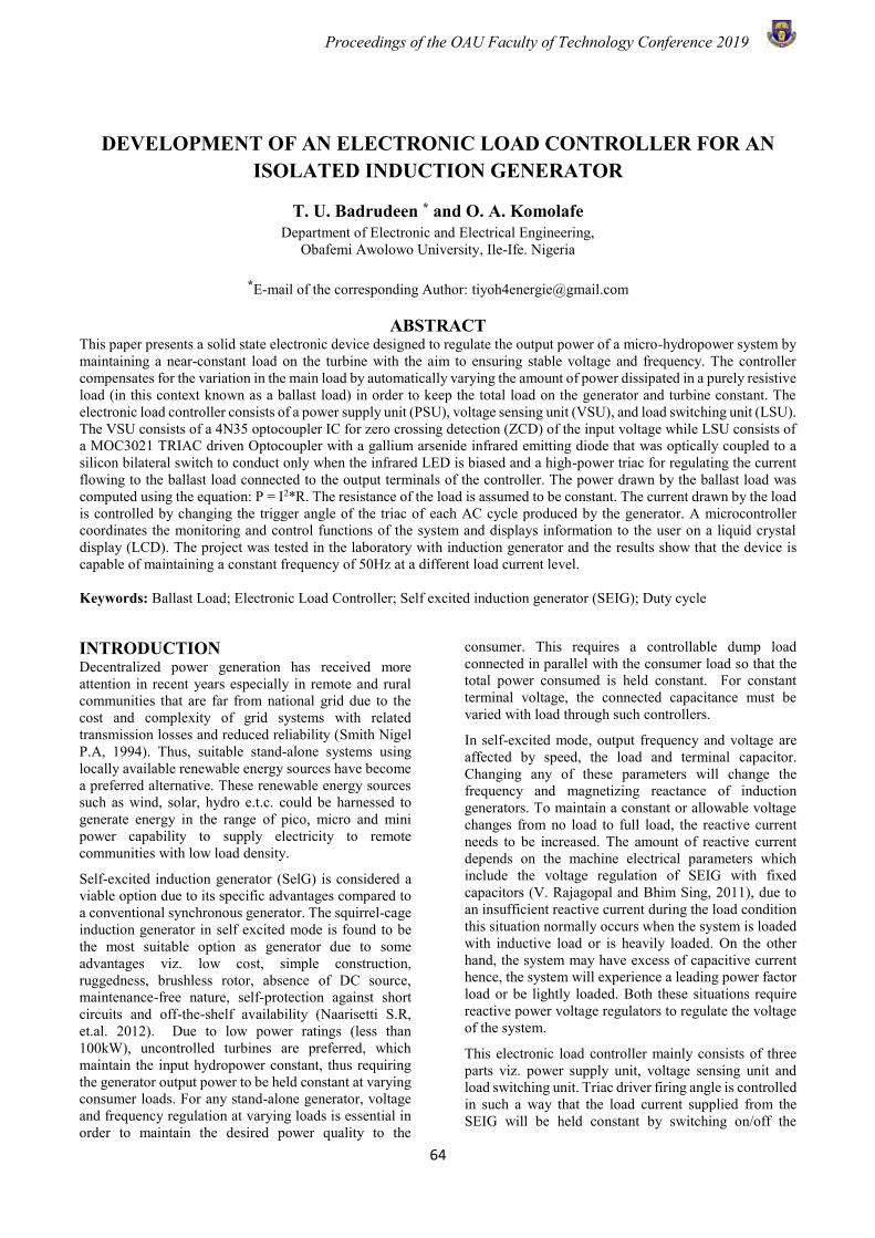
Proceedings of the OAU Faculty of Technology Conference 2019
64
DEVELOPMENT OF AN ELECTRONIC LOAD CONTROLLER FOR AN ISOLATED INDUCTION GENERATOR
T. U. Badrudeen * and O. A. Komolafe Department of Electronic and Electrical Engineering,
Obafemi Awolowo University, Ile-Ife. Nigeria
*E-mail of the corresponding Author: [email protected]
ABSTRACT This paper presents a solid state electronic device designed to regulate the output power of a micro-hydropower system by maintaining a near-constant load on the turbine with the aim to ensuring stable voltage and frequency. The controller compensates for the variation in the main load by automatically varying the amount of power dissipated in a purely resistive load (in this context known as a ballast load) in order to keep the total load on the generator and turbine constant. The electronic load controller consists of a power supply unit (PSU), voltage sensing unit (VSU), and load switching unit (LSU). The VSU consists of a 4N35 optocoupler IC for zero crossing detection (ZCD) of the input voltage while LSU consists of a MOC3021 TRIAC driven Optocoupler with a gallium arsenide infrared emitting diode that was optically coupled to a silicon bilateral switch to conduct only when the infrared LED is biased and a high-power triac for regulating the current flowing to the ballast load connected to the output terminals of the controller. The power drawn by the ballast load was computed using the equation: P = I2*R. The resistance of the load is assumed to be constant. The current drawn by the load is controlled by changing the trigger angle of the triac of each AC cycle produced by the generator. A microcontroller coordinates the monitoring and control functions of the system and displays information to the user on a liquid crystal display (LCD). The project was tested in the laboratory with induction generator and the results show that the device is capable of maintaining a constant frequency of 50Hz at a different load current level. Keywords: Ballast Load; Electronic Load Controller; Self excited induction generator (SEIG); Duty cycle
INTRODUCTION Decentralized power generation has received more attention in recent years especially in remote and rural communities that are far from national grid due to the cost and complexity of grid systems with related transmission losses and reduced reliability (Smith Nigel P.A, 1994). Thus, suitable stand-alone systems using locally available renewable energy sources have become a preferred alternative. These renewable energy sources such as wind, solar, hydro e.t.c. could be harnessed to generate energy in the range of pico, micro and mini power capability to supply electricity to remote communities with low load density.
Self-excited induction generator (SelG) is considered a viable option due to its specific advantages compared to a conventional synchronous generator. The squirrel-cage induction generator in self excited mode is found to be the most suitable option as generator due to some advantages viz. low cost, simple construction, ruggedness, brushless rotor, absence of DC source, maintenance-free nature, self-protection against short circuits and off-the-shelf availability (Naarisetti S.R, et.al. 2012). Due to low power ratings (less than 100kW), uncontrolled turbines are preferred, which maintain the input hydropower constant, thus requiring the generator output power to be held constant at varying consumer loads. For any stand-alone generator, voltage and frequency regulation at varying loads is essential in order to maintain the desired power quality to the
consumer. This requires a controllable dump load connected in parallel with the consumer load so that the total power consumed is held constant. For constant terminal voltage, the connected capacitance must be varied with load through such controllers.
In self-excited mode, output frequency and voltage are affected by speed, the load and terminal capacitor. Changing any of these parameters will change the frequency and magnetizing reactance of induction generators. To maintain a constant or allowable voltage changes from no load to full load, the reactive current needs to be increased. The amount of reactive current depends on the machine electrical parameters which include the voltage regulation of SEIG with fixed capacitors (V. Rajagopal and Bhim Sing, 2011), due to an insufficient reactive current during the load condition this situation normally occurs when the system is loaded with inductive load or is heavily loaded. On the other hand, the system may have excess of capacitive current hence, the system will experience a leading power factor load or be lightly loaded. Both these situations require reactive power voltage regulators to regulate the voltage of the system.
This electronic load controller mainly consists of three parts viz. power supply unit, voltage sensing unit and load switching unit. Triac driver firing angle is controlled in such a way that the load current supplied from the SEIG will be held constant by switching on/off the
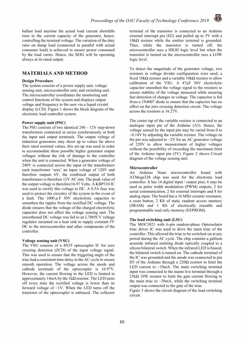
Proceedings of the OAU Faculty of Technology Conference 2019
65
ballast load anytime the actual load current shortfalls rises to the current capacity of the generator, hence; controlling the terminal voltage. The variation of the duty ratio on dump load (connected in parallel with actual consumer load) is achieved to ensure power consumed by the load varies. Hence, the SEIG will be operating always at its rated output.
MATERIALS AND METHOD Design Procedure The system consists of a power supply unit, voltage sensing unit, microcontroller unit, and switching unit. The microcontroller coordinates the monitoring and control functions of the system and displays output voltage and frequency to the user via a liquid crystal display (LCD). Figure 1 shows the block diagram of the electronic load controller system.
Power supply unit (PSU) The PSU consists of two identical 240 – 12V step-down transformers connected in series synchronously at both the input and output terminals. The output voltage of induction generators may shoot up to values far above their rated nominal values, this set-up was used in order to accommodate these possible higher generator output voltages without the risk of damage to the controller when the unit is connected. When a generator voltage of 240V is connected across the input of the transformers each transformer ‘sees’ an input voltage of 120V and therefore outputs 6V, the combined output of both transformers is therefore 12V AC rms. The peak value of the output voltage is therefore16.97 Volts. A KBP310 IC was used to rectify this voltage to DC. A 0.5A fuse was used to protect the circuitry of the system in the event of a fault. The 1000 𝜇 F 50V electrolytic capacitor to smoothen the ripples from the rectified DC voltage. The diode ensures that the voltage of the charged electrolytic capacitor does not affect the voltage sensing unit. The smoothened DC voltage was fed to an L7805CV voltage regulator mounted on a heat sink to supply constant 5V DC to the microcontroller and other components of the controller. Voltage sensing unit (VSU) The VSU consists of a 4N35 optocoupler IC for zero crossing detection (ZCD) of the input voltage signal. This was used to ensure that the triggering angle of the triac had a consistent time delay in the AC cycle to ensure smooth operation. The voltage across the anode and cathode terminals of the optocoupler is 16.97V. However, the current flowing to the LED is limited to approximately 14mA by the 1kΩ resistor. The LED turns off every time the rectified voltage is lower than its forward voltage of ~1V. When the LED turns off the transistor of the optocoupler is unbiased. The collector
terminal of the transistor is connected to an Arduino external interrupt pin (D2) and pulled up to 5V with a 10kΩ resistor while the emitter terminal is grounded. Thus, while the transistor is turned off, the microcontroller sees a HIGH logic level but when the transistor is turned on the microcontroller sees a LOW logic level. To detect the magnitude of the generator voltage, two resistors in voltage divider configuration were used; a fixed 10kΩ resistor and a variable 10kΩ resistor to allow calibration of the VSU. A 47μF 50V electrolytic capacitor smoothen the voltage signal to the resistors to ensure stability of the voltage measured while ensuring fast detection of changes in voltage. The capacitor is fed from a 1N4007 diode to ensure that the capacitor has no effect on the zero crossing detection circuit. The voltage across the resistors is 16.27V. The centre tap of the variable resistor is connected to an analogue input pin of the Arduino (A3). Hence, the voltage sensed by the input pin may be varied from 0 to ~8.14V by adjusting the variable resistor. The voltage on the pin was adjusted to ~2V for an AC generator voltage of 220V to allow measurement of higher voltages without the possibility of exceeding the maximum limit of the Arduino input pin (5V). Figure 2 shows Circuit diagram of the voltage sensing unit. Microcontroller An Arduino Nano microcontroller board with ATMega328 chip was used for the electronic load controller. It has 14 digital input / output pins; 6 may be used as pulse width modulation (PWM) outputs, 2 for serial communication, 2 for external interrupts and 8 for analog input. The board has a 16 MHz ceramic resonator, a reset button, 2 Kb of static random access memory (SRAM) and 1 Kb of electrically erasable and programmable read only memory (EEPROM).
The load switching unit (LSU) The MOC3021 with 6-pin random-phase Optoisolator triac driver IC was used to drive the main triac of the controller. This allowed the triac to be switched-on at any period during the AC cycle. The chip contains a gallium arsenide infrared emitting diode optically coupled to a silicon bilateral switch. When the infrared LED is biased, the bilateral switch is turned on. The cathode terminal of the IC was grounded and the anode was connected to pin D3 of the Arduino through a 220Ω resistor to limit the LED current to ~10mA. The main switching terminal input was connected to the mains live terminal through a 25kΩ 10W resistor to limit the gate current flowing to the main triac to ~30mA, while the switching terminal output was connected to the gate of the triac Figure 3 shows the circuit diagram of the load switching circuit.
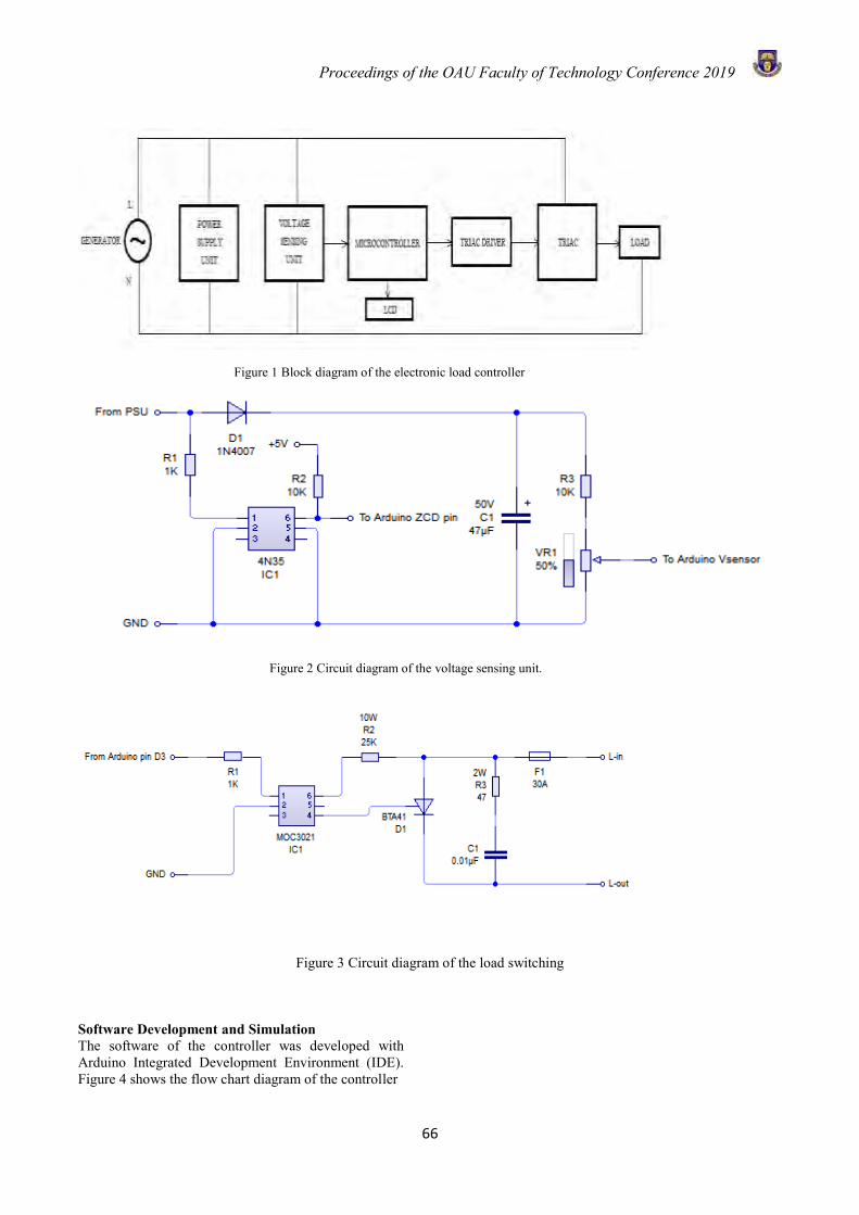
Proceedings of the OAU Faculty of Technology Conference 2019
66
Figure 1 Block diagram of the electronic load controller
Figure 2 Circuit diagram of the voltage sensing unit.
Figure 3 Circuit diagram of the load switching
Software Development and Simulation The software of the controller was developed with Arduino Integrated Development Environment (IDE). Figure 4 shows the flow chart diagram of the controller
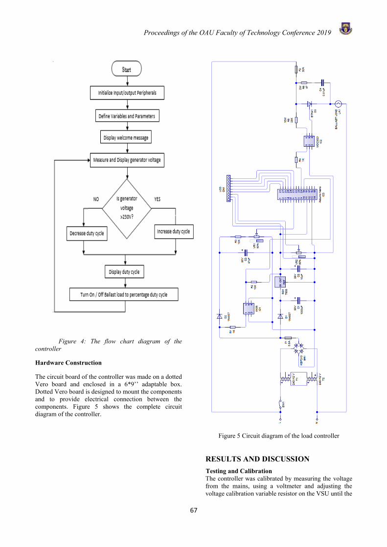
Proceedings of the OAU Faculty of Technology Conference 2019
67
Figure 4: The flow chart diagram of the controller
Hardware Construction
The circuit board of the controller was made on a dotted Vero board and enclosed in a 6*9’’ adaptable box. Dotted Vero board is designed to mount the components and to provide electrical connection between the components. Figure 5 shows the complete circuit diagram of the controller.
Figure 5 Circuit diagram of the load controller
RESULTS AND DISCUSSION Testing and Calibration The controller was calibrated by measuring the voltage from the mains, using a voltmeter and adjusting the voltage calibration variable resistor on the VSU until the
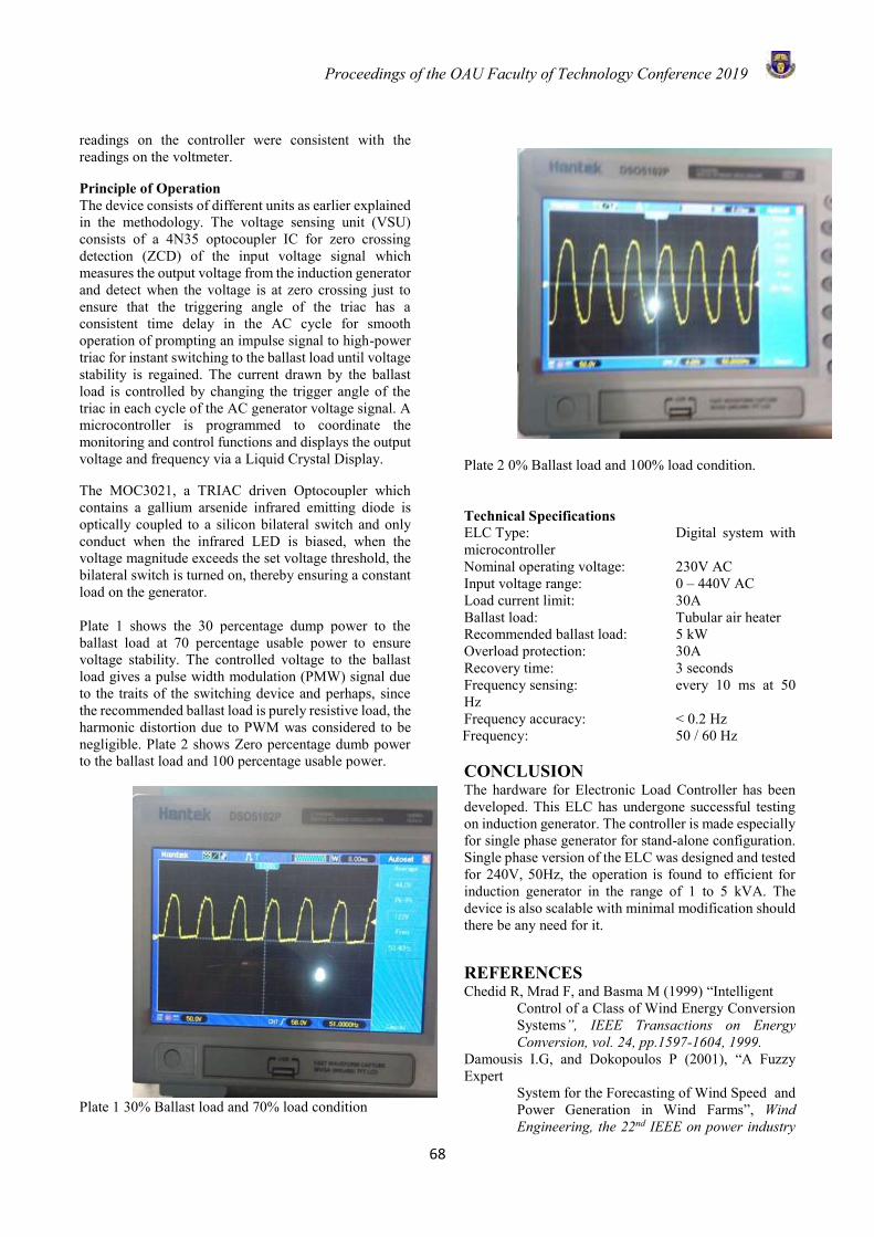
Proceedings of the OAU Faculty of Technology Conference 2019
68
readings on the controller were consistent with the readings on the voltmeter.
Principle of Operation The device consists of different units as earlier explained in the methodology. The voltage sensing unit (VSU) consists of a 4N35 optocoupler IC for zero crossing detection (ZCD) of the input voltage signal which measures the output voltage from the induction generator and detect when the voltage is at zero crossing just to ensure that the triggering angle of the triac has a consistent time delay in the AC cycle for smooth operation of prompting an impulse signal to high-power triac for instant switching to the ballast load until voltage stability is regained. The current drawn by the ballast load is controlled by changing the trigger angle of the triac in each cycle of the AC generator voltage signal. A microcontroller is programmed to coordinate the monitoring and control functions and displays the output voltage and frequency via a Liquid Crystal Display.
The MOC3021, a TRIAC driven Optocoupler which contains a gallium arsenide infrared emitting diode is optically coupled to a silicon bilateral switch and only conduct when the infrared LED is biased, when the voltage magnitude exceeds the set voltage threshold, the bilateral switch is turned on, thereby ensuring a constant load on the generator. Plate 1 shows the 30 percentage dump power to the ballast load at 70 percentage usable power to ensure voltage stability. The controlled voltage to the ballast load gives a pulse width modulation (PMW) signal due to the traits of the switching device and perhaps, since the recommended ballast load is purely resistive load, the harmonic distortion due to PWM was considered to be negligible. Plate 2 shows Zero percentage dumb power to the ballast load and 100 percentage usable power.
Plate 1 30% Ballast load and 70% load condition
Plate 2 0% Ballast load and 100% load condition.
Technical Specifications ELC Type: Digital system with microcontroller Nominal operating voltage: 230V AC Input voltage range: 0 – 440V AC Load current limit: 30A Ballast load: Tubular air heater Recommended ballast load: 5 kW Overload protection: 30A Recovery time: 3 seconds Frequency sensing: every 10 ms at 50 Hz Frequency accuracy: < 0.2 Hz
Frequency: 50 / 60 Hz CONCLUSION The hardware for Electronic Load Controller has been developed. This ELC has undergone successful testing on induction generator. The controller is made especially for single phase generator for stand-alone configuration. Single phase version of the ELC was designed and tested for 240V, 50Hz, the operation is found to efficient for induction generator in the range of 1 to 5 kVA. The device is also scalable with minimal modification should there be any need for it.
REFERENCES Chedid R, Mrad F, and Basma M (1999) “Intelligent
Control of a Class of Wind Energy Conversion Systems”, IEEE Transactions on Energy Conversion, vol. 24, pp.1597-1604, 1999.
Damousis I.G, and Dokopoulos P (2001), “A Fuzzy Expert
System for the Forecasting of Wind Speed and Power Generation in Wind Farms”, Wind Engineering, the 22nd IEEE on power industry

Proceedings of the OAU Faculty of Technology Conference 2019
69
computer Application (PICA) Sydney, vol. 43, pp. 1-11, 2001.
Doolla S. and Bhatti T. S. (2006), “Load frequency control
of an isolated small hydropower plant with reduced dump load,” IEEE Transactions on Power Systems, vol.21, pp. 1912 – 1919, Dec. 2006.
Kanellos F.D and Hatziargyriou N.D (2012), “A New Control Scheme for Variable Speed Wind Turbines using Neural Networks”, IEEE Transactions on Energy Conversion, vol.14 pp. 181-186, 2012.
Khela R S, Bansal, Raj Kumar, Sandhu, K.S, Goel and Ashok Kumar.(2006)”Application of Artificial Neural Network for Analysis of Self-Excited Induction Generator”, Journal of Computer Science and Technology, vol.6 ,NO: 2. Pp. 73-79.2006.
Gaber Shabib and Youssef A. Mobarak (2012), “Coordinated Design of A Mb-Pss and Statcom controller To Enhance Power System Stability” International Journal of Electrical Engineering & Technology (IJEET), Vol. 3,Issue 2, , pp. 352 – 372, Sept, 2012.
Khela R S, Bansal, Raj Kumar, Sandhu, K.S, Goel and
Ashok Kumar.(2006)”Application of Artificial Neural Network for Analysis of Self-Excited Induction Generator”, Journal of Computer Science and Technology, vol.6 ,NO: 2. Pp. 73-79.2006.
69 nalyse A, and Sathish kumar G(2006) , “A Generalized
State-Space Modeling of Three phase self-excited induction generator for dynamic characteristics and analysis” Journal of Power Sources, vol.4, pp1-6,Aug. 2006.
Palwalia, D.K. and Singh S.P. (2008).”Design and Implementation of Induction Generator Controller for Single Phase Self Excited Induction Generator”. Industrial electronics and application, ICIEA 2008, 3rd IEEE conference, pp.400-404.
Bonetrt R. and Rajakaruna, S. “Self-excited induction generator with excellent voltage and frequency control,” in Electrical Engineering Transaction , vol. 145, no. 1, pp. 33–39, Jan. 1998.
Rajagopal V. and Bhim Sing (2011) “Improved Electronic
load controller for off grid induction generator in small hydropower generation” in Proc. Of 2010 India International Conference on Power Electronics (IICPE), New Delhi (India), Jan, 28-30. 2011, PP.1-7.
Robinson.L and Holmes.D.G (2006).” A Single Phase Self-
Excited Induction Generator with Voltage and Frequency Regulation for use in a remote Area
Power Supply”. Proc. Australasian Universities Power Engineering Conf. (AUPEC) Dec; 10-13, 2006 .
Naarisetti Srinivasa Rao and Dasam Srinivas, (2012) “An
Experimental Design To Improve Power Quality On Statcom” International Journal of Electrical Engineering & Technology (IJEET), ISSN , Vol. 4, issue 5, pp.96 – 103, 2012.
Smith Nigel P.A. (1994),” Induction Generator for Standalone Micro Hydro System”. Intermediate Technology Development Group, 1st Edition, pp1-90.
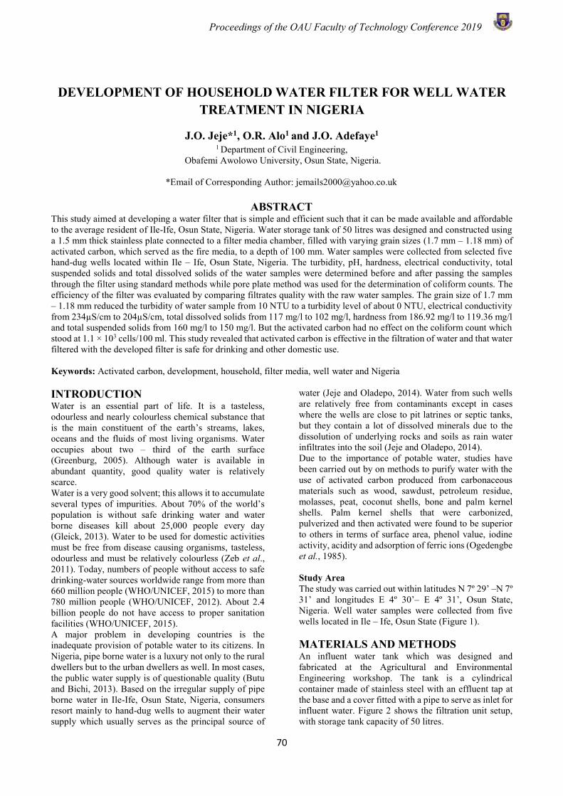
Proceedings of the OAU Faculty of Technology Conference 2019
70
DEVELOPMENT OF HOUSEHOLD WATER FILTER FOR WELL WATER TREATMENT IN NIGERIA
J.O. Jeje*1, O.R. Alo1 and J.O. Adefaye1 1 Department of Civil Engineering,
Obafemi Awolowo University, Osun State, Nigeria.
*Email of Corresponding Author: [email protected]
ABSTRACT This study aimed at developing a water filter that is simple and efficient such that it can be made available and affordable to the average resident of Ile-Ife, Osun State, Nigeria. Water storage tank of 50 litres was designed and constructed using a 1.5 mm thick stainless plate connected to a filter media chamber, filled with varying grain sizes (1.7 mm – 1.18 mm) of activated carbon, which served as the fire media, to a depth of 100 mm. Water samples were collected from selected five hand-dug wells located within Ile – Ife, Osun State, Nigeria. The turbidity, pH, hardness, electrical conductivity, total suspended solids and total dissolved solids of the water samples were determined before and after passing the samples through the filter using standard methods while pore plate method was used for the determination of coliform counts. The efficiency of the filter was evaluated by comparing filtrates quality with the raw water samples. The grain size of 1.7 mm – 1.18 mm reduced the turbidity of water sample from 10 NTU to a turbidity level of about 0 NTU, electrical conductivity from 234µS/cm to 204µS/cm, total dissolved solids from 117 mg/l to 102 mg/l, hardness from 186.92 mg/l to 119.36 mg/l and total suspended solids from 160 mg/l to 150 mg/l. But the activated carbon had no effect on the coliform count which stood at 1.1 × 10³ cells/100 ml. This study revealed that activated carbon is effective in the filtration of water and that water filtered with the developed filter is safe for drinking and other domestic use. Keywords: Activated carbon, development, household, filter media, well water and Nigeria INTRODUCTION Water is an essential part of life. It is a tasteless, odourless and nearly colourless chemical substance that is the main constituent of the earth’s streams, lakes, oceans and the fluids of most living organisms. Water occupies about two – third of the earth surface (Greenburg, 2005). Although water is available in abundant quantity, good quality water is relatively scarce. Water is a very good solvent; this allows it to accumulate several types of impurities. About 70% of the world’s population is without safe drinking water and water borne diseases kill about 25,000 people every day (Gleick, 2013). Water to be used for domestic activities must be free from disease causing organisms, tasteless, odourless and must be relatively colourless (Zeb et al., 2011). Today, numbers of people without access to safe drinking-water sources worldwide range from more than 660 million people (WHO/UNICEF, 2015) to more than 780 million people (WHO/UNICEF, 2012). About 2.4 billion people do not have access to proper sanitation facilities (WHO/UNICEF, 2015). A major problem in developing countries is the inadequate provision of potable water to its citizens. In Nigeria, pipe borne water is a luxury not only to the rural dwellers but to the urban dwellers as well. In most cases, the public water supply is of questionable quality (Butu and Bichi, 2013). Based on the irregular supply of pipe borne water in Ile-Ife, Osun State, Nigeria, consumers resort mainly to hand-dug wells to augment their water supply which usually serves as the principal source of
water (Jeje and Oladepo, 2014). Water from such wells are relatively free from contaminants except in cases where the wells are close to pit latrines or septic tanks, but they contain a lot of dissolved minerals due to the dissolution of underlying rocks and soils as rain water infiltrates into the soil (Jeje and Oladepo, 2014). Due to the importance of potable water, studies have been carried out by on methods to purify water with the use of activated carbon produced from carbonaceous materials such as wood, sawdust, petroleum residue, molasses, peat, coconut shells, bone and palm kernel shells. Palm kernel shells that were carbonized, pulverized and then activated were found to be superior to others in terms of surface area, phenol value, iodine activity, acidity and adsorption of ferric ions (Ogedengbe et al., 1985).
Study Area The study was carried out within latitudes N 7º 29’ –N 7º 31’ and longitudes E 4º 30’– E 4º 31’, Osun State, Nigeria. Well water samples were collected from five wells located in Ile – Ife, Osun State (Figure 1). MATERIALS AND METHODS An influent water tank which was designed and fabricated at the Agricultural and Environmental Engineering workshop. The tank is a cylindrical container made of stainless steel with an effluent tap at the base and a cover fitted with a pipe to serve as inlet for influent water. Figure 2 shows the filtration unit setup, with storage tank capacity of 50 litres.
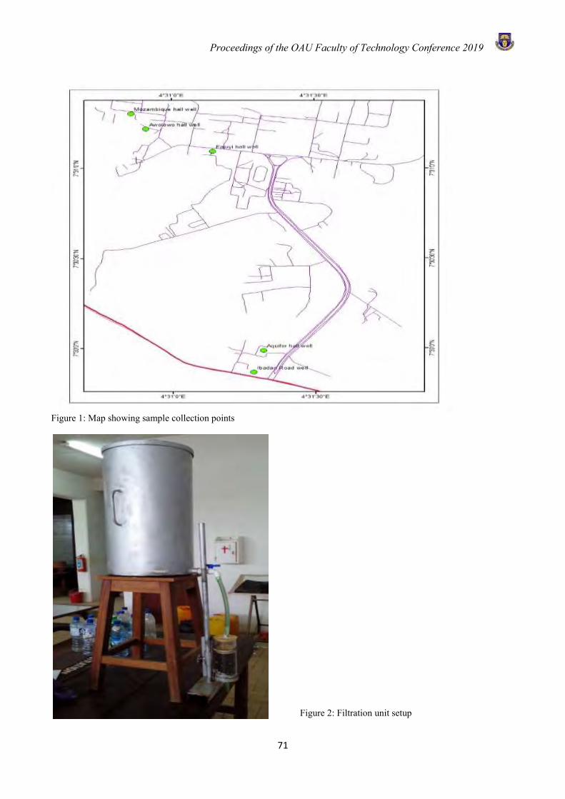
Proceedings of the OAU Faculty of Technology Conference 2019
71
Figure 1: Map showing sample collection points
Figure 2: Filtration unit setup
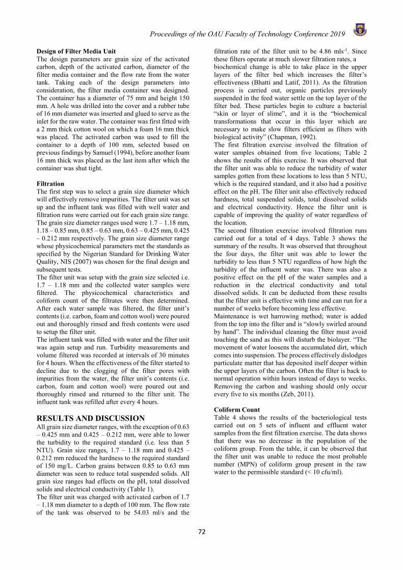
Proceedings of the OAU Faculty of Technology Conference 2019
72
Design of Filter Media Unit The design parameters are grain size of the activated carbon, depth of the activated carbon, diameter of the filter media container and the flow rate from the water tank. Taking each of the design parameters into consideration, the filter media container was designed. The container has a diameter of 75 mm and height 150 mm. A hole was drilled into the cover and a rubber tube of 16 mm diameter was inserted and glued to serve as the inlet for the raw water. The container was first fitted with a 2 mm thick cotton wool on which a foam 16 mm thick was placed. The activated carbon was used to fill the container to a depth of 100 mm, selected based on previous findings by Samuel (1994), before another foam 16 mm thick was placed as the last item after which the container was shut tight. Filtration The first step was to select a grain size diameter which will effectively remove impurities. The filter unit was set up and the influent tank was filled with well water and filtration runs were carried out for each grain size range. The grain size diameter ranges used were 1.7 – 1.18 mm, 1.18 – 0.85 mm, 0.85 – 0.63 mm, 0.63 – 0.425 mm, 0.425 – 0.212 mm respectively. The grain size diameter range whose physicochemical parameters met the standards as specified by the Nigerian Standard for Drinking Water Quality, NIS (2007) was chosen for the final design and subsequent tests. The filter unit was setup with the grain size selected i.e. 1.7 – 1.18 mm and the collected water samples were filtered. The physicochemical characteristics and coliform count of the filtrates were then determined. After each water sample was filtered, the filter unit’s contents (i.e. carbon, foam and cotton wool) were poured out and thoroughly rinsed and fresh contents were used to setup the filter unit. The influent tank was filled with water and the filter unit was again setup and run. Turbidity measurements and volume filtered was recorded at intervals of 30 minutes for 4 hours. When the effectiveness of the filter started to decline due to the clogging of the filter pores with impurities from the water, the filter unit’s contents (i.e. carbon, foam and cotton wool) were poured out and thoroughly rinsed and returned to the filter unit. The influent tank was refilled after every 4 hours. RESULTS AND DISCUSSION All grain size diameter ranges, with the exception of 0.63 – 0.425 mm and 0.425 – 0.212 mm, were able to lower the turbidity to the required standard (i.e. less than 5 NTU). Grain size ranges, 1.7 – 1.18 mm and 0.425 – 0.212 mm reduced the hardness to the required standard of 150 mg/L. Carbon grains between 0.85 to 0.63 mm diameter was seen to reduce total suspended solids. All grain size ranges had effects on the pH, total dissolved solids and electrical conductivity (Table 1). The filter unit was charged with activated carbon of 1.7 – 1.18 mm diameter to a depth of 100 mm. The flow rate of the tank was observed to be 54.03 ml/s and the
filtration rate of the filter unit to be 4.86 mls-1. Since these filters operate at much slower filtration rates, a biochemical change is able to take place in the upper layers of the filter bed which increases the filter’s effectiveness (Bhatti and Latif, 2011). As the filtration process is carried out, organic particles previously suspended in the feed water settle on the top layer of the filter bed. These particles begin to culture a bacterial “skin or layer of slime”, and it is the “biochemical transformations that occur in this layer which are necessary to make slow filters efficient as filters with biological activity” (Chapman, 1992). The first filtration exercise involved the filtration of water samples obtained from five locations; Table 2 shows the results of this exercise. It was observed that the filter unit was able to reduce the turbidity of water samples gotten from these locations to less than 5 NTU, which is the required standard, and it also had a positive effect on the pH. The filter unit also effectively reduced hardness, total suspended solids, total dissolved solids and electrical conductivity. Hence the filter unit is capable of improving the quality of water regardless of the location. The second filtration exercise involved filtration runs carried out for a total of 4 days. Table 3 shows the summary of the results. It was observed that throughout the four days, the filter unit was able to lower the turbidity to less than 5 NTU regardless of how high the turbidity of the influent water was. There was also a positive effect on the pH of the water samples and a reduction in the electrical conductivity and total dissolved solids. It can be deducted from these results that the filter unit is effective with time and can run for a number of weeks before becoming less effective. Maintenance is wet harrowing method; water is added from the top into the filter and is “slowly swirled around by hand”. The individual cleaning the filter must avoid touching the sand as this will disturb the biolayer. “The movement of water loosens the accumulated dirt, which comes into suspension. The process effectively dislodges particulate matter that has deposited itself deeper within the upper layers of the carbon. Often the filter is back to normal operation within hours instead of days to weeks. Removing the carbon and washing should only occur every five to six months (Zeb, 2011). Coliform Count Table 4 shows the results of the bacteriological tests carried out on 5 sets of influent and effluent water samples from the first filtration exercise. The data shows that there was no decrease in the population of the coliform group. From the table, it can be observed that the filter unit was unable to reduce the most probable number (MPN) of coliform group present in the raw water to the permissible standard (< 10 cfu/ml).
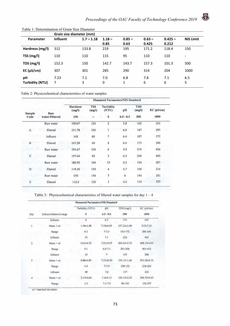
Proceedings of the OAU Faculty of Technology Conference 2019
73
Table 1: Determination of Grain Size Diameter Grain size diameter (mm)
Parameter Influent 1.7 – 1.18 1.18 – 0.85
0.85 – 0.63
0.63 – 0.425
0.425 – 0.212
NIS Limit
Hardness (mg/l) 312 133.8 219 195 171.2 118.4 150
TSS (mg/l) 110 110 115 95 110 110 -
TDS (mg/l) 152.3 150 142.7 143.7 157.3 101.3 500
EC (µS/cm) 307 301 285 290 314 204 1000
pH 7.23 7.1 7.0 6.8 7.8 7.1 6.5 Turbidity (NTU) 7 3 0 1 6 6 5
Table 2: Physicochemical characteristics of water samples
Table 3: Physicochemical characteristics of filtered water samples for day 1 – 4
Proceedings of the OAU Faculty of Technology Conference 2019
74
CONCLUSION The study concluded that the filter unit effectively lowered the turbidity and hardness to the permissible standard (5 NTU and 150 mg/L) for potable water. The filter unit also effectively reduced the electrical conductivity and total dissolved solids and was seen to have a positive effect on the pH. Activated carbon of 1.7 – 1.18 mm diameter was found to be the best in effectively improving the water quality and the filter unit is more effective with time. The designed household-scale filter was very efficient in removing the different turbidity levels to ≤ 5 NTU. REFERENCES Bhatti, M. T. and Latif, M. (2011). Assessment of water
quality of a river using an indexing approach during the low-flow season. Irrigation Drainage, 60: 103-114.
Butu, A.W. and Bichi, A. A. (2013). Assessment of some heavy elements in Galma dam, Zaria, Nigeria. International Journal of Development and Sustainability, 2(2): 686-696.
Chapman, D. (1992). Water Quality Assessments; A guide to the use of Biota, Sediments and Water in Environmental monitoring, UNESCO/ WHO/ UNEP.
Gleick, P. (2013). ‘Water in Crisis: A Guide to the Worlds’s Freshwater Resources’. Oxford: Oxford University Press.
Greenburg, R. (2005). ‘The Ocean Moon: Search for an Alien Biosphere’. Springer Praxis Books.
Jeje, J.O. and Oladepo, K.T (2014) Assessment of Heavy Metals of Boreholes and Hand Dug wells in Ife North Local Government Area of Osun State, Nigeria, International Journal of Science and Technology 3(4): 209-214.
Nigerian Industrial Standard (2007). ‘Nigerian Standard for Drinking Water Quality’ SON Governing Council, NIS 554:2007.
Ogedengbe, M.O., Oriaje, A.T. and Tella, A. (1985). Carbonisation and Activation of Palm Kernel Shells for Household Water Filters. Water International 10: 132-138.
Samuel, O.A. (1994). The Removal of Colour, Odour and Taste from Well Water – using Activated Carbon Prepared from Palm Kernel Shells and Cow bones. B.Sc. Thesis, Department of Civil Engineering, Obafemi Awolowo University, Ile-Ife, Nigeria.
WHO/UNICEF (2012). Progress on Sanitation and Drinking Water. 2012 Update. WHO/UNICEF. Geneva, Switzerland.
WHO/UNICEF (2015). Progress on Saniation and Drinking Water. 2015 Update and MDG Assessment. WHO/UNICEF. Geneva, Switzerland.
Zeb, B. S., Malik, A. H., Waseem, A. and Mahmood, Q. (2011). Water Quality Assessment of Siranriver, Pakistan. International Journal of Physical Sciences, 6(8): 7789- 7798.
Proceedings of the OAU Faculty of Technology Conference 2019
75
DISTRIBUTION SYSTEM VOLTAGE PROFILE IMPROVEMENT BASED ON NETWORK STRUCTURAL CHARACTERISTICS
S. O. Ayanlade*1 and O. A. Komolafe1 1 Electronic and Electrical Engineering Department Obafemi Awolowo University, Ile-Ife, Nigeria.
*Email of Corresponding Author: [email protected]
ABSTRACT Reactive power compensator placement is a method used to improve voltage profile in distribution systems. Inherent structural characteristic theory (ISCT) can determine the location of reactive power compensator using circuit law without running repetitive load flow. The objective of this paper is to present a fast method of determining the appropriate location of reactive power compensator. The method was applied to Imalefalafia 32-bus and IEEE 33-bus radial distribution networks and the results compared with the voltage stability index (VSI) and QV sensitivity methods. The results showed that the appropriate locations were buses 24 and 30 for Imalefalafia 32-bus and IEEE 33-bus, respectively. The minimum voltage magnitudes increased by 1.73 and 6.24% for Imalefalafia 32-bus and IEEE 33-bus, respectively after injection. The appropriate location selected by VSI and QV sensitivity methods were buses 22 and 23, respectively for Imalefalafia 32-bus and buses 18 and 30, respectively for IEEE 33-bus. The minimum voltage magnitudes increased by 1.41 and 2.14%, respectively and by 1.65 and 6.24%, respectively after injection. The computational time for ISCT were 0.002766 and 0.03635 s as compared with VSI which were 0.12973 and 0.238727 s, respectively and QV which were 0.009257 and 0.120055 s, respectively. In each case, the ISCT method was faster and improved the voltage profile better. Keywords: Inherent structural characteristic, voltage stability index, QV sensitivity, structural impact of load electrical attraction region. INTRODUCTION The distribution system network serves as a final link between the high voltage transmission system and the consumers. It is constructed with the aim of delivering electric power to the end users (Ighalo and Williams, 2012). Distribution networks suffer from poor voltage profile due to its inherent structural nature. They are considered as ill-conditioned networks because of their high resistance-to-reactance ratio, large number of nodes and untransposed conductors. Therefore, the node voltages are subjected to voltage fluctuations and if they are not quickly attended to, by taken appropriate steps, may result in voltage collapse. In power systems, it is required that the voltages at all the buses are within acceptable limits. To ensure that voltage profiles are acceptable in distribution systems, different standards have been recommended. For instance, the power regulatory body in Nigeria has required that voltage fluctuations in power systems must be maintained within ±5% of the nominal voltage. One of the popularly used techniques to improve voltage profiles in power systems is the introduction of reactive power compensators. For optimal benefit, it is required that reactive power compensators be properly sized and located. Studies show that improper selection of size and location of reactive power compensators leads to poor voltage profile improvement (Kim, 2001a, b; Acharya et al., 2006; Atwa et al., 2010).
Notable works have been done in this area of research using different methods to determine the optimal locations of reactive power compensators such as particle swarm optimization method (Reddy et al., 2012), genetic algorithm method (Kotb et al., 2010; Yadav and Srivastava, 2015), voltage stability index method (Arvindhababu and Mohan, 2009; Thishya and Balamurugan, 2017; Eminoglu and Hocaoglu, 2007), QV sensitivity method (Wang and Nehrir, 2004; Mithulananthan and Hien, 2013; Injeti and Kumar, 2011), fuzzy logic method etc. These solution approaches determine buses where reactive power compensators could best be placed. However, these existing methods usually involve the loading conditions that require performing time-consuming and repetitive power-flow equations. This paper presents a less computationally expensive method, which uses circuit theory to obtain the appropriate reactive power compensators’ location in distribution systems to improve the network voltage profile. Inherent Structural Characteristic Theory The inherent structural characteristics theory of suggests that the problem of power systems could be solved by the consideration of the interconnections of the components and the values of their impedances (Sikiru et al., 2013). This theory is dependent on the structural relationship between the voltages at the network buses and the currents passing in the network links (Carpinelli et al., 1998).
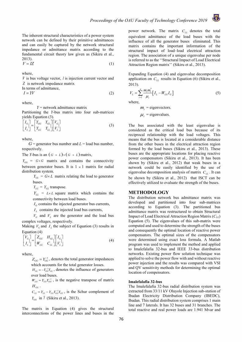
Proceedings of the OAU Faculty of Technology Conference 2019
76
The inherent structural characteristics of a power system network can be defined by their primitive admittances and can easily be captured by the network structural impedance or admittance matrix according to the fundamental circuit theory law given as (Sikiru et al., 2013). V IZ= (1) where, V is bus voltage vector, I is injection current vector and Z is network impedance matrix In terms of admittance, I YV= (2)
where,
Y = network admittance matrix Partitioning the Y-bus matrix into four sub-matrices yields Equation (3).
GG GLG G
LG LLL L
Y YI VY YI V
=
(3)
where,
G = generator bus number and L = load bus number, respectively. The Y-bus is an ( ) ( ) G L G L+ + matrix,
GGY = G G matrix and contains the connectivity between generator buses. It is 1 1 matrix for radial distribution system.
GLY = G L matrix relating the load to generator buses.
LGY = GLY transpose.
LLY = L L square matrix which contains the connectivity between load buses.
GI contains the injected generator bus currents,
LI contains the injected load bus currents,
GV and LV are the generator and the load bus complex voltages, respectively. Making GV and LI the subject of Equation (3) results in Equation (4)
GG GLG G
LG LLL L
Z HV IW CI V
=
(4)
where,
1GG GGZ Y −= , denotes the total generator impedances
which accounts for the total generator losses. 1
GL GG GLH Y Y−= − , denotes the influence of generators over load buses.
1LG LG GGW Y Y −= , is the negative transpose of matrix
GLH . 1
LL LL LG GG GLC Y Y Y Y−= − , is the Schur complement of
GGY in Y (Sikiru et al., 2013). The matrix in Equation (4) gives the structural interconnections of the power lines and buses in the
power network. The matrix LLC denotes the total equivalent admittance of the load buses with the influence of all the generator buses eliminated. This matrix contains the important information of the structural impact of load–load electrical attraction region. The association of a unique eigenvalue per node is referred to as the ‘‘Structural Impact of Load Electrical Attraction Region matrix’’ (Sikiru et al., 2013). Expanding Equation (4) and eigenvalue decomposition application on LLC results in Equation (6) (Sikiru et al., 2013).
*
1
ni i
L L LG Gi i
m mV I W I
=
= − (5)
where,
im = eigenvectors.
i = eigenvalues. The bus associated with the least eigenvalue is considered as the critical load bus because of its reciprocal relationship with the load voltages. This means that the bus is located at a considerable distance from the other buses in the electrical attraction region formed by the load buses (Sikiru et al., 2013). These buses are the appropriate locations for placing reactive power compensators (Sikiru et al., 2013). It has been shown by (Sikiru et al., 2012) that weak buses in a network could be easily identified by the use of eigenvalue decomposition analysis of matrix LLC . It can be shown by (Sikiru et al., 2012) that ISCT can be effectively utilized to evaluate the strength of the buses. METHODOLOGY The distribution network bus admittance matrix was developed and partitioned into four sub-matrices according to Equation (3). The partitioned bus admittance matrix was restructured to obtain Structural Impact of Load Electrical Attraction Region Matrix (CLL) Equation (5). The eigenvalues of this sub-matrix were computed and used to determine the strength of the buses and consequently the optimal location of reactive power compensators. The optimal sizes of the compensators were determined using exact loss formula. A Matlab program was used to implement the method and applied to Imalefalafia 32-bus and IEEE 33-bus distribution networks. Existing power flow solution technique was applied to solve the power flow with and without reactive power injection and the results was compared with VSI and QV sensitivity methods for determining the optimal location of compensators. Imalefalafia 32-bus The Imalefalafia 32-bus radial distribution system was extracted from 33/11 kV Oluyole Injection sub-station of Ibadan Electricity Distribution Company (IBEDC), Ibadan. This radial distribution system comprises 1 main line and 7 laterals. It has 32 buses and 31 branches. The total reactive and real power loads are 1.941 Mvar and
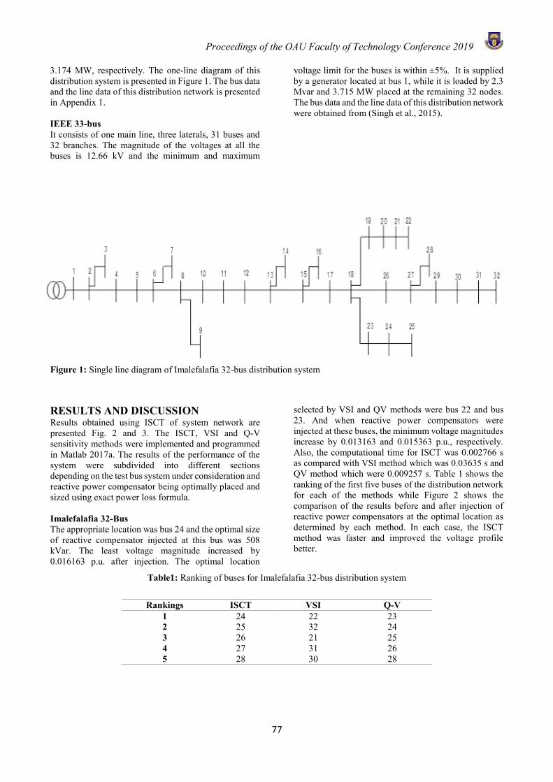
Proceedings of the OAU Faculty of Technology Conference 2019
77
3.174 MW, respectively. The one-line diagram of this distribution system is presented in Figure 1. The bus data and the line data of this distribution network is presented in Appendix 1. IEEE 33-bus It consists of one main line, three laterals, 31 buses and 32 branches. The magnitude of the voltages at all the buses is 12.66 kV and the minimum and maximum
voltage limit for the buses is within ±5%. It is supplied by a generator located at bus 1, while it is loaded by 2.3 Mvar and 3.715 MW placed at the remaining 32 nodes. The bus data and the line data of this distribution network were obtained from (Singh et al., 2015).
Figure 1: Single line diagram of Imalefalafia 32-bus distribution system
RESULTS AND DISCUSSION Results obtained using ISCT of system network are presented Fig. 2 and 3. The ISCT, VSI and Q-V sensitivity methods were implemented and programmed in Matlab 2017a. The results of the performance of the system were subdivided into different sections depending on the test bus system under consideration and reactive power compensator being optimally placed and sized using exact power loss formula. Imalefalafia 32-Bus The appropriate location was bus 24 and the optimal size of reactive compensator injected at this bus was 508 kVar. The least voltage magnitude increased by 0.016163 p.u. after injection. The optimal location
selected by VSI and QV methods were bus 22 and bus 23. And when reactive power compensators were injected at these buses, the minimum voltage magnitudes increase by 0.013163 and 0.015363 p.u., respectively. Also, the computational time for ISCT was 0.002766 s as compared with VSI method which was 0.03635 s and QV method which were 0.009257 s. Table 1 shows the ranking of the first five buses of the distribution network for each of the methods while Figure 2 shows the comparison of the results before and after injection of reactive power compensators at the optimal location as determined by each method. In each case, the ISCT method was faster and improved the voltage profile better.
Table1: Ranking of buses for Imalefalafia 32-bus distribution system
Rankings ISCT VSI Q-V
1 2 3 4 5
24 25 26 27 28
22 32 21 31 30
23 24 25 26 28
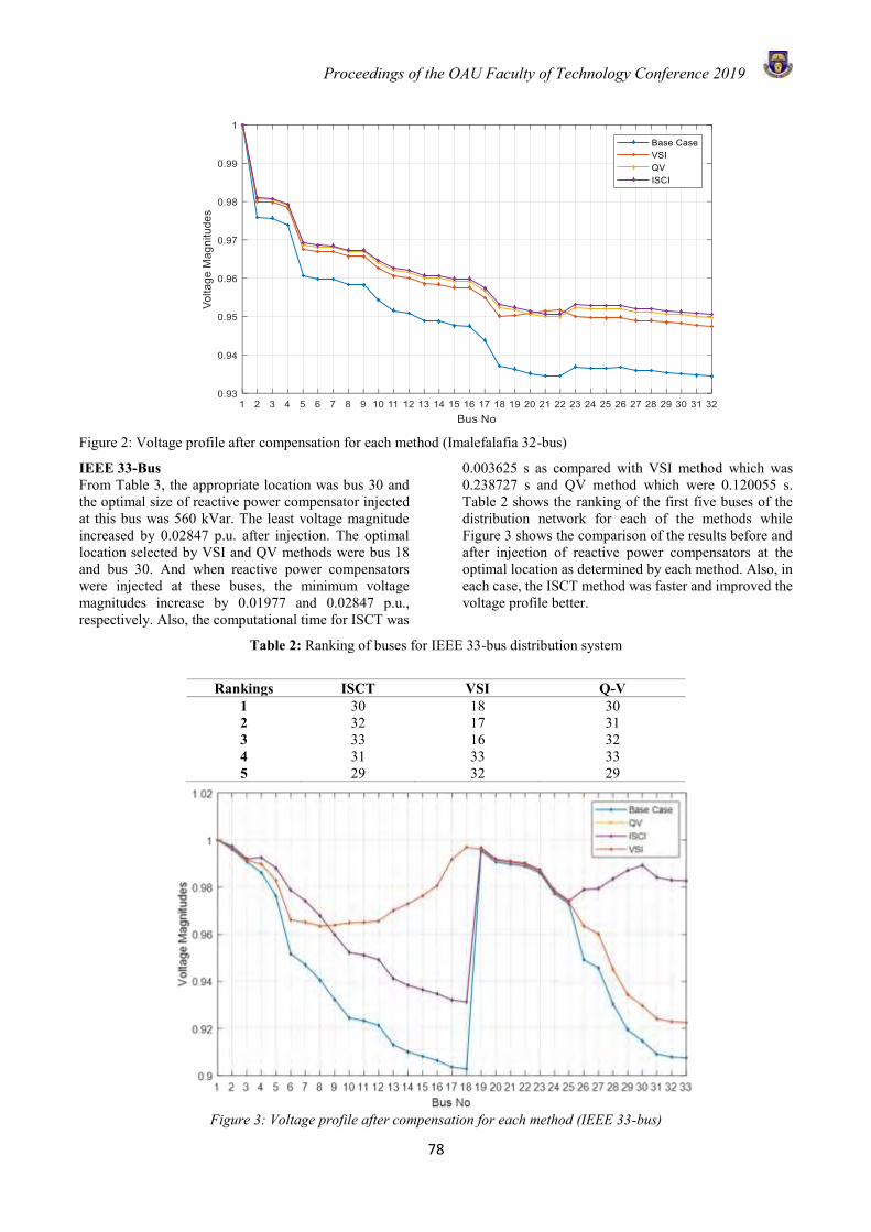
Proceedings of the OAU Faculty of Technology Conference 2019
78
Figure 2: Voltage profile after compensation for each method (Imalefalafia 32-bus)
IEEE 33-Bus From Table 3, the appropriate location was bus 30 and the optimal size of reactive power compensator injected at this bus was 560 kVar. The least voltage magnitude increased by 0.02847 p.u. after injection. The optimal location selected by VSI and QV methods were bus 18 and bus 30. And when reactive power compensators were injected at these buses, the minimum voltage magnitudes increase by 0.01977 and 0.02847 p.u., respectively. Also, the computational time for ISCT was
0.003625 s as compared with VSI method which was 0.238727 s and QV method which were 0.120055 s. Table 2 shows the ranking of the first five buses of the distribution network for each of the methods while Figure 3 shows the comparison of the results before and after injection of reactive power compensators at the optimal location as determined by each method. Also, in each case, the ISCT method was faster and improved the voltage profile better.
Table 2: Ranking of buses for IEEE 33-bus distribution system
Rankings ISCT VSI Q-V
1 2 3 4 5
30 32 33 31 29
18 17 16 33 32
30 31 32 33 29
Figure 3: Voltage profile after compensation for each method (IEEE 33-bus)
Proceedings of the OAU Faculty of Technology Conference 2019
79
CONCLUSION This paper showed the capability of improved voltage profile achievable using the approach of circuit theory applied to radial distribution system networks. The appropriate locations of reactive compensators were determined from the use of eigenvalue decomposition of a sub-matrix of the Y-bus. The study concluded that the ISCT method is more effective for determining the reactive power compensator location in radial distribution networks for improving network voltage profiles. REFERENCES Acharya, N., Mahat, P., and Mithulananthan, N., An
Analytical Approach for DG Allocation in Primary Distribution Network. Int. J. Electr. Power Energy Syst., 28(10):669–678, 2006.
Arvindhababu, P., and Mohan, G., Optimal Capacitor Placement for Voltage Stability Enhancement in Distribution Systems. ARPN Journal of Engineering and Applied Sciences, 4(2):88–92, 2009.
Atwa, Y., El-Saadany, E., Salama, M., and Seethapathy, R., Optimal Renewable Resources Mix for Distribution System Energy Loss Minimization. IEEE Transaction on Power System, 25(2):360–370, 2010.
Carpinelli, G., Russo, A., Russo, M., and Verde, P., Inherent Structure Theory of Networks and Power System Harmonics. IEEE Proceedings – Generation, Transmission and Distribution, 2(1):123–132, 1998.
Eminoglu, U., and Hocaoglu, M. H., A Voltage Stability Index for Radial Distribution Networks. 42nd International Universities Power Engineering Conference, Pp. 408–413, 2007.
Ighalo, G. I., and Williams, A. A., Simulating Power Distribution Network in Nigeria –The Ikpoba-Hill District Network as A Case Study. International Journal of Scientific & Technology Research, 1(9):1–8, 2012.
Injeti, S. K., and Kumar, N. P., Optimal Planning of Distributed Generation for Improved Voltage Stability and Loss Reduction.” International Journal of Computer Applications, 15(1):40–46, 2011.
Kim, T. E., Voltage Regulation Coordination of Distributed Generation System in Distribution System. IEEE Transaction on Power Delivery, 6(3):1100–1117, 2001a.
Kim, T. E., A Method for Determining the Introduction Limit of Distributed Generation System in Distribution System. IEEE Transaction on Power Delivery, 4(2):100–117, 2001b.
Kotb, M. F., Shebl, K. M., El Khazendar, M., and El Husseiny, A., Genetic Algorithm for Optimum Siting and Sizing of Distributed Generation. Proc. 14th Int. Middle East Power Systems Conference, Pp. 433–440, 2010.
Mithulananthan, N., and Hien, N. C., Location and Sizing of Distributed Generation Units for Loadability Enhancement in Primary Feeder. IEEE systems Journal, 7(4):1–10, 2013.
Reddy, S. C., Prasad, P. V. N., and Laxmi, A. J., Power Quality and Reliability Improvement of Distribution System by Optimal Number, Location and Size of DGs Using Particle Swarm Optimization. 7th IEEE International Conference on Industrial and Information Systems (ICIIS), Pp. 0–6, 2012.
Sikiru, T. H., Jimoh, A. A., and Agee, J. T., Inherent structural characteristic indices of power system networks. International Journal of Electrical Power and Energy Systems, 47(1):218–224, 2013.
Sikiru, T. H., Jimoh, A. A., Hamam, Y., Agee, J. T., and Ceschi, R., Relationship Between Generator Affinity and Voltage Profile Improvement. IEEE 10th International Power and Energy Conference (IPEC), Pp. 451- 454, 2012.
Singh, N., Ghosh, S., and Murari, K., Optimal Sizing and Placement of DG in a Radial Distribution Network using Sensitivity based Methods. International Electrical Engineering Journal (IEEJ), 6(1):1727–1734, 2015.
Thishya, V. U., and Balamurugan, K., Optimal Placement of Distributed Generation with SVC for Power Loss Reduction in Distributed System. ARPN Journal of Engineering and Applied Sciences, 12(17):4895–4901, 2017.
Wang, C., and Nehrir, H., Analytical Approaches for Optimal Placement of Distributed Generation Sources in Power System. IEEE Transaction on Power Systems, 19(4):2068–2076, 2004.
Yadav, P. S., and Srivastava, L., Optimal Location of Combined DG and Capacitor for Real Power Loss Minimization in Distribution Networks. International Journal of Electrical and Electronics Engineers, 7(1):222–233, 2015.
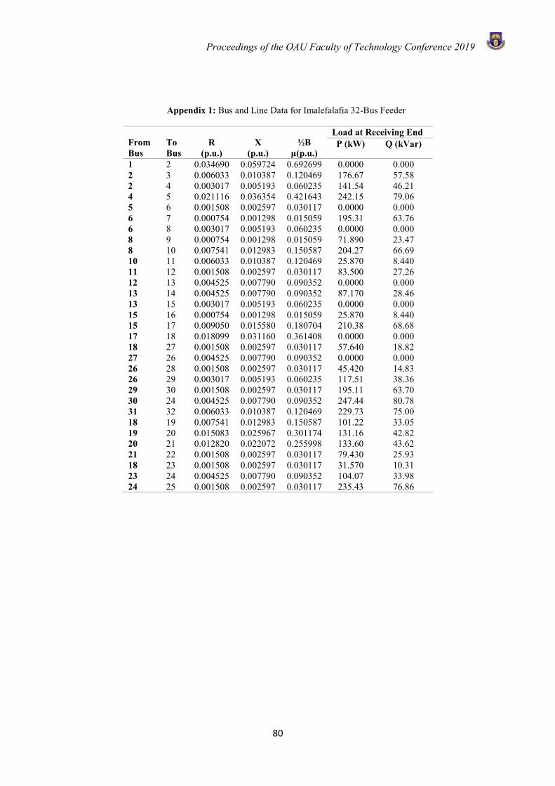
Proceedings of the OAU Faculty of Technology Conference 2019
80
Appendix 1: Bus and Line Data for Imalefalafia 32-Bus Feeder
From Bus
To Bus
R (p.u.)
X (p.u.)
½B µ(p.u.)
Load at Receiving End P (kW) Q (kVar)
1 2 2 4 5 6 6 8 8 10 11 12 13 13 15 15 17 18 27 26 26 29 30 31 18 19 20 21 18 23 24
2 3 4 5 6 7 8 9 10 11 12 13 14 15 16 17 18 27 26 28 29 30 24 32 19 20 21 22 23 24 25
0.034690 0.006033 0.003017 0.021116 0.001508 0.000754 0.003017 0.000754 0.007541 0.006033 0.001508 0.004525 0.004525 0.003017 0.000754 0.009050 0.018099 0.001508 0.004525 0.001508 0.003017 0.001508 0.004525 0.006033 0.007541 0.015083 0.012820 0.001508 0.001508 0.004525 0.001508
0.059724 0.010387 0.005193 0.036354 0.002597 0.001298 0.005193 0.001298 0.012983 0.010387 0.002597 0.007790 0.007790 0.005193 0.001298 0.015580 0.031160 0.002597 0.007790 0.002597 0.005193 0.002597 0.007790 0.010387 0.012983 0.025967 0.022072 0.002597 0.002597 0.007790 0.002597
0.692699 0.120469 0.060235 0.421643 0.030117 0.015059 0.060235 0.015059 0.150587 0.120469 0.030117 0.090352 0.090352 0.060235 0.015059 0.180704 0.361408 0.030117 0.090352 0.030117 0.060235 0.030117 0.090352 0.120469 0.150587 0.301174 0.255998 0.030117 0.030117 0.090352 0.030117
0.0000 176.67 141.54 242.15 0.0000 195.31 0.0000 71.890 204.27 25.870 83.500 0.0000 87.170 0.0000 25.870 210.38 0.0000 57.640 0.0000 45.420 117.51 195.11 247.44 229.73 101.22 131.16 133.60 79.430 31.570 104.07 235.43
0.000 57.58 46.21 79.06 0.000 63.76 0.000 23.47 66.69 8.440 27.26 0.000 28.46 0.000 8.440 68.68 0.000 18.82 0.000 14.83 38.36 63.70 80.78 75.00 33.05 42.82 43.62 25.93 10.31 33.98 76.86
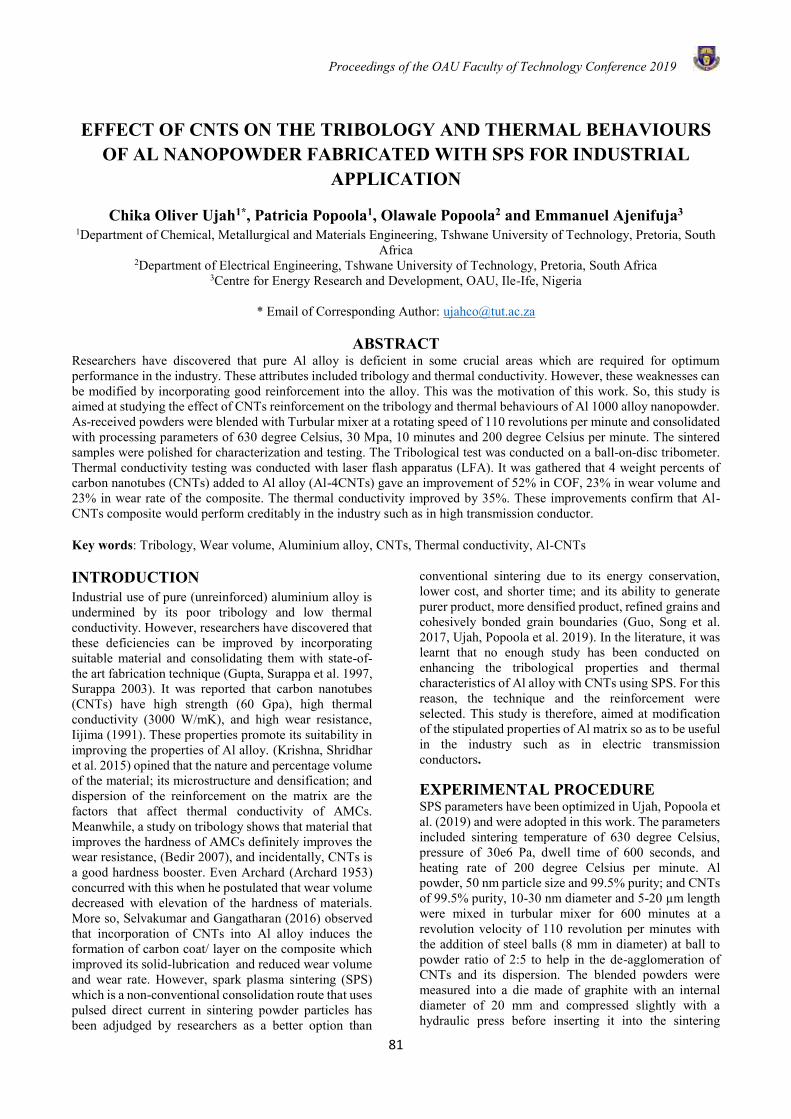
Proceedings of the OAU Faculty of Technology Conference 2019
81
EFFECT OF CNTS ON THE TRIBOLOGY AND THERMAL BEHAVIOURS OF AL NANOPOWDER FABRICATED WITH SPS FOR INDUSTRIAL
APPLICATION
Chika Oliver Ujah1*, Patricia Popoola1, Olawale Popoola2 and Emmanuel Ajenifuja3 1Department of Chemical, Metallurgical and Materials Engineering, Tshwane University of Technology, Pretoria, South
Africa 2Department of Electrical Engineering, Tshwane University of Technology, Pretoria, South Africa
3Centre for Energy Research and Development, OAU, Ile-Ife, Nigeria
* Email of Corresponding Author: [email protected]
ABSTRACT Researchers have discovered that pure Al alloy is deficient in some crucial areas which are required for optimum performance in the industry. These attributes included tribology and thermal conductivity. However, these weaknesses can be modified by incorporating good reinforcement into the alloy. This was the motivation of this work. So, this study is aimed at studying the effect of CNTs reinforcement on the tribology and thermal behaviours of Al 1000 alloy nanopowder. As-received powders were blended with Turbular mixer at a rotating speed of 110 revolutions per minute and consolidated with processing parameters of 630 degree Celsius, 30 Mpa, 10 minutes and 200 degree Celsius per minute. The sintered samples were polished for characterization and testing. The Tribological test was conducted on a ball-on-disc tribometer. Thermal conductivity testing was conducted with laser flash apparatus (LFA). It was gathered that 4 weight percents of carbon nanotubes (CNTs) added to Al alloy (Al-4CNTs) gave an improvement of 52% in COF, 23% in wear volume and 23% in wear rate of the composite. The thermal conductivity improved by 35%. These improvements confirm that Al-CNTs composite would perform creditably in the industry such as in high transmission conductor. Key words: Tribology, Wear volume, Aluminium alloy, CNTs, Thermal conductivity, Al-CNTs
INTRODUCTION Industrial use of pure (unreinforced) aluminium alloy is undermined by its poor tribology and low thermal conductivity. However, researchers have discovered that these deficiencies can be improved by incorporating suitable material and consolidating them with state-of-the art fabrication technique (Gupta, Surappa et al. 1997, Surappa 2003). It was reported that carbon nanotubes (CNTs) have high strength (60 Gpa), high thermal conductivity (3000 W/mK), and high wear resistance, Iijima (1991). These properties promote its suitability in improving the properties of Al alloy. (Krishna, Shridhar et al. 2015) opined that the nature and percentage volume of the material; its microstructure and densification; and dispersion of the reinforcement on the matrix are the factors that affect thermal conductivity of AMCs. Meanwhile, a study on tribology shows that material that improves the hardness of AMCs definitely improves the wear resistance, (Bedir 2007), and incidentally, CNTs is a good hardness booster. Even Archard (Archard 1953) concurred with this when he postulated that wear volume decreased with elevation of the hardness of materials. More so, Selvakumar and Gangatharan (2016) observed that incorporation of CNTs into Al alloy induces the formation of carbon coat/ layer on the composite which improved its solid-lubrication and reduced wear volume and wear rate. However, spark plasma sintering (SPS) which is a non-conventional consolidation route that uses pulsed direct current in sintering powder particles has been adjudged by researchers as a better option than
conventional sintering due to its energy conservation, lower cost, and shorter time; and its ability to generate purer product, more densified product, refined grains and cohesively bonded grain boundaries (Guo, Song et al. 2017, Ujah, Popoola et al. 2019). In the literature, it was learnt that no enough study has been conducted on enhancing the tribological properties and thermal characteristics of Al alloy with CNTs using SPS. For this reason, the technique and the reinforcement were selected. This study is therefore, aimed at modification of the stipulated properties of Al matrix so as to be useful in the industry such as in electric transmission conductors.
EXPERIMENTAL PROCEDURE SPS parameters have been optimized in Ujah, Popoola et al. (2019) and were adopted in this work. The parameters included sintering temperature of 630 degree Celsius, pressure of 30e6 Pa, dwell time of 600 seconds, and heating rate of 200 degree Celsius per minute. Al powder, 50 nm particle size and 99.5% purity; and CNTs of 99.5% purity, 10-30 nm diameter and 5-20 µm length were mixed in turbular mixer for 600 minutes at a revolution velocity of 110 revolution per minutes with the addition of steel balls (8 mm in diameter) at ball to powder ratio of 2:5 to help in the de-agglomeration of CNTs and its dispersion. The blended powders were measured into a die made of graphite with an internal diameter of 20 mm and compressed slightly with a hydraulic press before inserting it into the sintering
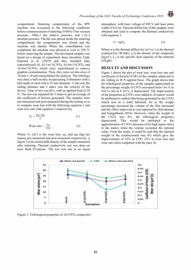
Proceedings of the OAU Faculty of Technology Conference 2019
82
compartment. Sintering compartment of the SPS machine was evacuated to the following conditions before commencement of sintering: 0.605e-3 bar vacuum pressure, -500e-3 bar relative pressure, and 1.2e-3 absolute pressure. The die was placed inside the sintering compartment; the compartment was closed and the machine was started. When the consolidation was completed, the machine was allowed to cool to 250 before removing the sample. The developed samples was based on a design of experiment done elsewhere Ujah, Popoola et al. (2019) and they included pure (unreinforced) Al, Al-1wt.%CNTs, Al-4wt.%CNTs, and Al-8wt.%CNTs which were sand-blasted to remove graphite contamination. Then, they were cut into sizes of 10 mm x 10 mm and polished for analysis. The tribology was done a ball-on-disc reciprocating Tribometer with a ball made of steel with 6.35 mm diameter. 5 mm was the sliding distance and 3 mm/s was the velocity of the device. Time of test was 60 s, with an applied load of 20 N. The test was repeated for 3 times to get an average of the coefficient of friction generated. The samples were pre-measured and post-measured during the testing so as to compute wear loss with the following equation 1 and wear loss rate with equation 2 respectively.
VL = 𝑚𝐴−𝑚𝐵
𝜌 (1)
Wear rate = 𝑉𝐿
𝑡𝑖𝑚𝑒 (2)
Where VL (m3) is the wear loss, mA and mB (kg) are masses pre-measured and post-measured respectively, ρ (kg/m3) is the actual bulk density of the sample measured after sintering. Thermal conductivity test was done on laser flash 82 nalyser. The test was run in an argon
atmosphere, with laser voltage of 450 V and laser pulse width of 0.8 ms. Thermal diffusivity of the samples were obtained and used to compute the thermal conductivity with equation 2.
Λ = αρCp (3)
Where α is the thermal diffusivity (m2/s), λ is the thermal conductivity (W/mK), ρ is the density of the composite (kg/m3), Cp is the specific heat capacity of the material (J/KgK).
RESULTS AND DISCUSSION Figure 1 shows the plot of wear loss, wear loss rate and coefficient of friction (COF) of the samples subjected to dry sliding at 20 N applied force. The graph shows that the tribological properties of the samples appreciated as the percentage weight of CNTs increased from 1wt.% to 4wt.%, but at 8 wt.%, it depreciated. The improvement of the properties as CNTs were added to Al matrix would be attributed to carbon film being generated by the CNTs which acts as a solid lubricant. So as the weight percentage increased the volume of the film increased and the effect improved as was reported by (Selvakumar and Gangatharan 2016). However, when the weight of the CNTs was 8%, the tribological properties depreciated. This would be attributed to the agglomeration of CNTs (because of its high aspect ratio) in the matrix when the volume exceeded the optimal value. From the study, it could be said that the optimal weight of the reinforcement was 4% which gave the improvements of 52% in COF, 23% in wear loss and wear rate when compared with the pure Al.
Figure 1: Tribological properties of Al-CNTs composites
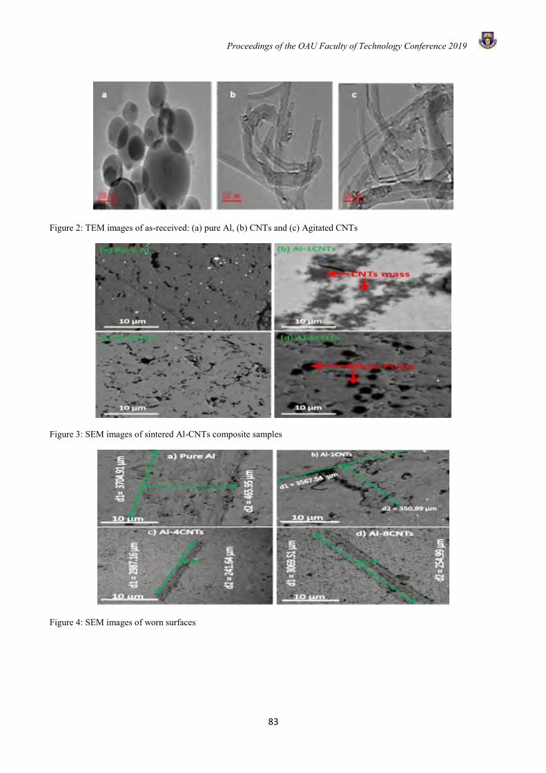
Proceedings of the OAU Faculty of Technology Conference 2019
83
Figure 2: TEM images of as-received: (a) pure Al, (b) CNTs and (c) Agitated CNTs
Figure 3: SEM images of sintered Al-CNTs composite samples
Figure 4: SEM images of worn surfaces
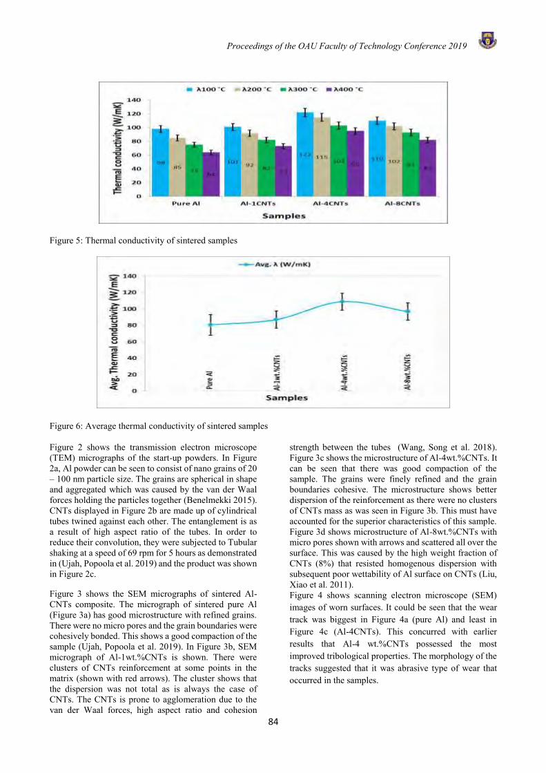
Proceedings of the OAU Faculty of Technology Conference 2019
84
Figure 5: Thermal conductivity of sintered samples
Figure 6: Average thermal conductivity of sintered samples
Figure 2 shows the transmission electron microscope (TEM) micrographs of the start-up powders. In Figure 2a, Al powder can be seen to consist of nano grains of 20 – 100 nm particle size. The grains are spherical in shape and aggregated which was caused by the van der Waal forces holding the particles together (Benelmekki 2015). CNTs displayed in Figure 2b are made up of cylindrical tubes twined against each other. The entanglement is as a result of high aspect ratio of the tubes. In order to reduce their convolution, they were subjected to Tubular shaking at a speed of 69 rpm for 5 hours as demonstrated in (Ujah, Popoola et al. 2019) and the product was shown in Figure 2c.
Figure 3 shows the SEM micrographs of sintered Al-CNTs composite. The micrograph of sintered pure Al (Figure 3a) has good microstructure with refined grains. There were no micro pores and the grain boundaries were cohesively bonded. This shows a good compaction of the sample (Ujah, Popoola et al. 2019). In Figure 3b, SEM micrograph of Al-1wt.%CNTs is shown. There were clusters of CNTs reinforcement at some points in the matrix (shown with red arrows). The cluster shows that the dispersion was not total as is always the case of CNTs. The CNTs is prone to agglomeration due to the van der Waal forces, high aspect ratio and cohesion
strength between the tubes (Wang, Song et al. 2018). Figure 3c shows the microstructure of Al-4wt.%CNTs. It can be seen that there was good compaction of the sample. The grains were finely refined and the grain boundaries cohesive. The microstructure shows better dispersion of the reinforcement as there were no clusters of CNTs mass as was seen in Figure 3b. This must have accounted for the superior characteristics of this sample. Figure 3d shows microstructure of Al-8wt.%CNTs with micro pores shown with arrows and scattered all over the surface. This was caused by the high weight fraction of CNTs (8%) that resisted homogenous dispersion with subsequent poor wettability of Al surface on CNTs (Liu, Xiao et al. 2011). Figure 4 shows scanning electron microscope (SEM) images of worn surfaces. It could be seen that the wear track was biggest in Figure 4a (pure Al) and least in Figure 4c (Al-4CNTs). This concurred with earlier results that Al-4 wt.%CNTs possessed the most improved tribological properties. The morphology of the tracks suggested that it was abrasive type of wear that occurred in the samples.
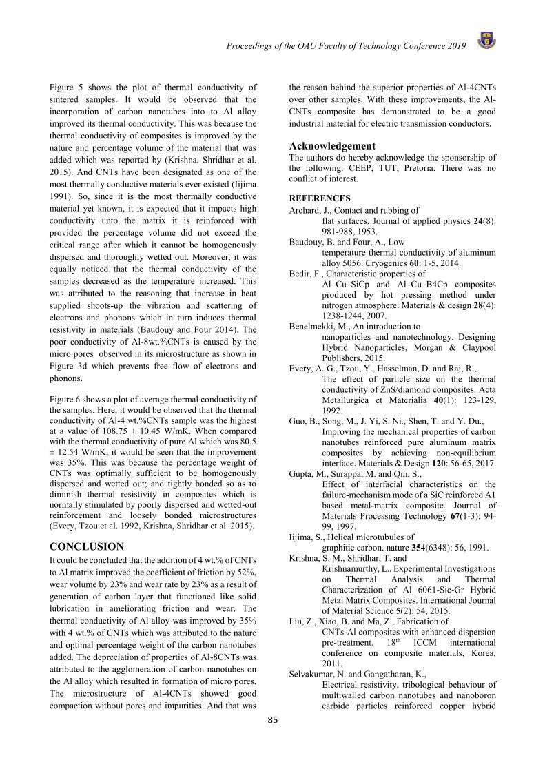
Proceedings of the OAU Faculty of Technology Conference 2019
85
Figure 5 shows the plot of thermal conductivity of sintered samples. It would be observed that the incorporation of carbon nanotubes into to Al alloy improved its thermal conductivity. This was because the thermal conductivity of composites is improved by the nature and percentage volume of the material that was added which was reported by (Krishna, Shridhar et al. 2015). And CNTs have been designated as one of the most thermally conductive materials ever existed (Iijima 1991). So, since it is the most thermally conductive material yet known, it is expected that it impacts high conductivity unto the matrix it is reinforced with provided the percentage volume did not exceed the critical range after which it cannot be homogenously dispersed and thoroughly wetted out. Moreover, it was equally noticed that the thermal conductivity of the samples decreased as the temperature increased. This was attributed to the reasoning that increase in heat supplied shoots-up the vibration and scattering of electrons and phonons which in turn induces thermal resistivity in materials (Baudouy and Four 2014). The poor conductivity of Al-8wt.%CNTs is caused by the micro pores observed in its microstructure as shown in Figure 3d which prevents free flow of electrons and phonons.
Figure 6 shows a plot of average thermal conductivity of the samples. Here, it would be observed that the thermal conductivity of Al-4 wt.%CNTs sample was the highest at a value of 108.75 ± 10.45 W/mK. When compared with the thermal conductivity of pure Al which was 80.5 ± 12.54 W/mK, it would be seen that the improvement was 35%. This was because the percentage weight of CNTs was optimally sufficient to be homogenously dispersed and wetted out; and tightly bonded so as to diminish thermal resistivity in composites which is normally stimulated by poorly dispersed and wetted-out reinforcement and loosely bonded microstructures (Every, Tzou et al. 1992, Krishna, Shridhar et al. 2015).
CONCLUSION It could be concluded that the addition of 4 wt.% of CNTs to Al matrix improved the coefficient of friction by 52%, wear volume by 23% and wear rate by 23% as a result of generation of carbon layer that functioned like solid lubrication in ameliorating friction and wear. The thermal conductivity of Al alloy was improved by 35% with 4 wt.% of CNTs which was attributed to the nature and optimal percentage weight of the carbon nanotubes added. The depreciation of properties of Al-8CNTs was attributed to the agglomeration of carbon nanotubes on the Al alloy which resulted in formation of micro pores. The microstructure of Al-4CNTs showed good compaction without pores and impurities. And that was
the reason behind the superior properties of Al-4CNTs over other samples. With these improvements, the Al-CNTs composite has demonstrated to be a good industrial material for electric transmission conductors.
Acknowledgement The authors do hereby acknowledge the sponsorship of the following: CEEP, TUT, Pretoria. There was no conflict of interest.
REFERENCES Archard, J., Contact and rubbing of
flat surfaces, Journal of applied physics 24(8): 981-988, 1953.
Baudouy, B. and Four, A., Low temperature thermal conductivity of aluminum alloy 5056. Cryogenics 60: 1-5, 2014.
Bedir, F., Characteristic properties of Al–Cu–SiCp and Al–Cu–B4Cp composites produced by hot pressing method under nitrogen atmosphere. Materials & design 28(4): 1238-1244, 2007.
Benelmekki, M., An introduction to nanoparticles and nanotechnology. Designing Hybrid Nanoparticles, Morgan & Claypool Publishers, 2015.
Every, A. G., Tzou, Y., Hasselman, D. and Raj, R., The effect of particle size on the thermal conductivity of ZnS/diamond composites. Acta Metallurgica et Materialia 40(1): 123-129, 1992.
Guo, B., Song, M., J. Yi, S. Ni., Shen, T. and Y. Du., Improving the mechanical properties of carbon nanotubes reinforced pure aluminum matrix composites by achieving non-equilibrium interface. Materials & Design 120: 56-65, 2017.
Gupta, M., Surappa, M. and Qin. S., Effect of interfacial characteristics on the failure-mechanism mode of a SiC reinforced A1 based metal-matrix composite. Journal of Materials Processing Technology 67(1-3): 94-99, 1997.
Iijima, S., Helical microtubules of graphitic carbon. nature 354(6348): 56, 1991.
Krishna, S. M., Shridhar, T. and Krishnamurthy, L., Experimental Investigations on Thermal Analysis and Thermal Characterization of Al 6061-Sic-Gr Hybrid Metal Matrix Composites. International Journal of Material Science 5(2): 54, 2015.
Liu, Z., Xiao, B. and Ma, Z., Fabrication of CNTs-Al composites with enhanced dispersion pre-treatment. 18th ICCM international conference on composite materials, Korea, 2011.
Selvakumar, N. and Gangatharan, K., Electrical resistivity, tribological behaviour of multiwalled carbon nanotubes and nanoboron carbide particles reinforced copper hybrid

Proceedings of the OAU Faculty of Technology Conference 2019
86
composites for pantograph application. Advances in Materials Science and Engineering, 2016.
Surappa, M., Aluminium matrix composites: Challenges and opportunities. Sadhana 28(1-2): 319-334, 2003.
Ujah, C. O.,Popoola, A. P., Popoola, O. M. and Aigbodion, V. S., Enhanced tribology, thermal and electrical properties of Al-CNT composite processed via spark plasma sintering for transmission conductor. Journal of Materials Science: 1-10, 2019.
Ujah, C. O.,Popoola, A. P., Popoola, O. M. and Aigbodion, V. S., Optimisation of spark plasma sintering parameters of Al-CNTs-Nb nano-composite using Taguchi Design of Experiment. The
International Journal of Advanced Manufacturing Technology 100(5-8): 1563-1573, 2019.
Ujah, C. O.,Popoola, A. P., Popoola, O. M. and Aigbodion, V. S., Enhanced mechanical, electrical and corrosion characteristics of Al-CNTs-Nb composite processed via spark plasma sintering for conductor core. Journal of Composite Materials: 0021998319848055, 2019.
Wang, T., Song, B., Qiao, K., Huang Y. and Wang, L.,
Effect of Dimensions and Agglomerations of Carbon Nanotubes on Synchronous Enhancement of Mechanical and Damping Properties of Epoxy Nanocomposites. Nanomaterials 8(12): 996, 2018.
Proceedings of the OAU Faculty of Technology Conference 2019
87
EFFECTS OF CURING METHODS ON COMPRESSIVE STRENGTH OF NORMAL AND RICE HUSH ASH BLENDED CONCRETES
C.M. Ikumapayi*1 1 Civil and Environmental Engineering Department, Elizade University, Ilara Mokin
*Email of Corresponding Author: [email protected]; [email protected]
ABSTRACT
Sustainability of construction materials is one of the leading necessity in our environment today. The most widely acceptable construction material is concrete because of its numerous benefits. This research work studied the properties of Rice Husk Ash (RHA) pozzolanic concrete under different curing conditions. Ordinary Portland Cement (OPC) was replaced with 10% RHA by volume while 0% served as control. Compacting factor test was carried out on fresh concrete while the compressive test was carried out on hardened 150 mm concrete cubes under different curing media namely air curing, wet curing, nylon covering and curing by total immersion in water. The compressive strength of concrete was determined at 7, 14, 21 and 56 days so as to cater for the longer hydration days of RHA. The RHA was prepared by incineration at a temperature of 700oC to obtain amorphous form of silica. The oxide composition, mineral composition and microstructure of the RHA were determined by X-Ray Fluorescence spectrometer (XRF), X-Ray Diffraction spectrometer (XRD), Scanning Electron Microscope (SEM) respectively. The results revealed that the RHA fulfilled the specification of pozzolans according to ASTM 618 and its micro-structure shows better interlock than OPC. The results further show that RHA pozzolanic concrete has better compressive strength than OPC concrete at 56 days of curing under nylon and immersion. This research revealed that among the four different methods of curing studied the best method of curing for RHA pozzolanic concrete is by nylon covering, followed by total immersion in water and then air curing. For OPC concrete the order of preference for the curing methods is air curing, wet curing and then total immersion in water. The ANOVA test shows that for optimum performance in terms of the compressive strength nylon cured is not recommended for OPC concrete while wet curing in not recommended for RHA blended cement. Keywords: Curing methods; concrete microstructure; compressive strength; rice husk ash INTRODUCTION Concrete as the most acceptable construction materials in our environment today needs to be sustained. One of the ways of its sustainability is to replace the most important component of concrete which is cement with pozzolans especially biogenic pozzolans like rice husk ash (RHA), sugarcane bagasse ash, bamboo leaf ash among others (Arum et al., 2013). Aside sustainability, cement poses treat to the world at large; firstly, its production temperature is on a very high side as high as 1400oC and approximately 4.9 million kJ is required to produce a ton of cement directly and indirectly (Shivaram, 2014). It has also been reported that the production of cement will release a ton of CO2 into the atmosphere, thereby contributing greatly to global warming and greenhouse effect (Shivaram, 2014). Pozzolan can be defined as a siliceous or aluminosiliceous material that in finely divided form and in the presence of moisture chemically reacts with the calcium hydroxide released by the hydration of Portland cement to form calcium silicate hydrate and other cementitious compounds (ASTM 618, 2019). Natural pozzolan cement could be produced from any biogenic materials with high silica content. An example of biogenic materials is rice husk, which is an agricultural product obtained from the milling of rice and it contributes to about 20% of the weight of rice (Jauburthie, 2000; Anwar, 2001). RHA can be obtained from the calcination of rice husk at a specific or range of
temperature(s). RHA has been reported to be a good pozzolan which possesses high amorphous silica if calcined at the optimum temperature of 700oC (Olamide and Oyawale, 2012; Ikumapayi, 2018). Partial replacement of cement with RHA will improve the compressive strength of such concrete as well as the durability properties of the blended concrete (Hesamis, 2014; Obilade, 2014; Ravande, 2011; Kartini, 2011; Gambhir, 2013; Hwang and Chandra, 2016). Other researchers (Dabai et al., 2009; Fapohunda et al., 2017) have reported comparable compressive strength to the control. RHA is widely gaining acceptance worldwide and it has been successfully used in some counties like India, Columbia and Thailand among others (Sata, 2007). Mahmud (2010) and Mehta (1992) reported the advantages of RHA blended cement over the normal concrete made from Ordinary Portland Cement (OPC) as better workability, low heat of hydration, lower creep and shrinkage, resistance to corrosion and chemical attacks, reduced bleeding and segregation among others. More over the production temperature at which optimum amorphous silica can be obtained for RHA is less than 800oC; this is far less than 1400oC at which cement is produced (Olamide and Oyawale, 2012; Ikumapayi, 2018). The advantages of RHA coupled with thirst for sustainability created the urge to carry out more research on RHA to optimize its usage and application in the construction industry. Methods of curing have also been discovered to affect the rate of hydration of any concrete
Proceedings of the OAU Faculty of Technology Conference 2019
88
as well as the resulting compressive strengths (James, 2011; Safiuddin; 2007; Al-Gahtani, 2010). Therefore, this research studied the effect of different methods of curing on the compressive strength behaviour of rice husk ash blended concrete.
EXPERIMENTAL PROCEDURE Materials Used and their Preparation The materials used are OPC, coarse and fine aggregates, water, nylon, RHA.
Cement The cement used in this research work was OPC of Grade M25 (Dangote 3x brand). The various tests performed on the cement are consistency test, initial setting time, final setting time, soundness, fineness and loss on ignition
Fine and coarse aggregates The sand used was sourced from Akure, Ondo State, Nigeria. The tests performed on the sand are particle size distribution (wet sieving), bulk density, moisture content and specific gravity. The results of the various tests conducted on the fine aggregates showed that it conformed to the requirements of BS 882 (1992). The coarse aggregate used was granite chippings, it was cleaned and dried under ambient temperature before mixing. The tests performed on it are aggregate crushed value, aggregate impact value, particle size distribution, and the specific gravity.
Rice Husk Ash The rice husk was obtained from Offa Kwara State and was calcined in a closed furnace for four days in which the blower is supplying air to the furnace for continuation combustion to take place to produce RHA. The calcination was carried out at a temperature of 700oC to obtained amorphous form of silica. After calcination, the RHA was allowed to cool inside the furnace for another 24 hours then, the burnt ashes was passed through sieve number 200. In determining the element content of RHA X-ray Diffraction (XRD), X-ray fluorescence (XRF) and Scanning Electron Microscope (SEM) were conducted as well as the loss on ignition. Preparation of Test Specimens
Concrete mix proportion The concrete used was made using fine aggregate, coarse aggregate, water, cement and rice husk ash. The concrete mix ratio was 1:2:4 of cement, fine aggregates and coarse aggregates respectively.
Batching and mixing of materials Batching of materials was done by volume because the specific gravity of RHA was much lesser than that of cement. The bulk density of rice husk ash obtained in this research work was far lesser when compared with that of the cement, this is also in accordance with the result earlier obtained by Kaarthi- Krishna et al., (2016) The percentage replaced by RHA was 0% and 10%. The 0% replacement was to serve as the control to the other samples. 10% percentage replacement was selected
based on the optimum replacement obtained by past researchers (Habeeb and Mahmud, 2010; Kaarthik-Krishna et al., 2016).
Specimen Preparation and Curing Fine aggregate, coarse aggregate, RHA, and cement were thoroughly mixed together. Then water was added slowly to the dry mixture and mixed thoroughly to form fresh concrete at a water cement ratio of 0.55. After the fresh concrete was formed, slump test was performed to check for workability. A layer of lubricant oil was coated on the inner surface of the steel mould for the ease of demoulding. The fresh concrete was then poured into the 150mm concrete cubes mould. The concrete was demoulded after 24 hours and cured under four different curing media. The concrete samples were tested at the curing ages of 7, 14, 21, and 56 days after curing because pozzolans take more than 28 days before reaching full hydration unlike OPC that complete hydration could be achieved at 28 days (Hamdy et al., 2018). The casted cubes were cured under four different methods of curing which are open air, total immersion in water, by wetting and nylon covering. Compressive Strength Test The compressive strength testing machine was used to determine the cube compressive strength of the concrete samples (IS 518-1959, 2006). The samples were loaded to failure and the maximum loads sustained by the samples were used to obtain the compressive strength as shown in Equation 1. Compressive Strength (C. S) =
Load at failure (N)
Area of the tested cube(mm2)
(1)
Chemical and Microstructural Analysis of the Specimens The chemical oxide composition and the SEM images of OPC and RHA were obtained with the aid of X-Ray Fluorescent Spectrometer (Shimadzu Edx-720 power switch type) and Scanning Electron Microscope respectively.
RESULTS AND DISCUSSIONS Physical and Mechanical Properties of the Research Materials The moisture content, bulk density, silt clay content and the specific gravity of the fine aggregates used in the research work as obtained from the various tests carried out are 2.63%, 1600kg/m3, 23.68% and 2.63 respectively. The specific gravity, ACV and the AIV of the coarse aggregates obtained are 2.75, 29.25 and 19.31 respectively. Also from the tests carried out on cement, the fineness of cement, loss on ignition, soundness of cement, initial setting time and final setting time were obtained as 3.8%, 2%, 4.24%, 45 mins and 695 mins respectively. For the fresh concrete, the compacting factor was 0.91 for OPC concrete but on addition of 10%
Proceedings of the OAU Faculty of Technology Conference 2019
89
RHA, the compacting factor value reduced from 0.91 to 0.90. This result indicates that the concrete workability using RHA is still comparable they fall within same range of medium workability. Chemical Composition The oxide composition of the OPC (Dangote 3x Brand) and RHA used are presented in Table 1. The results show that RHA has higher silica contentthan OPC while RHA exhibits lower Calcium Oxide than the OPC. Sum of Silicon Oxide, Aluminum Oxide and Ferric Oxide gives 89.36% for RHA which is greater than a minimum of 70% specified in ASTM 618 (1999) for Class N pozzolans as shown in Tables 1 and 2. The loss on ignition of 4.73% obtained as against the maximum of 10% specified in the code further confirms that RHA is a pozzolan (ASTM 618, 1999). The result of the XRD for RHA in Figure 1 further revealed the presence of silica in the sample.
Table 1: Oxide Composition of RHA used S/N Parameters Formu
lae % Composition (OPC)
% Composition (RHA)
1 Silicon Oxide SiO2 20.25 88.62 2 Aluminium
Oxide Al2O3 4.54 0.47
3 Ferric Oxide Fe2O3 4.06 0.27 4 Titanium
Oxide TiO2 1.52 0.03
5 Calcium Oxide CaO 62.75 0.45 6 Lead Oxide PbO2 1.09 1.43 7 Magnesium
Oxide MgO 0.24 0.52
8 Sulphide SO3 0.16 0.11 9 Sodium Oxide Na2O 1.12 0.23 10 Potassium
Oxide K2O 0.07 2.24
11 Loss on Ignition
LO1 4.73
12 Sum of acidic oxides
28.85 89.36
Table 2: Specification by ASTM 618-19 (1999) Properties Class N
Type Pozzolan
Class F Type Pozzolan
Class C Type Pozzolan
Min SiO2 + Al2O3 + Fe2O (%)
70 70 50
Max. Sulphur trioxide (SO3) (%)
4 5 5
Max. Na2O + 0.658K2O
1.5 1.5 1.5
Max. Loss on ignition
10.0 6.0 6.0
Figure 1 XRD Of Rice Hush Ash
Micro-Structures of OPC and RHA The results of the micro-structure of OPC is presented in Figure 2 while that of RHA is presented in Figure 3 at 1500 x 179 µm magnification and size. The comparison of 1500 x 179 µm for OPC and RHA in Figure 2 and Figure 3 respectively showed that the microstructure of OPC is more porous because the particles are widely space while those of RHA are closely connected and therefore has better morphology.
Figure 2 SEM image for OPC -Dangote 3x (1500 x 179 µm)
Figure 3 SEM image for RHA (1500 X 179 µm)
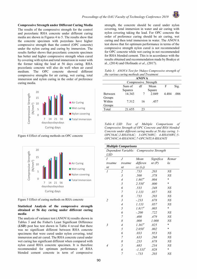
Proceedings of the OAU Faculty of Technology Conference 2019
90
Compressive Strength under Different Curing Media The results of the compressive strength for the control and pozzolanic RHA concrete under different curing media are shown in Figures 4 to 5. The results show that the concrete specimen with pozzolans have higher compressive strength than the control (OPC concrete) under the nylon curing and curing by immersion. The results further shows that pozzolanic concrete specimen has better and higher compressive strength when cured by covering with nylon and total immersion in water with the former taking the lead at 56 days curing. RHA pozzolanic concrete will also do well when air cured medium. The OPC concrete showed different compressive strengths for air curing, wet curing, total immersion and nylon curing in the order of preference curing media.
Figure 4 Effect of curing methods on OPC concrete
Figure 5 Effect of curing methods on RHA concrete
Statistical Analysis of the compressive strength obtained at 56 day curing under different curing media The analysis of variance test (ANOVA) results shown in Tables 3 and the Fisher's Least Significant Difference (LSD) post hoc test shown in Table 4 reveal that there was no significant different between RHA concrete specimens that were cured under nylon covering, total immersion and air cured. The RHA concrete cured under wet curing has significant different when compared with nylon cured RHA concrete specimen. It is therefore recommended for optimum performance of RHA blended cement concrete in term of compressive
strength, the concrete should be cured under nylon covering, total immersion in water and air curing with nylon covering taking the lead. For OPC concrete the order of preference curing should be air curing, wet curing and then total immersion in water. The ANOVA test shows that for optimum performance in terms of the compressive strength nylon cured is not recommended for OPC concrete while wet curing in not recommended for RHA blended cement. This is in accordance with the results obtained and recommendation made by Boakye et al., (2014) and Olofinade et al., (2017). Table 3: ANOVA Test for 56days Compressive strength of the various curing methods and Treatment
ANOVA Compressive_Strength
Sum of Squares
df Mean Square
F Sig.
Between Groups
14.343 7 2.049 4.484 .006
Within Groups
7.312 16 .457
Total 21.655 23
Table 4: LSD Test of Multiple Comparisons of Compressive Strength of OPC Concrete and RHA blended Concrete under different curing media at 56 day curing. 1-OPC56AC;2-RHA56AC; 3-OPC56WC; 4-RHA56WC;5-OPC56NC;6-RHA56NC;7-OPC56TI;8-RHA56TI
Multiple Comparisons Dependent Variable: Compressive Strength LSD I treatment
J treatment
Mean difference (i-j)
Significant (P)
Remarks
1 2 .733 .203 NS 3 .500 .378 NS 4 1.867* .004 * 5 2.550* .000 * 6 .533 .348 NS 7 1.133 .057 NS 8 .733 .203 NS 2 3 -.233 .678 NS 4 1.133 .057 NS 5 1.817* .005 * 6 -.200 .722 NS 7 .400 .479 NS 8 .000 1.000 NS 3 4 1.367* .025 * 5 2.050* .002 * 6 .033 .953 NS 7 .633 .268 NS 8 .233 .678 NS 4 5 .683 .234 NS 6 -1.333* .028 * 7 -.733 .203 NS
0
5
10
15
20
7days
14days
21days
56daysC
om
pre
sssi
ve S
tren
gth
(N
/mm
2)
Curing days
Air Curing
Wet curing
Nylon covering
Total Immersion
0
5
10
15
20
7days
14days
21days
56days
Co
mp
ress
ive
Stre
ngt
h
(N/m
m2 )
Curing days
Air Curing
Wet curing
Nylon covering
Total Immersion
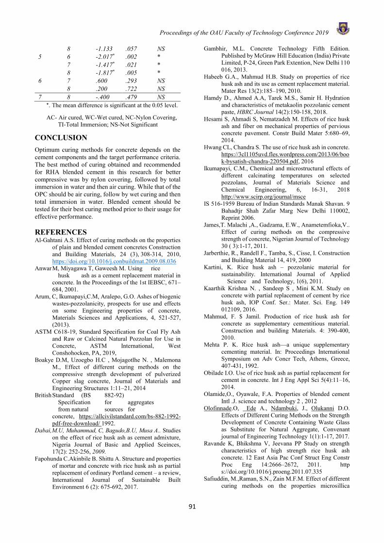
Proceedings of the OAU Faculty of Technology Conference 2019
91
8 -1.133 .057 NS 5 6 -2.017* .002 * 7 -1.417* .021 * 8 -1.817* .005 * 6 7 .600 .293 NS 8 .200 .722 NS 7 8 -.400 .479 NS
*. The mean difference is significant at the 0.05 level.
AC- Air cured, WC-Wet cured, NC-Nylon Covering, TI-Total Immersion; NS-Not Significant
CONCLUSION Optimum curing methods for concrete depends on the cement components and the target performance criteria. The best method of curing obtained and recommended for RHA blended cement in this research for better compressive was by nylon covering, followed by total immersion in water and then air curing. While that of the OPC should be air curing, follow by wet curing and then total immersion in water. Blended cement should be tested for their best curing method prior to their usage for effective performance. REFERENCES Al-Gahtani A.S. Effect of curing methods on the properties
of plain and blended cement concretes Construction and Building Materials, 24 (3), 308-314, 2010, https://doi.org/10.1016/j.conbuildmat.2009.08.036
Anwar M, Miyagawa T, Gaweesh M. Using rice husk ash as a cement replacement material in concrete. In the Proceedings of the 1st IEBSC, 671–684, 2001.
Arum, C, Ikumapayi,C.M, Aralepo, G.O. Ashes of biogenic wastes-pozzolanicity, prospects for use and effects on some Engineering properties of concrete, Materials Sciences and Applications, 4, 521-527, (2013).
ASTM C618-19, Standard Specification for Coal Fly Ash and Raw or Calcined Natural Pozzolan for Use in Concrete, ASTM International, West Conshohocken, PA, 2019,
Boakye D.M, Uzoegbo H.C , Mojagotlhe N. , Malemona M., Effect of different curing methods on the compressive strength development of pulverized Copper slag concrete, Journal of Materials and Engineering Structures 1:11–21, 2014
British Standard (BS 882-92) Specification for aggregates from natural sources for concrete, https://allcivilstandard.com/bs-882-1992-pdf-free-download/ 1992.
Dabai,M.U, Muhammad, C, Bagudo,B.U, Musa A.. Studies on the effect of rice husk ash as cement admixture, Nigeria Journal of Basic and Applied Sceinces, 17(2): 252-256, 2009.
Fapohunda C.Akinbile B. Shittu A. Structure and properties of mortar and concrete with rice husk ash as partial replacement of ordinary Portland cement – a review, International Journal of Sustainable Built Environment 6 (2): 675-692, 2017.
Gambhir, M.L. Concrete Technology Fifth Edition. Published by McGraw Hill Education (India) Private Limited, P-24, Green Park Extention, New Delhi 110 016, 2013.
Habeeb G.A., Mahmud H.B. Study on properties of rice husk ash and its use as cement replacement material. Mater Res 13(2):185–190, 2010.
Hamdy D., Ahmed A.A, Tarek M.S., Samir H. Hydration and characteristics of metakaolin pozzolanic cement paste, HBRC Journal 14(2):150-158, 2018.
Hesami S, Ahmadi S, Nematzadeh M. Effects of rice husk ash and fiber on mechanical properties of pervious concrete pavement. Constr Build Mater 5:680–69, 2014.
Hwang CL, Chandra S. The use of rice husk ash in concrete. https://3cl1105uvd.fles.wordpress.com/2013/06/book-bysatish-chandra-220504.pdf, 2016
Ikumapayi, C.M., Chemical and microstructural effects of different calcinating temperatures on selected pozzolans, Journal of Materials Science and Chemical Engineering, 6, 16-31, 2018 http://www.scirp.org/journal/msce
IS 516-1959 Bureau of Indian Standards Manak Shavan. 9 Bahadtjr Shah Zafar Marg New Delhi 110002, Reprint 2006.
James,T. Malachi ,A., Gadzama, E.W., Anametemfioka,V.. Effect of curing methods on the compressive strength of concrete, Nigerian Journal of Technology 30 ( 3):1-17, 2011.
Jarberthie, R., Randell F., Tamba, S., Cisse, I. Construction and Building Material 14, 419, 2000
Kartini, K. Rice husk ash – pozzolanic material for sustainability. International Journal of Applied Science and Technology, 1(6), 2011.
Kaarthik Krishna N. , Sandeep S , Mini K.M. Study on concrete with partial replacement of cement by rice husk ash, IOP Conf. Ser.: Mater. Sci. Eng. 149 012109, 2016.
Mahmud, F. $ Jamil. Production of rice husk ash for concrete as supplementary cementitious material. Construction and building Materials. 4: 390-400, 2010.
Mehta P. K. Rice husk ash—a unique supplementary cementing material. In: Proceedings International Symposium on Adv Concr Tech, Athens, Greece, 407-431, 1992.
Obilade I.O. Use of rice husk ash as partial replacement for cement in concrete. Int J Eng Appl Sci 5(4):11–16, 2014.
Olamide,O., Oyawale, F.A. Properties of blended cement Intl .J. science and technology 2 , 2012
Olofinnade.O, Ede A., Ndambuki, J., Olukanni D.O. Effects of Different Curing Methods on the Strength Development of Concrete Containing Waste Glass as Substitute for Natural Aggregate, Convenant journal of Engineering Technology 1(1):1-17, 2017.
Ravande K, Bhikshma V, Jeevana PP Study on strength characteristics of high strength rice husk ash concrete. 12 East Asia Pac Conf Struct Eng Constr Proc Eng 14:2666–2672, 2011. http s://doi.org/10.1016/j.proeng.2011.07.335
Safiuddin, M.,Raman, S.N., Zain M.F.M. Effect of different curing methods on the properties microsillica

Proceedings of the OAU Faculty of Technology Conference 2019
92
concrete, Australian Journal of basic and applied sciences, 1 (2): 87-95, 2007.
Sata V, Jaturapitakkul C, Kiattikomol K. Influence of pozzolan from various by-product materials on mechanical properties of high-strength concrete. Constr Build Mater 21(7):1589–1598, 2007.
Shivaram, M.S., (2014). Measures to Contain Pollution Caused Due to Cement Productions:-A review.
International Journal of Emerging Technology and Advanced Engineering, 4(11): 69-72
Dabai,M.U, Muhammad, C, Bagudo,B.U, Musa A. Studies on the Effect of Rice Husk Ash as Cement Admixture, Nigeria Journal of Basic and Applied Sceinces, 17(2): 252-256, 2009.
Proceedings of the OAU Faculty of Technology Conference 2019
93
ESTIMATION OF SHEAR STRENGTH PARAMETERS OF BANDED GNEISS DERIVED SOIL USING SELECTED INDEX PROPERTIES
G. O. Adunoye1,*, O. A. Agbede2 and M. O. Olorunfemi3 1Department of Civil Engineering, Obafemi Awolowo University, Ile-Ife, Nigeria
2Department of Civil Engineering, University of Ibadan, Ibadan, Nigeria 3Department of Geology, Obafemi Awolowo University, Ile-Ife, Nigeria
*Email of Corresponding Author: [email protected]
ABSTRACT This study developed models for predicting the shear strength parameters (cohesion, c and angle of internal friction, ϕ) of Banded Gneiss derived soils. This was with a view to establishing relationships between shear strength parameters and selected index properties; and reducing cost and time in the determination of geotechnical data needed for foundation analysis and design. A total of 25 soil samples were collected from selected locations within the Banded Gneiss environment of Obafemi Awolowo University (OAU) campus, Ile-Ife. The soils were subjected to preliminary, index property and engineering property tests, following standard procedures. The data obtained from the laboratory tests were subjected to stepwise regression, after which some index properties were identified and correlated with shear strength parameters, using Xuru’s regression tool. Twenty of the samples were used for model development while the remaining five samples were used for validation. The results showed that the cohesion of the soil samples ranged from 27 kN/m2 to 52 kN/m2, with a mean value of 35.4 kN/m2; while the angle of internal friction ranged from 6o to 19o, with a mean value of 13.32o. The results of stepwise regression, modelling and validation showed that uniformity coefficient, specific gravity and plasticity index predicted cohesion better; and effective size, uniformity coefficient and plasticity index predicted angle of internal friction better. The study concluded that the selected properties could be used to predict the shear strength parameters of soils in the study area. Keywords: Angle of internal friction, banded gneiss, cohesion, parameters, shear strength INTRODUCTION Shear strength of soil is its ability to resist sliding along internal surfaces within a mass, that is, the shear resistance offered by the soil along probable surfaces of slippape (Roy and Dass, 2014). Therefore, the stability of structures built on soil depends on the engineering properties, which includes shear strength. The shear strength of soil is generally expressed by the Mohr-Coulomb theory. According to this theory, the shear strength of soil varies linearly with the applied stress through two shear strength components known as the cohesion intercept (the intercept of Mohr-Coulomb failure envelope) (c) and angle of internal friction (the slope of Mohr-Coulomb failure envelope, expressed in degree) (ϕ). These two parameters are referred to as shear strength parameters of soil. The angle of internal friction gives an indication of the interlocking between the soil particles, while cohesion is due to the intermolecular bond between the adsorbed water surrounding each grain, especially in fine-grained soils (Arora, 1988; Murthy, 2008; and Mollahassani et al., 2011; Roy and Dass, 2014). Estimation of the shear strength parameters of soil is required for the design of foundations, retaining walls, and road pavements in civil engineering applications and for determining the resistance to traction and tillage tools in agricultural applications (Freudlund and Vanapali,
2002). These parameters are also essential in assessing the stability of slope of soil, and can be used to understand the ability of a soil to withstand stresses and strains associated with naturally occurring instances of increased pore pressure, cracking, swelling, development of slicken slides, leaching, weathering, undercutting, and cyclic loading, as well as anthropogenc changes to the landscape (Duncan and Wright, 2005). Failure of engineering structures (such as retaining wall, road pavement) and slope failure may be attributed, in part, to design error resulting from incorrect estimation of the shear strength parameters of the soil. Existing methods for the determination of shear strength parameters are based on tests that involve time, money and elaborate laboratory procedures. In other words, experimental determination of these parameters is cumbersome and costly (El-Maksoud, 2006; Murthy, 2008; Mousavi et al., 2011; Mollahassani et al., 2011; Adunoye, 2017). Since the index property tests of soils are relatively simple to perform, attempts have been made in the past to develop models for the determination of shear strength parameters of soil from the index properties (Cola and Cortellazo, 2005; Hajarwish and Shakor, 2006; Bareither et al., 2008; Masada, 2009; Mofiz and Rahman, 2010; Sorensen and Okkels, 2013; Adunoye, 2014a and b) . However, the previous attempts are region-specific and thus necessitate the need for localized investigation. There is also the need to develop

Proceedings of the OAU Faculty of Technology Conference 2019
94
models (which will be applicable across regions, on the basis of lithology units) that can be easily employed for determining cohesion and angle of internal friction. Hence this study.
Description and geology of the study area The study area is the Obafemi Awolowo (OAU) campus, Ile-Ife, Southwestern Nigeria. The OAU campus is located within the Ife-Ilesha Schist Belt. The campus falls within the Basement Complex area of Nigeria (Durotoye, 1983). According to Boesse (1989), the rock types are primarily made up of Gneisses and Mica Schists into which some minor granitic and basic rocks have intruded. The main lithological units are: Banded Gneiss, Granite Gneiss and Mica Schist. Figure 1 shows the geological map of OAU.
MATERIALS AND METHODS Materials and equipment The main materials used are lateritic soil samples collected from Banded Gneiss geologic unit in the study area. The list of equipment used is contained in Table 1. They are all available at the Geotechnical Engineering Laboratory of Department of Civil Engineering,
Obafemi Awolowo University, Ile-Ife (Adunoye, 2017; Adunoye et al., 2018).
Figure 1: Geological Map of the Obafemi Awolowo University, Ile-Ife (After Boesse, 1989) METHOD Twenty-five sampling locations were identified within Banded Gneiss geologic unit in the study area.
Table 1: List of equipment
Equipment Purpose
Set of Sieves (4.5mm to 0.06mm) Particle size analysis (coarse grain)
Sieve Shaker Shaking of soil sieves Hydrometer Bulb Particle size analysis (fine grain) Specific Gravity Bottle Specific gravity determination
Atterberg Apparatus Plastic and liquid limits determination Electric Oven (Temp 105oC to 110oC) Drying of moist soil sample Weighing balance Weighing of soil Measuring Cans Measurement Compaction Moulds and Rammers Compaction test
Triaxial Machine Determination of shear strength parameters
The soil samples were collected at approximately one sample per 200 m2. Test pits were dug by hand and excavated with the aid of digger and shovel. The depth of sample collection was 0.5 m – 1 m (Arora, 1988; Roy and Das, 2014). 20 - 25 kg of each sample was collected into a nylon, sealed and immediately taken to the Geotechnical Laboratory of the Department of Civil Engineering, OAU, Ile-Ife, for analyses. In the Laboratory, representative samples were taken and used for the determination of natural moisture content. After determining the natural moisture content, the samples were prepared for subsequent laboratory analyses by air-drying and grinding to pass a 2 mm sieve.
Further geotechnical analyses/tests carried out on soil samples included: particle size analysis, specific gravity test, and Atterberg limits test. All tests and analyses were conducted following standard procedures as contained in BS 1377 (1990). Effectives sizes (D10, D30 and D60), uniformity coefficient (Cu) and Coefficient of curvature (Cc) were also determined from the particle size distribution curves and Equations 1 and 2.
Cc = D302/(D60 x D10) (1)
Cu = D60/D10 (2) Where D10 = Grain size for which 10% of the
sample is finer
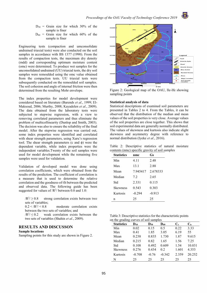
Proceedings of the OAU Faculty of Technology Conference 2019
95
D30 = Grain size for which 30% of the sample is finer
D60 = Grain size for which 60% of the sample is finer
Engineering tests (compaction and umconsolidate undrained triaxial tests) were also conducted on the soil samples in accordance with BS 1377 (1990). From the results of compaction tests, the maximum dry density (mdd) and corresponding optimum moisture content (omc) were determined. To produce wet samples for the unconsolidated undrained (UU) triaxial tests, the dry soil samples were remoulded using the omc value obtained from the compaction tests. UU triaxial tests were subsequently conducted on the remoulded soil samples. The soil cohesion and angle of internal friction were then determined from the resulting Mohr envelope. The index properties for model development were considered based on literature (Barends et al., 1999; El-Maksoud, 2006; Murthy, 2008; Kayadelen et al., 2009). The data obtained from the laboratory tests were subjected to stepwise regression, with a view to removing correlated parameters and thus eliminate the problem of multicollinearity (Dunlop and Smith, 2003). The decision was also to ensure the reliability of the final model. After the stepwise regression was carried out, some index properties were identified and correlated with shear strength parameters, using Xuru’s regression tool. The shear strength parameters (c and ϕ) were the dependent variable, while index properties were the independent variables.Twenty of the soil samples were used for model development while the remaining five samples were used for validation. Validation of developed model was done using correlation coefficients, which were obtained from the results of the prediction. The coefficient of correlation is a measure that is used to determine the relative correlation and the goodness-of-fit between the predicted and observed data. The following guide has been suggested for values of /R2/ between 0.0 and 1.0:
/R2/ ≥ 0.8 strong correlation exists between two sets of variables; 0.2 < /R2/ < 0.8 moderate correlation exists between the two sets of variables; and /R2/ ≤ 0.2 weak correlation exists between the two sets of variables (Shahin et al., 2009).
RESULTS AND DISCUSSON Sample locations Sampling points for this study are shown in Figure 2.
Figure 2: Geological map of the OAU, Ile-Ife showing sampling points Statistical analysis of data Statistical descriptions of examined soil parameters are presented in Tables 2 to 4. From the Tables, it can be observed that the distribution of the median and mean values of the soil properties is very close. Average values of the soil properties are close together. This shows that soil experimental data are generally normally distributed. The values of skewness and kurtosis also indicate slight skewness and asymmetry degree with reference to normal distribution (Iyeke et al., 2016). Table 2: Descriptive statistics of natural moisture contents (nmc) specific gravity of soil samples
Statistics nmc Gs Min 4.11 2.48 Max 13.1 2.88 Mean 7.945417 2.678333 Median 7.2 2.65 Std 2.331 0.115 Skewness 0.543 0.303 Kurtosis -0.294 -0.913 n 25 25
Table 3: Descriptive statistics for the characteristic points on the grading curves of soil samples
Statistics D10 D30 D60 Cc Cu Min 0.02 0.15 0.5 0.22 3.33 Max 0.41 1.85 3.05 6.19 55 Mean 0.238 0.835 1.730 1.87 9.615 Median 0.215 0.82 1.65 1.56 7.25 Std 0.108 0.492 0.609 1.54 10.031 Skewness 0.276 0.434 0.2 1.601 4.353 Kurtosis -0.708 -0.76 -0.342 2.359 20.252 N 25 25 25 25 25
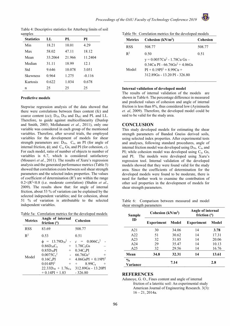
Proceedings of the OAU Faculty of Technology Conference 2019
96
Table 4: Descriptive statistics for Atterberg limits of soil samples
Statistics LL PL PI Min 18.21 10.01 4.29 Max 58.02 47.11 18.12 Mean 33.2064 21.966 11.2404 Median 31.11 18.99 12.1 Std 9.646 10.078 3.051 Skewness 0.964 1.275 -0.116 Kurtosis 0.622 1.034 0.678 n 25 25 25
Predictive models Stepwise regression analysis of the data showed that there were correlations between fines content (fc) and coarce content (cc); D10, D30 and D60; and PL and LL. Therefore, to guide against multicollinearity (Dunlop and Smith, 2003; Mollahasani et al., 2011), only one variable was considered in each group of the mentioned variables. Therefore, after several trials, the employed variables for the development of models for shear strength parameters are: D30, Cu, an PI (for angle of internal friction, ϕ); and Cu, Gs, and PI (for cohesion, c). For each model, ratio of number of objects to number of variables is 6.7, which is considered satisfactory (Mousavi et al., 2011). The results of Xuru’s regression analysis and the generated performance metrics (Table 5) showed that correlation exists between soil shear strength parameters and the selected index properties. The values of coefficient of determination (R2) are within the range 0.2<(R2<0.8 (i.e. moderate correlation) (Shahin et al., 2009). The results show that: for angle of internal friction, about 53 % of variation can be explained by the selected independent variables; and for cohesion, about 51 % of variation is attributable to the selected independent variables. Table 5a: Correlation metrics for the developed models
Metrics Angle of internal friction (o) Cohesion
RSS 83.69 508.77
R2 0.53 0.51
Model
ϕ = 13.79D302 -
0.86D30Cu + 0.85D30PI + 0.0075Cu
2 - 0.16CuPI + 0.014PI2 + 22.33D30 + 1.76Cu + 0.14PI + 1.83
c = 0.006Cu2 -
1.78CuGs – 0.34CuPI - 66.76Gs2 + 4.06GsPI + 0.19PI2 + 8.99Cu + 312.89Gs - 13.20PI - 326.80
Table 5b: Correlation metrics for the developed models
Metrics Cohesion (kN/m2) Cohesion
RSS 508.77 508.77
R2 0.50 0.51
Model
y = 0.0057Cu2 - 1.78Cu Gs – 0.34Cu PI - 66.76Gs2 + 4.06Gs PI + 0.19PI2 + 8.99Cu + 312.89Gs - 13.20 PI - 326.80
Internal validation of developed model The results of internal validation of the models are shown in Table 6. The percentage difference in measured and predicted values of cohesion and angle of internal friction is less than 8%, thus considered low (Ayininuola et. al, 2009). Therefore, the developed model could be said to be valid for the study area. CONCLUSION This study developed models for estimating the shear strength parameters of Banded Gneiss derived soils, using selected index properties. After experimental tests and analyses, following standard procedures, angle of internal friction model was developed using D30, Cu, and PI; while cohesion model was developed using Cu, Gs, and PI. The models were developed using Xuru’s regression tool. Internal validation of the developed models showed that they were found valid for the study area. Since the coefficients of determination for the developed models were found to be moderate, there is need for further work to examine the contribution of other soil properties in the development of models for shear strength parameters.
Table 6: Comparison between measured and model shear strength parameters
Sample ID
Cohesion (kN/m2) Angle of internal friction (o)
Experiment Model Experiment Model
A21 30 34.06 14 3.78 A22 51 30.62 14 17.31 A23 32 31.85 14 20.06 A24 29 35.47 14 10.13 A25 32 29.56 14 16.76
Mean 34.8 32.31 14 13.61 % Variance 7.14 2.8
REFERENCES Adunoye, G. O., Fines content and angle of internal
friction of a lateritic soil: An experimental study American Journal of Engineering Research. 3(3): 16 – 21, 2014a.
Proceedings of the OAU Faculty of Technology Conference 2019
97
Adunoye, G. O., Study of relationship between fines content and cohesion of soil. British Journal of Applied Science and Technology. 4(4): 682 – 692, 2014b.
Adunoye, G. O., Development of predictive models for determining the shear strength of lateritic soils in a Basement Complex environment. Unpublished Ph.D Thesis, department of Civil Engineering, Obafemi Awolowo University, Ile-Ife, 2017.
Adunoye, G. O., Agbede, O. A., and Olorunfemi, M. O., Development of shear strength model for Banded Gneiss derived soils. IOSR Journal of Applied Geology and Geophysics, 6(6): 14 – 24, 2018.
Arora, K. R., Introductory Soil Engineering. Nem Chand Jane (Prop), Standard Publishers Distributors, Nai Sarak, Delhi, 1988.
Ayininuola, G. M., Agbede, O. A. and Franklin, S. O.. Influence of calcium sulphate on subsoil cohesion and angle of friction, Journal of Applied Sciences Research, 5(3): 297 – 304, 2009.
Bareither, C. A., Geological and physical factors affecting the friction angle of compacted sands, Journal of Geotechnical and Geoenvironmental Engineering, 134 (10): 1476-1489, 2008.
Barends, F. B. J., Lindenberg, J. L., De Quelerij, L., Verruijt, A. and Luger, H. J, Geotechnical Engineering for Transportation Infrastructure: Theory and Practice, Planning and Design, Construction and Maintenance; Balkema Publishers, Netherlands, 1999.
Boesse, J. M., A Geological map of the Obafemi Awolowo University Campus (Unpublished), Department of Geology, Obafemi Awolowo University, Ile-Ife, 1989.
BS 1377, Methods of test for soils for civil engineering properties. British Standard Institution, London, 1990.
Cola, S. and Cortellazzo, G., The shear strength behavior of two peaty soils. Geotechnical and Geological Engineering, 23:679-695, 2005.
Duncan, J. M. and Wright, S. G., Soil strength and slope stability, John Wiley & Sons, New York, 2005.
Dunlop, P. and Smith, S., Estimating key characteristics of the concrete delivery and placement process using linear regression analysis. Civil Eng. Environ. Syst., 20: 273-290, 2003.
Durotoye, A. B., Quarternary Sediments in Nigeria. Edited by Kogbe C. A, 1983.
El-Maksoud, M. A. F., Laboratory determining of soil strength parameters in calcareous soils and their effect on chiseling draft prediction. In: Proceedings of Energy Efficiency and Agricultural Engineering International Conference, Rousse, Bulgaria, 2006.
Fredlund, D. G. and Vanapalli, S. K. Shear strength of unsaturated soils. Agronomy Society of America, pp. 329-361, 2002.
Hajdarwish, A. and Shakoor, A. Predicting the shear strength parameters of mudrocks.The Geological Society of London. IAEG Paper number 607, 2006.
Iyeke, S. D. Eze, E. O., Ehiorobo, J. O., and Osuji, S. O., Estimation of shear strength parameters of lateritic soils using artificial neural network, Nigerian Journal of Technology, 35(2): 260-269, 2006.
Kayadelen, C., G¨unaydın, O., Fener, M., Demir, A. and ¨Ozvan, A., A modeling of the angle of shearing resistance of soils using soft computing systems, Expert. Syst. Appl., 36: 11,814–11,826, 2009.
Masada, T., Shear strength of clay and silt embankments. Ohio Research Institute for Transportation and the Environment. Ohio University, Ohio, 2009.
Mofiz, S. A. and Rahman M. M., Shear strength behavior of barind soil on triaxial extension stress path tests.: 11th IAEG Congress, Auckland, New Zealand, pp 2249-2256, 2010.
Mollahasani, A., Alavi, A. H, Gandomi, A. H. and Rashed, A., Nonlinear neural-based modeling of soil cohesion intercept. KSCE Journal of Civil. Engineering., 15(5): 831–840, 2011.
Mousavi, S.M., Alavi, A.H., Gandomi, A.H. and Mollahasani, A., Nonlinear genetic-based simulation of soil shear strength parameters, J. Earth Syst. Sci., 120(6): 1001-1022, 2011.
Murthy, S., Geotechnical Engineering: Principles and Practices of Soil Mechanics. 2nd edition, Taylor & Francis, CRC Press, UK, 2008.
Roy, S. and Dass, G., Statistical models for the prediction of shear strength parameters of Sirsa, India. International Journal of Civil and Structural Engineering, 4(4): 483 – 498, 2014.
Shahin, M. A., Jaksa, M. B. and Maier, H. R., Recent advances and future challenges for artificial neural systems in geotechnical engineering applications. Adv. Artif. Neur. Syst., Article ID 308239, 2009.
Sorensen, K. K. and Okkels, N., Correlation between drained shear strength and plasticity index of undisturbed over consolidated clays. Proceedings of the 18th International Conference on Soil Mechanics and Geotechnical Engineering, Paris, 2013, pp. 1-6, 2013.
Proceedings of the OAU Faculty of Technology Conference 2019
98
LOAD-DEFORMATION OF KENAF (HIBISCUS CANNABINUS) STEM AT DIFFERENT MATURITY STAGES
O. B. Falana*1; A. O. Adeboboye1; I. O. Adanike1, T. M. Olagunju1 1Department of Agricultural and Environmental Engineering,
Obafemi Awolowo University, Ile-Ife, Osun State, Nigeria
*Email of Corresponding Author: [email protected]
ABSTRACT
This study determined the stress deformation characteristics of kenaf stems harvested at three different stages of maturity (12, 16 and 20 weeks) with the view to providing useful information for the usage as a structural material and the design of appropriate handling machines for kenaf and other similar plants. Two kenaf varieties (Ifeken 100 and Tianung 1) were harvested from the Teaching and Research Farms, Obafemi Awolowo University, Ile-Ife, Nigeria. Some mechanical properties of the stems were determined using appropriate apparatus and standard procedures. The maximum bending strength, shearing load, shearing energy, and Young’s modulus of Tianung 1 were 52.40 MPa, 304.18 N, 5.89 J.mm-2, and 521.28 MPa, while the corresponding values for Ifeken 100 were 19.60 MPa, 205.36 N, 2.96 J.mm-2, and 350.06 MPa, respectively. The lowest moisture content of Tianung 1 was 16.60% (wb) while Ifeken 100 was 13.99% (wb) at 20 weeks of maturity. The moisture content of the two kenaf varieties reduced significantly while the bending strength, shearing load, shearing energy, and Young’s modulus increased with maturity. Keywords: Kenaf, Bending Strength, Shearing Load, Shearing Energy, Ifeken 100, Tianung 1 INTRODUCTION Kenaf is a warm-season annual fibre crop closely related to cotton and jute. It has a cellulosic source with both economic and ecological advantages. It could grow under a wide range of weather condition to a height of more than 3 m and a base diameter of 3 – 5 cm (Webber et al., 2002). Kenaf has a single, straight, unbranched stem consisting of two parts, namely outer fibrous bark and inner woody core. Kenaf comprises 35 - 40% bast fibre and 60 – 65% core fibres by weight of the stalk. Kenaf contains approximately 65.7% cellulose, 21.6% lignin and pectin, and other composition (Mohanty et al., 2004). Kenaf has excellent mechanical properties and can proliferate as it takes only 12 to 20 weeks to harvest depending on the best condition for fibre and seeds. Studies on the usage of kenaf have long been the subject of discussion and critique of scientific discovery and have attracted the attention of researchers globally because of its economic significance. Some researchers focused on the exploitation of the plant because of its homogenous blend with resins used as plastic composites, as a drilling fluid loss preventative for oil drilling muds, others, for a seeded hydro-mulch for erosion control, for a seeded grass mats for instant lawns and mouldable mats for manufactured parts and containers (Webber et al., 2002). Kenaf has also been used as a cordage crop to produce twine, rope, and sackcloth. Nowadays, there are various new applications for kenaf, including animal feeds, building materials, absorbents, and paper products. For paper production, Nishino et al. (2003) stated that chemically extracted bast pulp is well
suited for specialty papers, such as high-quality stationery or filter paper. In term of strength, the bast pulp, compared to softwood pulp, has similar tensile strength, but greater tear strength, thus it could serve as a replacement for softwood pulp. Despite the increasing global demand for kenaf, there is a dearth of information on the physical and mechanical properties of kenaf which could help researchers design and develop appropriate post-harvest machines as well as optimization as a structural material. However, this study seeks to provide the necessary information that could enhance kenaf usage as a structural material, development of machines and processes for handling, and harvesting kenaf stems at different maturity stages. Hence, the objective of the study was to investigate the effects of harvesting time on the moisture content level and some mechanical properties including the bending strength, shearing load, shearing energy, and Young’s modulus of kenaf stem.
MATERIAL AND METHODS Samples preparation In this research, the moisture content and mechanical properties of two kenaf varieties (Ifeken 100 and Tianung 1) were studied at three stages of plant maturity (12, 16, and, 20 weeks). The kenaf seeds were sourced from the Institute of Agricultural Research and Training, Ibadan, Nigeria, and were planted at the Teaching and Research Farms, Obafemi Awolowo University, Ile-Ife, Nigeria. At each stage of maturity, the test specimens were harvested at the height of 10 cm above ground level (Kayembe, 2015) and were transferred to the Department of Agricultural and Environmental Engineering laboratory.
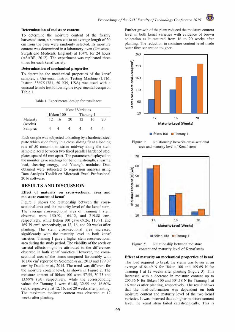
Proceedings of the OAU Faculty of Technology Conference 2019
99
Determination of moisture content To determine the moisture content of the freshly harvested stem, six stems cut to an average length of 20 cm from the base were randomly selected. Its moisture content was determined in a laboratory oven (Uniscope, Surgifriend Medicals, England) at 104⁰C for 24 hours (ASABE, 2012). The experiment was replicated three times for each kenaf variety. Determination of mechanical properties To determine the mechanical properties of the kenaf samples, a Universal Instron Testing Machine (UTM, Instron 3369K1781, 50 KN, USA) was used with a uniaxial tensile test following the experimental design on Table 1.
Table 1: Experimental design for tensile test
Kenaf Varieties Ifeken 100 Tianung 1 Maturity (weeks)
12 16 20 12 16 20
Samples 4 4 4 4 4 4 Each sample was subjected to loading by a hardened steel plate which slide freely in a close sliding fit at a loading rate of 50 mm/min to strike midway along the stem sample placed between two fixed parallel hardened steel plates spaced 65 mm apart. The parameters displayed on the monitor gave readings for bending strength, shearing load, shearing energy, and Young’s modulus. Data obtained were subjected to regression analysis using Data Analysis Toolkit on Microsoft Excel Professional 2016 software.
RESULTS AND DISCUSSION Effect of maturity on cross-sectional area and moisture content of kenaf Figure 1 shows the relationship between the cross-sectional area and the maturity level of the kenaf stem. The average cross-sectional area of Tianung 1 stem observed were 150.92, 164.12, and 219.88 cm2, respectively, while Ifeken 100 gave 69.26, 110.91, and 169.39 cm2, respectively, at 12, 16, and 20 weeks after planting. The stem cross-sectional area increased significantly with the maturity level in both kenaf varieties. Tianung 1 gave a higher stem cross-sectional area during the study period. The viability of the seeds or varietal effects might be attributed to the differences observed in both kenaf varieties. However, the cross-sectional area of the stems compared favourably with 161.06 cm2 reported by Solomon et al., 2013 and 179.09 cm2 by Dauda et al., 2014. The trend was different for the moisture content level, as shown in Figure 2. The moisture content of Ifeken 100 were 57.55, 30.73 and 13.99% (wb) respectively, while the corresponding values for Tianung 1 were 61.48, 32.55 and 16.60% (wb), respectively, at 12, 16, and 20 weeks after planting. The maximum moisture content was observed at 12 weeks after planting.
Further growth of the plant reduced the moisture content level in both kenaf varieties with evidence of brown coloration as it matured from 16 to 20 weeks after planting. The reduction in moisture content level made outer fibre separation tougher.
Figure 1: Relationship between cross-sectional
area and maturity level of Kenaf stem
Figure 2: Relationship between moisture
content and maturity level of Kenaf stem
Effect of maturity on mechanical properties of kenaf The load required to break the stems was lower at an average of 64.49 N for Ifeken 100 and 109.69 N for Tianung 1 at 12 weeks after planting (Figure 3). This increased with a decrease in moisture content up to 205.36 N for Ifeken 100 and 304.18 N for Tianung 1 at 16 weeks after planting, respectively. The result shows that the load-deformation was dependent on both moisture content and maturity level of the two kenaf varieties. It was observed that at higher moisture content level, the kenaf stem failed catastrophically. This is
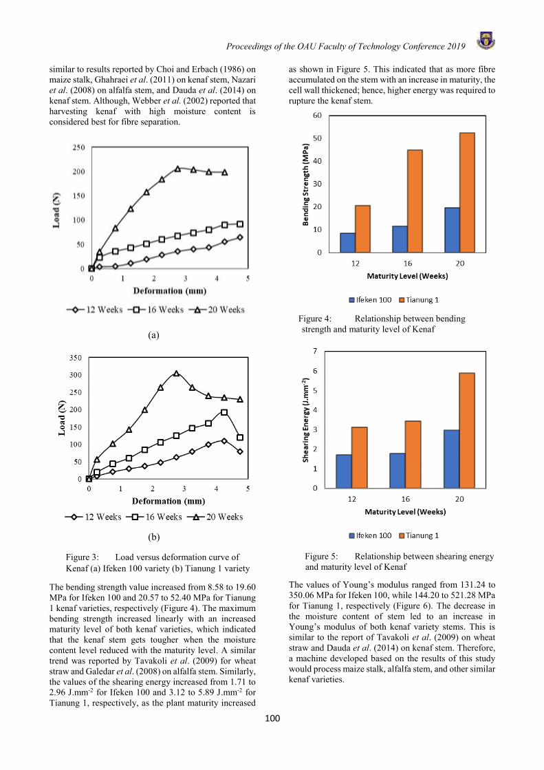
Proceedings of the OAU Faculty of Technology Conference 2019
100
similar to results reported by Choi and Erbach (1986) on maize stalk, Ghahraei et al. (2011) on kenaf stem, Nazari et al. (2008) on alfalfa stem, and Dauda et al. (2014) on kenaf stem. Although, Webber et al. (2002) reported that harvesting kenaf with high moisture content is considered best for fibre separation.
(a)
(b)
Figure 3: Load versus deformation curve of Kenaf (a) Ifeken 100 variety (b) Tianung 1 variety
The bending strength value increased from 8.58 to 19.60 MPa for Ifeken 100 and 20.57 to 52.40 MPa for Tianung 1 kenaf varieties, respectively (Figure 4). The maximum bending strength increased linearly with an increased maturity level of both kenaf varieties, which indicated that the kenaf stem gets tougher when the moisture content level reduced with the maturity level. A similar trend was reported by Tavakoli et al. (2009) for wheat straw and Galedar et al. (2008) on alfalfa stem. Similarly, the values of the shearing energy increased from 1.71 to 2.96 J.mm-2 for Ifeken 100 and 3.12 to 5.89 J.mm-2 for Tianung 1, respectively, as the plant maturity increased
as shown in Figure 5. This indicated that as more fibre accumulated on the stem with an increase in maturity, the cell wall thickened; hence, higher energy was required to rupture the kenaf stem.
Figure 4: Relationship between bending strength and maturity level of Kenaf
Figure 5: Relationship between shearing energy and maturity level of Kenaf
The values of Young’s modulus ranged from 131.24 to 350.06 MPa for Ifeken 100, while 144.20 to 521.28 MPa for Tianung 1, respectively (Figure 6). The decrease in the moisture content of stem led to an increase in Young’s modulus of both kenaf variety stems. This is similar to the report of Tavakoli et al. (2009) on wheat straw and Dauda et al. (2014) on kenaf stem. Therefore, a machine developed based on the results of this study would process maize stalk, alfalfa stem, and other similar kenaf varieties.
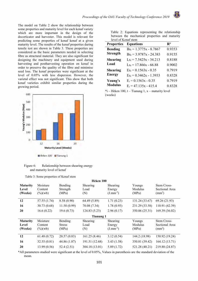
Proceedings of the OAU Faculty of Technology Conference 2019
101
The model on Table 2 show the relationship between some properties and maturity level for each kenaf variety which are more important in the design of the decorticator and harvester. This model is relevant for predicting some properties of kenaf kenaf at a given maturity level. The results of the kenaf properties during tensile test are shown in Table 3. These properties are considered as the basic parameters needed in selecting fibre as structural material. They are also significant for designing the machinery and equipment used during harvesting and postharvesting operation on kenaf in order to preserve the quality of the fibre and minimise seed loss. The kenaf properties were significant at the level of 0.05% with less dispersion. However, the varietal effect was not significant. This show that both kenaf varieties exhibit similar properties during the growing period.
Figure 6: Relationship between shearing energy and maturity level of kenaf
Table 2: Equations representing the relationship between the mechanical properties and maturity level of Kenaf stem
Properties Equations R² Bending Strength
Bsi = 1.3775x - 8.7867 0.9353 Bst = 3.9787x - 24.383 0.9155
Shearing Load
Lsi = 7.5425x - 34.213 0.8188 Lst = 17.866x - 66.88 0.9002
Shearing Energy
Esi = 0.1563x - 0.35 0.7919 Est = 0.3462x - 1.3933 0.8328
Young’s Modulus
Ei = 0.1563x - 0.35 0.7919 Et = 47.135x - 415.4 0.8328
*i – Ifeken 100, t – Tianung 1, x – maturity level (weeks)
Table 3: Some properties of Kenaf stem Ifeken 100
Maturity Level (Weeks)
Moisture Content (%)(wb)
Bending Strength (MPa)
Shearing Load (N)
Shearing Energy (J.mm-2)
Youngs Modulus (MPa)
Stem Cross-Sectional Area (mm2)
12 57.55 (1.74) 8.58 (0.90) 64.49 (5.89) 1.71 (0.23) 131.24 (33.67) 69.26 (21.93) 16 30.73 (0.68) 11.58 (0.99) 70.08 (7.34) 1.78 (0.93) 231.29 (33.58) 110.91 (42.39) 20 16.6 (0.22) 19.6 (0.73) 124.83 (5.23) 2.96 (0.17) 350.06 (25.31) 169.39 (36.02)
Tianung 1 Maturity Level (Weeks)
Moisture Content (%)(wb)
Bending Stress (MPa)
Shearing Load (N)
Shearing Energy (J.mm-2)
Youngs Modulus (MPa)
Stem Cross-Sectional Area (mm2)
12 61.48 (0.72) 20.57 (0.83) 161.25 (8.46) 3.12 (0.54) 144.2 (18.98) 150.92 (19.24) 16 32.55 (0.81) 44.86 (1.87) 191.51 (12.68) 3.43 (1.58) 350.81 (39.42) 164.12 (13.71) 20 13.99 (0.56) 52.4 (2.51) 304.18 (13.01) 5.89 (1.72) 521.28 (40.21) 219.88 (24.87)
*All parameters studied were significant at the level of 0.05%, Values in parenthesis are the standard deviation of the mean.
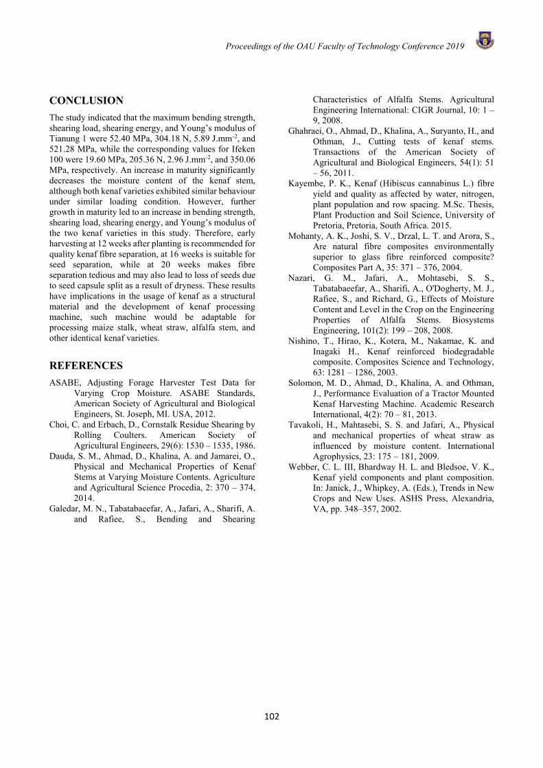
Proceedings of the OAU Faculty of Technology Conference 2019
102
CONCLUSION The study indicated that the maximum bending strength, shearing load, shearing energy, and Young’s modulus of Tianung 1 were 52.40 MPa, 304.18 N, 5.89 J.mm-2, and 521.28 MPa, while the corresponding values for Ifeken 100 were 19.60 MPa, 205.36 N, 2.96 J.mm-2, and 350.06 MPa, respectively. An increase in maturity significantly decreases the moisture content of the kenaf stem, although both kenaf varieties exhibited similar behaviour under similar loading condition. However, further growth in maturity led to an increase in bending strength, shearing load, shearing energy, and Young’s modulus of the two kenaf varieties in this study. Therefore, early harvesting at 12 weeks after planting is recommended for quality kenaf fibre separation, at 16 weeks is suitable for seed separation, while at 20 weeks makes fibre separation tedious and may also lead to loss of seeds due to seed capsule split as a result of dryness. These results have implications in the usage of kenaf as a structural material and the development of kenaf processing machine, such machine would be adaptable for processing maize stalk, wheat straw, alfalfa stem, and other identical kenaf varieties.
REFERENCES ASABE, Adjusting Forage Harvester Test Data for
Varying Crop Moisture. ASABE Standards, American Society of Agricultural and Biological Engineers, St. Joseph, MI. USA, 2012.
Choi, C. and Erbach, D., Cornstalk Residue Shearing by Rolling Coulters. American Society of Agricultural Engineers, 29(6): 1530 – 1535, 1986.
Dauda, S. M., Ahmad, D., Khalina, A. and Jamarei, O., Physical and Mechanical Properties of Kenaf Stems at Varying Moisture Contents. Agriculture and Agricultural Science Procedia, 2: 370 – 374, 2014.
Galedar, M. N., Tabatabaeefar, A., Jafari, A., Sharifi, A. and Rafiee, S., Bending and Shearing
Characteristics of Alfalfa Stems. Agricultural Engineering International: CIGR Journal, 10: 1 – 9, 2008.
Ghahraei, O., Ahmad, D., Khalina, A., Suryanto, H., and Othman, J., Cutting tests of kenaf stems. Transactions of the American Society of Agricultural and Biological Engineers, 54(1): 51 – 56, 2011.
Kayembe, P. K., Kenaf (Hibiscus cannabinus L.) fibre yield and quality as affected by water, nitrogen, plant population and row spacing. M.Sc. Thesis, Plant Production and Soil Science, University of Pretoria, Pretoria, South Africa. 2015.
Mohanty, A. K., Joshi, S. V., Drzal, L. T. and Arora, S., Are natural fibre composites environmentally superior to glass fibre reinforced composite? Composites Part A, 35: 371 – 376, 2004.
Nazari, G. M., Jafari, A., Mohtasebi, S. S., Tabatabaeefar, A., Sharifi, A., O'Dogherty, M. J., Rafiee, S., and Richard, G., Effects of Moisture Content and Level in the Crop on the Engineering Properties of Alfalfa Stems. Biosystems Engineering, 101(2): 199 – 208, 2008.
Nishino, T., Hirao, K., Kotera, M., Nakamae, K. and Inagaki H., Kenaf reinforced biodegradable composite. Composites Science and Technology, 63: 1281 – 1286, 2003.
Solomon, M. D., Ahmad, D., Khalina, A. and Othman, J., Performance Evaluation of a Tractor Mounted Kenaf Harvesting Machine. Academic Research International, 4(2): 70 – 81, 2013.
Tavakoli, H., Mahtasebi, S. S. and Jafari, A., Physical and mechanical properties of wheat straw as influenced by moisture content. International Agrophysics, 23: 175 – 181, 2009.
Webber, C. L. III, Bhardway H. L. and Bledsoe, V. K., Kenaf yield components and plant composition. In: Janick, J., Whipkey, A. (Eds.), Trends in New Crops and New Uses. ASHS Press, Alexandria, VA, pp. 348–357, 2002.
Proceedings of the OAU Faculty of Technology Conference 2019
103
MAPPING OF CARBON NANOTUBE DISPERSION IN BALL MILLED CNT-AL MIXED POWDERS
1U. Abdullah*, 2M. A. Maleque, 2M.Y. Ali and 2I. I. Yaacob 1Center for Energy Research and Training (Nigeria Atomic Energy Commission),
Ahmadu Bello University Zaria, P.M.B 1044 Samaru, Post code: 810107 Kaduna State, Nigeria
2Department of Manufacturing and Materials Engineering, Kulliyyah of Engineering, International Islamic University, P.O. Box 10, 50728 Kuala Lumpur, Malaysia
Emails: [email protected]
ABSTRACT Currently, carbon nanotubes (CNT) are attracting much interest as fibrous materials for reinforcing aluminium matrix composites due to unique properties such as high strength, elastic modulus, flexibility and high aspect ratios. However, the quality of the dispersion is a major concern factor that determines the homogeneity of the enhanced mechanical and tribological properties of the nano composite powders. This work studied and characterised carbon nanotube dispersion in ball milled CNT-Aluminium powders under high energy planetary ball milling operations. The ball milling was performed for two hours at constant milling speed of 250rpm under controlled atmosphere. The experimental results showed homogeneous dispersion of CNTs in aluminium powder. The characterisation was performed using FESEM and EDX analyser for mapping, elemental and line analyses. The compositions of 1.5, 2 and 2.5 wt% CNTs showed similar pattern from mapping analysis, elemental analysis and line analysis. Identification of only two peaks proved that control atmosphere during milling prevented the formation of inter metallic compounds such as aluminium carbide in the composite. Therefore this CNT-Al powder mix can be used for nano-composite development. Key words: Carbon nanotube, Aluminium powder, Dispersion, Characterisation, FESEM, EDX
INTRODUCTION Research in the field of carbon was revolutionised by the discovery of carbon nanotubes (CNTs) by Iijima, (1991). Although CNTs might have been synthesised in 1960 by Bacon, it took the genius of Iijima to realise that they are tubes made by rolling a graphene sheet onto itself. A multiwalled carbon nanotube (MWCNT) is made up of many single walled carbon nanotubes (SWCNT) arranged in a concentric manner. Experiments and simulations showed that CNTs have extraordinary mechanical properties over carbon fibres, e.g. stiffness of up to 1000 GPa, strength is in the order of 100 GPa Baksi et al. (2010), and thermal conductivity of up to 6000 W mK. Carbon nanotube reinforced metal matrix composites (CNT-MMC) are prepared using different type of processing techniques. Powder metallurgy (PM) is the most popular and widely used route by researchers to synthesise CNT-MMC materials. Aluminium (Al) matrix composite has wide prospects of application in aviation, spaceflight and automobile industries because of lower density as this is a mandatory for the weight reduction of the components thereby saving fuels and hence energy used. Carbon nanotube reinforced aluminium (CNT-Al) composites are mainly produced using powder metallurgy method. Ball milling is the easier and cheaper means of synthesization of composite materials powders in powder metallurgy route. Nano-composite materials are multiphase materials obtained through the artificial combination of different materials
either ceramic, polymeric or metallic matrices with carbon nanotubes to attain properties that the individual components by themselves cannot attain Poirer et al (2009) and Savage G. (1993). It is believed that graphitic type of carbon fibre enhances the thermal conductivity, mechanical and tribological property of the material significantly.
However, successful dispersion of CNTs in the metallic matrix is of paramount importance before achieving any sort of significant benefits in terms of the mentioned property of the composite Sridhan I. and K.R. Narayanan (2009) and Javadi et al. (2012). Some works covered ball milling of a mixture of CNT and aluminium powder to breakdown the CNT clusters whereby the authors limited the milling speed to 200rpm and the milling time to 5mins. Morsi and Esawi (2007), investigated the effect of CNT wt% (2 and 5 wt%) and the influence of milling time and process control agents on the size and morphology of the mechanically alloyed powder. The results showed that particle size and morphology vary with milling time and CNT content, they have also reported that the addition of methanol as a process control agent can aid in controlling the powder characteristics. However, no information is available in literature on the characterisation of CNT dispersion with wide range of CNT into Al matrix in terms of mapping and line analysis. Therefore, this research studied and characterised carbon nanotube dispersion in ball milled
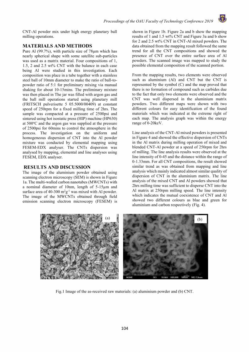
Proceedings of the OAU Faculty of Technology Conference 2019
104
CNT-Al powder mix under high energy planetary ball milling operations.
MATERIALS AND METHODS Pure Al (99.7%), with particle size of 78µm which has nearly spherical shape with some satellite sub-particles was used as a matrix material. Four compositions of 1, 1.5, 2 and 2.5 wt% CNT with the balance in each case being Al were studied in this investigation. Each composition was place in a tube together with a stainless steel ball of 10mm diameter to make the ratio of ball-to-powder ratio of 5:1 for preliminary mixing via manual shaking for about 10-15mins. The preliminary mixture was then placed in The jar was filled with argon gas and the ball mill operations started using planetary mill (FRITSCH pulverisette 5 05.5000/00409) at constant speed of 250rpm for a fixed milling time of 2hrs. The sample was compacted at a pressure of 2500psi and sintered using hot isostatic press (HIP) machine (HP630) at 500oC and the argon gas was supplied at the pressure of 2500psi for 60mins to control the atmosphere in the process. The investigation on the uniform and homogeneous dispersion of CNT into the Al powder mixture was conducted by elemental mapping using FESEM-EDX analyser. The CNTs dispersion was analysed by mapping, elemental and line analyses using FESEM, EDX analyser. RESULTS AND DISCUSSION The image of the aluminium powder obtained using scanning electron microscopy (SEM) is shown in Figure 1a. The multi-walled carbon nanotubes (MWCNTs) with a nominal diameter of 10nm, length of 5-15µm and surface area of 40-300 m2g-1 was mixed with Al powder. The image of the MWCNTs obtained through field emission scanning electron microscopy (FESEM) is
shown in Figure 1b. Figure 2a and b show the mapping results of 1 and 1.5 wt% CNT and Figure 3a and b show for 2 and 2.5 wt% CNT in CNT-Al mixed powders. The data obtained from the mapping result followed the same trend for all the CNT compositions and showed the presence of CNT over the entire surface area of Al powders. The scanned image was mapped to study the possible elemental composition of the scanned portion. From the mapping results, two elements were observed such as aluminium (Al) and CNT but the CNT is represented by the symbol (C) and the map proved that there is no formation of compound such as carbides due to the fact that only two elements were observed and the CNT was well dispersed in the aluminium matrix powders. Two different maps were shown with two different colours for easy identification of the found materials which was indicated at the extreme right of each map. The analysis graph was within the energy range of 0-20keV. Line analysis of the CNT-Al mixed powders is presented in Figure 4 and showed the effective dispersion of CNTs in the Al matrix during milling operation of mixed and blended CNT-Al powder at a speed of 250rpm for 2hrs of milling. The line analysis results were observed at the line intensity of 0-45 and the distance within the range of 0-1.33mm. For all CNT compositions, the result showed similar trend as was obtained from mapping and line analysis which mainly indicated almost similar quality of dispersion of CNT in the aluminium matrix. The line analysis of the mixed CNT and Al powders showed that 2hrs milling time was sufficient to disperse CNT into the Al matrix at 250rpm milling speed. The line intensity which indicates the mutual coexistence of CNT and Al showed two different colours as blue and green for aluminium and carbon respectively (Fig. 4).
Fig.1 Image of the as-received raw materials: (a) aluminium powder and (b) CNT.
(a) (b)
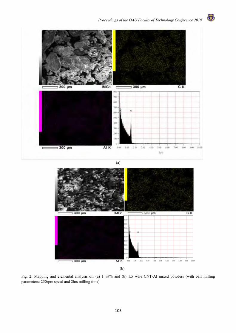
Proceedings of the OAU Faculty of Technology Conference 2019
105
(a)
Fig. 2: Mapping and elemental analysis of: (a) 1 wt% and (b) 1.5 wt% CNT-Al mixed powders (with ball milling parameters: 250rpm speed and 2hrs milling time).
(b)
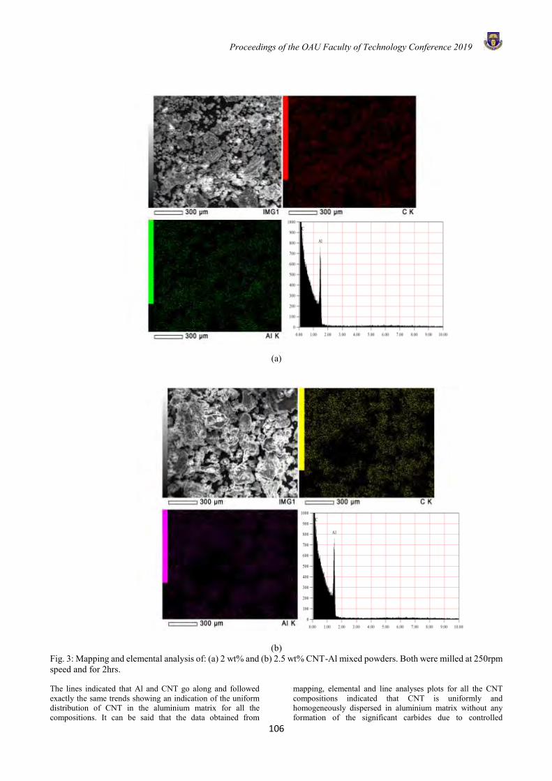
Proceedings of the OAU Faculty of Technology Conference 2019
106
(a)
(b)
Fig. 3: Mapping and elemental analysis of: (a) 2 wt% and (b) 2.5 wt% CNT-Al mixed powders. Both were milled at 250rpm speed and for 2hrs.
The lines indicated that Al and CNT go along and followed exactly the same trends showing an indication of the uniform distribution of CNT in the aluminium matrix for all the compositions. It can be said that the data obtained from
mapping, elemental and line analyses plots for all the CNT compositions indicated that CNT is uniformly and homogeneously dispersed in aluminium matrix without any formation of the significant carbides due to controlled
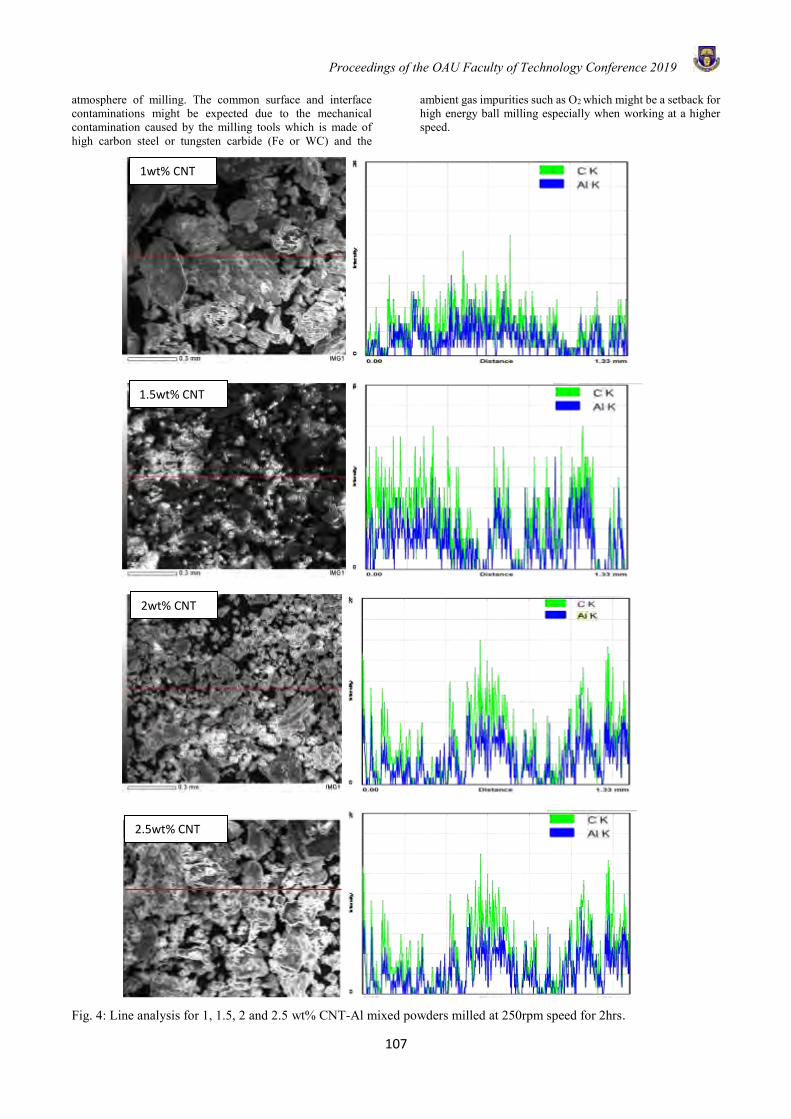
Proceedings of the OAU Faculty of Technology Conference 2019
107
atmosphere of milling. The common surface and interface contaminations might be expected due to the mechanical contamination caused by the milling tools which is made of high carbon steel or tungsten carbide (Fe or WC) and the
ambient gas impurities such as O2 which might be a setback for high energy ball milling especially when working at a higher speed.
Fig. 4: Line analysis for 1, 1.5, 2 and 2.5 wt% CNT-Al mixed powders milled at 250rpm speed for 2hrs.
1wt% CNT
1.5wt% CNT
2wt% CNT
2.5wt% CNT
Proceedings of the OAU Faculty of Technology Conference 2019
108
However, in this investigation, the involvement of argon gas during milling operation has eliminated all unwanted reactions that are likely to occur during the process and the use of suitable milling speed and time also helped in preventing the contamination. Therefore, the use of argon gas in milling operation is very vital as it controls surface and interface contamination which are likely to occur during the fabrication of any composite material via high energy ball milling, Esawi et al. [4]. CONCLUSION The characterisation of CNT dispersion in CNT-Al powder mix was successfully performed. The data obtained from mapping, elemental and line analyses plots of all the CNT compositions indicated that CNT is uniformly and homogeneously dispersed in aluminium powder without any formation of carbides due to the controlled atmosphere of milling. It can be concluded that the FESEM-EDX is a tool that can be used for the characterisation of CNT dispersion in CNT-Al powder mix before utilising this for the nano-composite development. ACKNOWLEDGEMENT The researchers acknowledged the management of International Islamic University Malaysia for utilising their equipments for all the experiment. REFERENCES Bakshi, S.R., D. Lahiri, and A. Agarwal, Carbon nanotube reinforced metal matrix composites‐a review. International Materials Reviews, 2010. 55(1): p.41-64. Iijima, S., Helical microtubules of graphitic carbon.
Nature, 1991. 354(6348): p.56-58. Javadi, A., S. Mirdamadi, M. Faghihisani, S. Shakhesi,
and R. Soltani, Fabrication of well-dispersed, multiwalled carbon nanotubes-reinforced aluminum matrix composites. New Carbon Materials, 2012. 27(3): p.161-165.
Maleque M.A, Abdullahi U. and M. Y. Ali (2015). Morphology of CNT-Al Nanocomposite Under Different Ball Milling Parameters, Advanced Materials Research, 1115 398-401
Mohammed Baba Ndaliman, Katsina Christopher Bala,
Ahsan Ali Kha, Mohammad Yeakub Ali, Umma Abdullahi and Adebisi Adetayo Abdulmumin (2015). The effects of Sliding Parameters on Dry Wear Characteristics of Ti-6Al-4V Alloy, Advanced Materials Research,1115 213-216.
Morsi, K. and A. Esawi, Effect of mechanical alloying time and carbon nanotube (CNT) content on the evolution of aluminum (Al)–CNT composite powders. Journal of materials science, 2007. 42(13): p. 4954-4959.
Morsi, K., A. Esawi, P. Borah, S. Lanka, A. Sayed, and M. Taher, Properties of single and dual matrix aluminum–carbon nanotube composites
processed via spark plasma extrusion (SPE). Materials Science and Engineering: A, 2010. 527(21): p. 5686-5690.
Poirier, D., R. Gauvin, and R.A. Drew, Structural characterisation of a mechanically milled carbon nanotube/aluminum mixture. Composites Part A: Applied Science and Manufacturing, 2009. 40(9): p.1482-1489.
Savage, G., Carbon-carbon composites. 1993: Kluwer Academic Publishers.
Sridhar, I. and K.R. Narayanan, Processing and characterization of MWCNT reinforced aluminum matrix composites. Journal of materials science, 2009. 44(7): p.1750-1756.
Umma, A., Maleque, M. A. and Ali, M. Y. (2018). Characterization of Carbon Nanotube Reinforced Aluminium Nanocomposite Using Field Emission Scanning Electron Microscope. International Journal of Engineering Materials and Manufacture, 3(1), 63-67.
Proceedings of the OAU Faculty of Technology Conference 2019
109
MODEL IDENTIFICATION OF BIOMASS BOILER SYSTEM USING PRINCIPAL COMPONENT REGRESSION
T. A. Morakinyo*1 and C. T. Akanbi1 1Department of Food Science and Technology Obafemi Awolowo University, Ile-Ife, Nigeria.
*Email of Corresponding Author: [email protected]
ABSTRACT The focus of this study was to identify boiler operational variables that positively and negatively contributed to the boiler biomass utility using Principal Component Regression (PCR) to enhance its thermal efficiency. An installed biomass fired vertical boiler was developed and evaluated by combusting 30.0 kg of charcoal to generate superheated steam within 3.0 hrs. Biomass utility was chosen as independent variable while steam pressure, steam chamber temperature, superheat steam flow rate, exhaust gas temperature, inner and outer insulated wall temperatures were dependent variables. Experimental data obtained were recorded values of dependent variables against independent at an interval of 10 minutes. The factor analysis of Biplot model was adopted to categorise the variables into two; hence factor loading was validated using STATISTICAL 12 factor analysis model. The correlation between variables and factors was established to determine the level of significance and validated using squared cosines and percentage of contribution of each variable. The result showed that the coefficient of determinations of both factors analyses using principal component regression model fit the measured responses at levels of 99.40% and 95.07%, respectively. The principal component regression model indicated that superheated steam flow rate and steam pressure contributed positively while steam chamber temperature, exhaust gas temperature, inner and outer insulated wall temperatures contributed negatively to biomass utility. This indicated that the rest of the system variables apart from the steam pressure and the superheated steam flow rate reduce biomass utility which increases the cost of operation of the newly developed boiler. Conclusively, the variables required further modification had been identified to eradicate heat losses and enhance thermal efficiency.
Keywords: Operational boiler variables, Principal component regression models, Greenhouse gases, Biomass fired boiler, Steam generation.
INTRODUCTION The development and further modifications of indigenous steam generators of various capacities is required in Africa for economic and industrial emancipation. In the United State of America, about 1.3 million of boilers of different types and capacities were installed and monitored at industrial, commercial and institutional settings for further modifications (Panel, 2009). Boiler is the major unit operation in any power generation turbine plant. However, poor thermal efficiency and inefficient energy conservation in boiler design will increase its running cost and generate greenhouse gases that support global warming (Oyedepo, 2012). The generated steam has wider applications that cover about 35-40% of energy usage in industry globally (UNIDO, 2016). These applications are energy conversion systems, food processes and production support in confectionary, brewery, sugar, salt, oilseeds, dairy, paper, petroleum, chemicals, plastics, rubber, textile, pharmaceuticals, and refining and primary metals industries. Furthermore, other areas of steam applications are: heat and mass transfer process (drying, blanching, hermetical sterilization and separation), power generation plants, water treatment, cleaning in place (CIP) of the units operation, packaging (gum melting), storage, waste management, heating of buildings, dry cleaners and laundries (UNIDO, 2016).
Hence, the advantages of steam utilization in industry cannot be over emphasized due to some peculiar characteristics such as: constant temperature, high heat transfer coefficient, highest latent heat per unit mass, and extremely cost effective and high flexible energy transfer factor (Lienhard and Lienhard, 2017). Over decades, different types of steam generator, commonly referred to as boiler had been developed to suit aforementioned purposes. The industrial boiler can be classified into two namely: water-in-tube and fire-in-tube (Master et al., 2003; Yang et al., 2018; Morakinyo and Bamgboye, 2016). Previous researchers reported that biomass has potential for energy generation due to its availability at low price, renewable energy source coupled with carbon neutral features (Ojolo et al., 2012; Orisalaye et al., 2018).
The efficiency of any boiler can be rated on how effective its net input thermal energy can be converted optimally to thermal energy output (Reddy and Reddy, 2013). It has also been reported that the economical operation of any boiler depends on its thermal efficiency rating (Wang et al., 2014). Several factors that contributed to this efficiency are: boiler variables, accessories status, types of fuel and moisture content value, level of scaling and climatic conditions, optimum stoichiometric fuel and air ratio, adequate maintenance of heat transfer surfaces,
Proceedings of the OAU Faculty of Technology Conference 2019
110
installation of heat recovery equipment, add or replace boiler refractory effectively, standardizing and regular calibration of fuel (Shah and Adhyaru, 2011; Wang et al., 2014; UNIDO, 2016). There are various areas of energy efficiency sustenance and conservation studies in boiler operation management which were reported by previous researchers (Heikki, 2014; UNIDO, 2016). Other researchers (Wang et al., 2014) adopted principal component analysis model to improve the thermal efficiency of an industrial boiler online and estimated the key influential parameters for operator adjustment. It was reported by Yang et al. (2018) that effective biomass utility, combustion, heat transfer efficiency, adequate energy conversion, avoidable energy losses, high auxiliary power consumption, water quality, environmental pollution and excessive production of flue gases as factors militating against optimum thermal efficiency among others. The reported studies (Heikki, 2014; Febrero et al., 2015) on biomass boiler emission characterization and control include the influence of combustion parameters on fouling composition and its effect on thermal efficiency. But the effect of dependent variables on the consumption rate of the biomass of a laboratory-scale boiler is yet to be reported. A newly developed and installed biomass fire-in-tube boiler was evaluated to identify among the operational parameters which ones are positively or negatively influencing biomass utility. This work also seeks to develop a model for this boiler using Principal Component Regression (PCR) model for a training data set obtained and validated using historical data from the system. Hence, this study objective of this work is to identify those boiler variables that are of positive and negative influence for further modification on this newly developed fire-in-tube biomass fired boiler for further modifications, optimum thermal efficiency, economical purpose, and environmental pollution control.
Theory of PCR Model for the Biomass Utility
Principal Components Regression (PCR) is a technique for analysing multiple regression data that suffer from multi-colinearity (NCSS, 2018). This gives a lot of advantages over Multiple Linear Regression models. Principal Components Analysis (PCA) from which PCR was developed and it is found to cope well with data that is noisy, and with situations where the data is sparse or rather when there is little data relative to the number of inputs being regressed. Ideally, PCR reduces the number of variables monitored which are correlated while retaining as much of the variability contained in the original data as possible.
MATERIALS AND METHODS
A newly developed and installed biomass-fired fire-in-tube insulated vertical boiler at Department of Food Science and Technology, Obafemi Awolowo University, Ile-Ife, Osun State, Nigeria was evaluated to identify operational parameters that will enhance its thermal efficiency or not. This boiler consists of combustion chamber, fire deflector, kettle, steam chamber, insulated body, frame, chimney, pressure relief valve, thermometer and pressure gauge. The total dimension of the vertical boiler is Ø 500 × 1050 mm vertical height with insulated wall of 50 mm thickness on both combustion chamber and kettle (Plate 1). At the combustion chamber, the vertical height of the fire grate to the bottom of the kettle was predetermined and adjusted to 280 mm while orifice area of the chimney was kept at 2 dm2 in correlation to the optimum values reported by Morakinyo and Bamgboye, 2017.
The boiler was evaluated by loading the combustion chamber with 30.0 kg of charcoal for a period of 3.0 hours gradually to generate superheated steam. At the beginning of the experiment, the kettle of the boiler was fed manually with 60 litres of water through an inlet port and all gate valves were locked to create closed system (Plate 1). A steam collector was coupled to the main steam discharge gate valve via a T-connector to measure the steam flow rate at 10 minutes interval. The flow rate at each interval was determined by discharging superheated steam into the steam collector through the main discharge gate valve in a minute. At the bottom of the steam collector, another gate valve was fitted to retain the steam to collect condensate. The condensate obtained at each interval was discharged into a measuring cylinder to measure the volume for measuring. Thermocouples were installed at the chimney, steam chamber wall, inner insulated wall and outer insulated wall, to obtain exhaust gas temperature and walls temperature, respectively. While temperature logger in range of 0-300 oC was used to obtained thermocouple temperature values. Then all the gate valves were closed while charcoal was ignited to generate heat energy gradually. The experimental data was obtained by recording values of temperature and pressure of superheated steam generated through thermometer and pressure gauge installed on top of the steam chamber of the boiler, and temperatures of others at an interval of 10 minutes for 3.0 hrs. The maximum temperature and pressure values obtained at the end of the experiment were, 10 bar pressure and 200 oC temperature, having a steam generated capacity of 40 litres/hr. The system variables are shown in Table 1 with their respective unit.

Proceedings of the OAU Faculty of Technology Conference 2019
111
Plate 1: Fire-in-tube biomass fired vertical boiler
Table 1: System Variables (Identification tools).
Measuring point Unit
Time S Steam chamber temperature Steam pressure Bar Biomass Utility MJ/kg Insulated inner wall temperature Insulated outer wall temperature Flue gases temperature at chimney Superheated steam flow rate cm3/s
Data Analysis
PCA was adopted for data analysis because of the high correlations that exist among the boiler variables. Biomass utility was selected as dependent variable while others were dependent variables (Table 1). The XLSTAT was adopted using Bioplot models through factor analysis to categorize the dependent variables into two; hence factor loading was validated using STATISTICAL 12 factor analysis model. The correlation between variables and factors was established to determine the level of significance and validated using squared cosines and percentage of contribution of each variable. The correlation matrix shown the level of interaction of principal components against each other at a significance level of alpha is 0.05.
RESULTS AND DISCUSSIONS
Factor analysis on experimental data was adopted to categorise the dependent variables into two groups using Biplot models. In Figure 1, Biplot model showed quadratic curve which categorized system dependent variables across the four quadrants having Biplot axes F1 and F2 for X and Y axes, respectively. Those dependent variables that were categorized along axis of F2 negative coordinate were: Steam Chamber Temperature (SCT), Exhaust Gas Temperature (EGT), Insulated Outer Wall Temperature (IWTO) and Insulated Inner Wall Temperature (IWTI). Likewise those independent variable categorized along axis of F2 positive coordinate were: Super Heated Steam Flow Rate (SHSFR) and Steam Pressure (P) as also depicted in Figure 1.
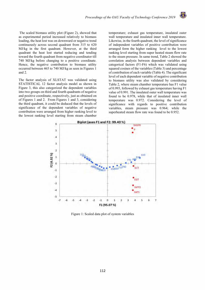
Proceedings of the OAU Faculty of Technology Conference 2019
112
The scaled biomass utility plot (Figure 2), showed that as experimental period increased relatively to biomass loading, the heat lost was on downward or negative trend continuously across second quadrant from 315 to 620 MJ/kg in the first quadrant. However, at the third quadrant the heat lost started reducing and tending toward the fourth quadrant from negative coordinator till 740 MJ/kg before changing to a positive coordinate. Hence, the negative contribution to biomass utility occurred between 465 to 740 MJ/kg as seen in Figures 1 and 2.
The factor analysis of XLSTAT was validated using STATISTICAL 12 factor analysis model as shown in Figure 3, this also categorized the dependent variables into two groups on third and fourth quadrants of negative and positive coordinate, respectively, just as obtained on of Figures 1 and 2. From Figures 1 and 3, considering the third quadrant, it could be deduced that the levels of significance of the dependent variables of negative contribution were arranged from higher ranking level to the lowest ranking level starting from steam chamber
temperature; exhaust gas temperature, insulated outer wall temperature and insulated inner wall temperature. Likewise, in the fourth quadrant, the level of significance of independent variables of positive contribution were arranged form the higher ranking level to the lowest ranking level starting from super heated steam flow rate to the steam pressure. In same trend, Table 2 showed the correlation analysis between dependent variables and categorical factors (F1-F6) which was validated using squared cosines of the variables (Table 3) and percentage of contribution of each variable (Table 4). The significant level of each dependent variable of negative contribution to biomass utility was also validated by considering Table 2, where steam chamber temperature has F1 value of 0.993, followed by exhaust gas temperature having F1 value of 0.991. The insulated outer wall temperature was found to be 0.978, while that of insulated inner wall temperature was 0.972. Considering the level of significance with regards to positive contribution variables, steam pressure was 0.964; while the superheated steam flow rate was found to be 0.952.
Figure 1: Scaled data plot of system variables
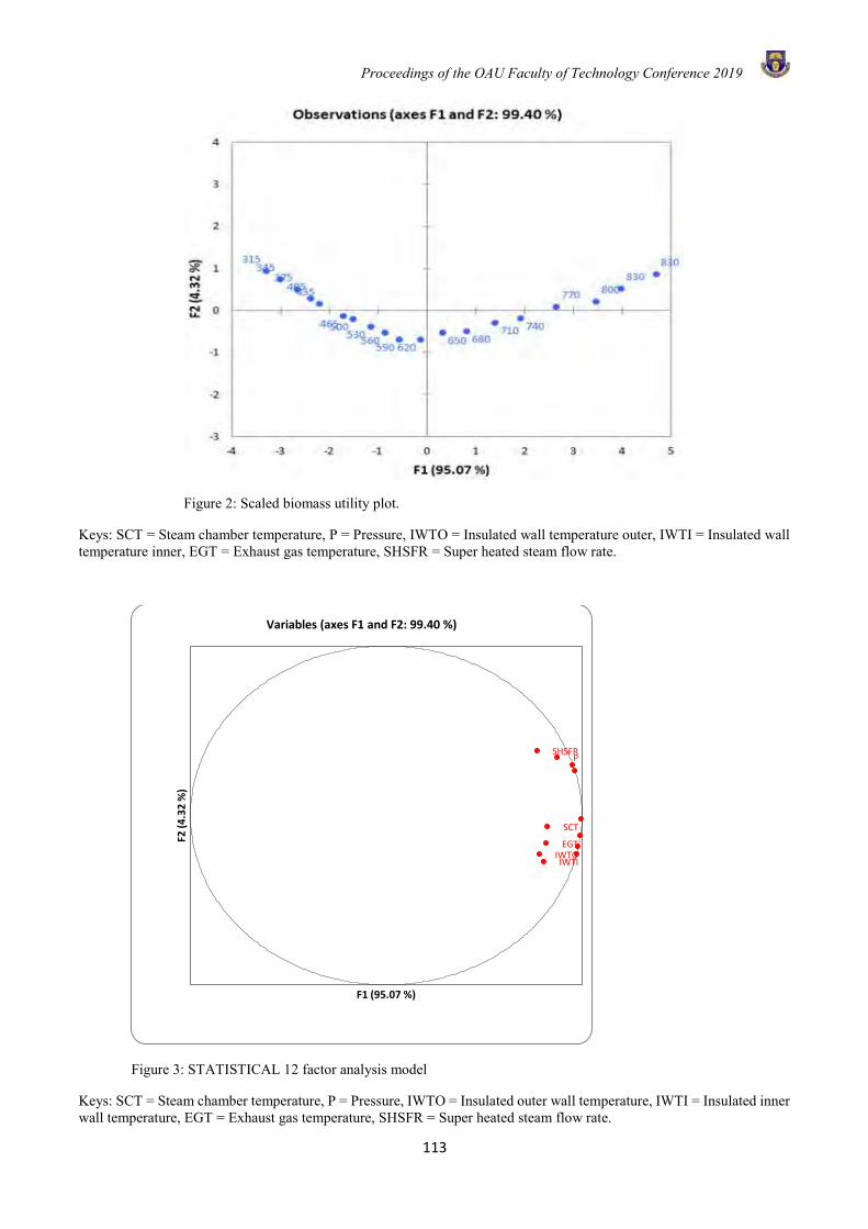
Proceedings of the OAU Faculty of Technology Conference 2019
113
Figure 2: Scaled biomass utility plot.
Keys: SCT = Steam chamber temperature, P = Pressure, IWTO = Insulated wall temperature outer, IWTI = Insulated wall temperature inner, EGT = Exhaust gas temperature, SHSFR = Super heated steam flow rate.
Figure 3: STATISTICAL 12 factor analysis model
Keys: SCT = Steam chamber temperature, P = Pressure, IWTO = Insulated outer wall temperature, IWTI = Insulated inner wall temperature, EGT = Exhaust gas temperature, SHSFR = Super heated steam flow rate.
SCT
P
IWTOIWTI
EGT
SHSFR
F2 (
4.3
2 %
)
F1 (95.07 %)
Variables (axes F1 and F2: 99.40 %)
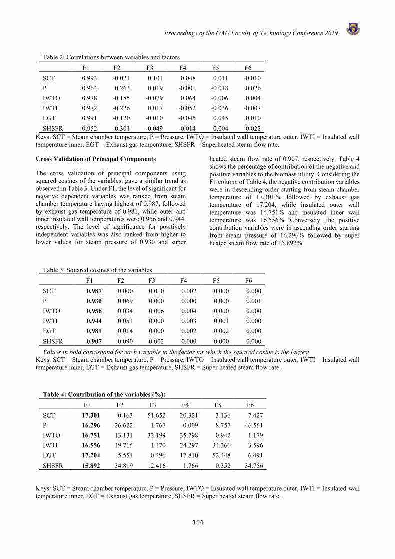
Proceedings of the OAU Faculty of Technology Conference 2019
114
Table 2: Correlations between variables and factors
F1 F2 F3 F4 F5 F6 SCT 0.993 -0.021 0.101 0.048 0.011 -0.010 P 0.964 0.263 0.019 -0.001 -0.018 0.026 IWTO 0.978 -0.185 -0.079 0.064 -0.006 0.004 IWTI 0.972 -0.226 0.017 -0.052 -0.036 -0.007 EGT 0.991 -0.120 -0.010 -0.045 0.045 0.010 SHSFR 0.952 0.301 -0.049 -0.014 0.004 -0.022
Keys: SCT = Steam chamber temperature, P = Pressure, IWTO = Insulated wall temperature outer, IWTI = Insulated wall temperature inner, EGT = Exhaust gas temperature, SHSFR = Superheated steam flow rate.
Cross Validation of Principal Components
The cross validation of principal components using squared cosines of the variables, gave a similar trend as observed in Table 3. Under F1, the level of significant for negative dependent variables was ranked from steam chamber temperature having highest of 0.987, followed by exhaust gas temperature of 0.981, while outer and inner insulated wall temperatures were 0.956 and 0.944, respectively. The level of significance for positively independent variables was also ranked from higher to lower values for steam pressure of 0.930 and super
heated steam flow rate of 0.907, respectively. Table 4 shows the percentage of contribution of the negative and positive variables to the biomass utility. Considering the F1 column of Table 4, the negative contribution variables were in descending order starting from steam chamber temperature of 17.301%, followed by exhaust gas temperature of 17.204, while insulated outer wall temperature was 16.751% and insulated inner wall temperature was 16.556%. Conversely, the positive contribution variables were in ascending order starting from steam pressure of 16.296% followed by super heated steam flow rate of 15.892%.
Table 3: Squared cosines of the variables
F1 F2 F3 F4 F5 F6 SCT 0.987 0.000 0.010 0.002 0.000 0.000 P 0.930 0.069 0.000 0.000 0.000 0.001 IWTO 0.956 0.034 0.006 0.004 0.000 0.000 IWTI 0.944 0.051 0.000 0.003 0.001 0.000 EGT 0.981 0.014 0.000 0.002 0.002 0.000 SHSFR 0.907 0.090 0.002 0.000 0.000 0.000 Values in bold correspond for each variable to the factor for which the squared cosine is the largest
Keys: SCT = Steam chamber temperature, P = Pressure, IWTO = Insulated wall temperature outer, IWTI = Insulated wall temperature inner, EGT = Exhaust gas temperature, SHSFR = Super heated steam flow rate.
Table 4: Contribution of the variables (%):
F1 F2 F3 F4 F5 F6 SCT 17.301 0.163 51.652 20.321 3.136 7.427 P 16.296 26.622 1.767 0.009 8.757 46.551 IWTO 16.751 13.131 32.199 35.798 0.942 1.179 IWTI 16.556 19.715 1.470 24.297 34.366 3.596 EGT 17.204 5.551 0.496 17.810 52.448 6.491 SHSFR 15.892 34.819 12.416 1.766 0.352 34.756
Keys: SCT = Steam chamber temperature, P = Pressure, IWTO = Insulated wall temperature outer, IWTI = Insulated wall temperature inner, EGT = Exhaust gas temperature, SHSFR = Super heated steam flow rate.
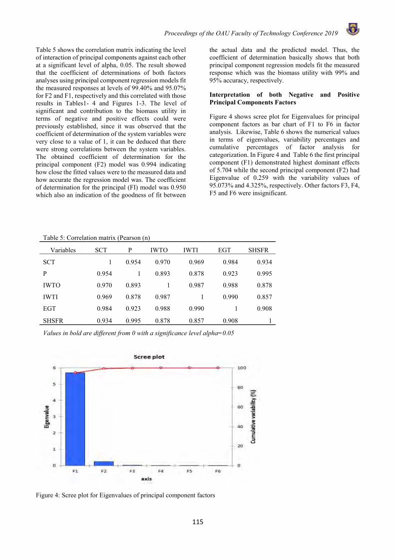
Proceedings of the OAU Faculty of Technology Conference 2019
115
Table 5 shows the correlation matrix indicating the level of interaction of principal components against each other at a significant level of alpha, 0.05. The result showed that the coefficient of determinations of both factors analyses using principal component regression models fit the measured responses at levels of 99.40% and 95.07% for F2 and F1, respectively and this correlated with those results in Tables1- 4 and Figures 1-3. The level of significant and contribution to the biomass utility in terms of negative and positive effects could were previously established, since it was observed that the coefficient of determination of the system variables were very close to a value of 1, it can be deduced that there were strong correlations between the system variables. The obtained coefficient of determination for the principal component (F2) model was 0.994 indicating how close the fitted values were to the measured data and how accurate the regression model was. The coefficient of determination for the principal (FI) model was 0.950 which also an indication of the goodness of fit between
the actual data and the predicted model. Thus, the coefficient of determination basically shows that both principal component regression models fit the measured response which was the biomass utility with 99% and 95% accuracy, respectively.
Interpretation of both Negative and Positive Principal Components Factors
Figure 4 shows scree plot for Eigenvalues for principal component factors as bar chart of F1 to F6 in factor analysis. Likewise, Table 6 shows the numerical values in terms of eigenvalues, variability percentages and cumulative percentages of factor analysis for categorization. In Figure 4 and Table 6 the first principal component (F1) demonstrated highest dominant effects of 5.704 while the second principal component (F2) had Eigenvalue of 0.259 with the variability values of 95.073% and 4.325%, respectively. Other factors F3, F4, F5 and F6 were insignificant.
Table 5: Correlation matrix (Pearson (n)
Variables SCT P IWTO IWTI EGT SHSFR
SCT 1 0.954 0.970 0.969 0.984 0.934
P 0.954 1 0.893 0.878 0.923 0.995
IWTO 0.970 0.893 1 0.987 0.988 0.878
IWTI 0.969 0.878 0.987 1 0.990 0.857
EGT 0.984 0.923 0.988 0.990 1 0.908
SHSFR 0.934 0.995 0.878 0.857 0.908 1
Values in bold are different from 0 with a significance level alpha=0.05
Figure 4: Scree plot for Eigenvalues of principal component factors
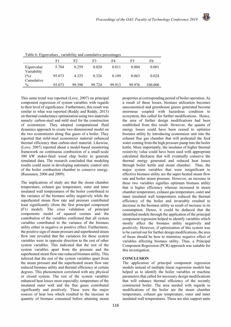
Proceedings of the OAU Faculty of Technology Conference 2019
116
Table 6: Eigenvalues , variability and cumulative percentages F1 F2 F3 F4 F5 F6
Eigenvalue 5.704 0.259 0.020 0.011 0.004 0.001 Variability (%) 95.073 4.325 0.326 0.189 0.063 0.024 Cumulative % 95.073 99.398 99.724 99.913 99.976 100.000
This same trend was reported (Love, 2007) on principal component regression of system variables with regards to their level of significance. Furthermore, this result was similar to what was reported (Reddy and Reddy, 2013) on thermal conductance optimization using two materials namely: carbon-steel and mild steel for the construction of economizer. They adopted computational fluid dynamics approach to create two-dimensional model on the two economizers along flue gases of a boiler. They reported that mild-steel economizer material enhanced thermal efficiency than carbon-steel material. Likewise, (Love, 2007) reported about a model-based monitoring framework on continuous combustion of a small-scale 300 kW stoker-fired wood chip boiler to generate simulated data. The research concluded that modeling results could assist in developing automatic control unit of the boiler combustion chamber to conserve energy. (Ruusunen, 2006 and 2009).
The implications of study are that the steam chamber temperature, exhaust gas temperature, outer and inner insulated wall temperatures of the boiler contributed to the variance of the biomass utility negatively while the superheated steam flow rate and pressure contributed least significantly (from the first principal component (F1) model). The cross validation of principal components model of squared cosines and the contribution of the variables confirmed that all system variables contributed to the variance of the biomass utility either in negative or positive effect. Furthermore, the positive sign of steam pressure and superheated steam flow rate revealed that the variances for these system variables were in opposite direction to the rest of other system variables. This indicated that the rest of the system variables apart from the pressure and the superheated steam flow rate reduced biomass utility. This inferred that the rest of the system variables apart from the steam pressure and the superheated steam flow rate reduced biomass utility and thermal efficiency at certain degrees. This phenomenon correlated with any physical or closed system. The rest of the system variables enhanced heat losses most especially; temperature of the insulated outer wall and the flue gases contributed significantly and positively. These were the major sources of heat loss which resulted to the increase in quantity of biomass consumed before attaining steam
properties at corresponding period of boiler operation. As a result of these losses, biomass utilization becomes uneconomical and greenhouse gasses generated become enormous coupled with hazardous condition to ecosystem, this called for further modifications. Hence, the area of further design modifications had been established from this result. However, the quanta of energy losses could have been reused to optimize biomass utility by introducing economizer unit into the exhaust flue gas chamber that will preheated the feed water coming from the high pressure pump into the boiler kettle. More importantly, the insulator of higher thermal resistivity value could have been used with appropriate calculated thickness that will eventually conserve the thermal energy generated and reduced heat losses through boiler kettle and steam chamber. Thus, the major system variables that were insignificant to effective biomass utility are the super-heated steam flow rate and boiler steam pressure. However, an increase in these two variables signifies optimum biomass utility that is higher efficiency whereas increased in steam chamber temperature, exhaust gas temperature, outer and inner insulated wall temperatures reduced the thermal efficiency of the boiler and invariably resulted to decrease in the biomass utility as result of increase in its consumption. Hence, it could be deduced that the identified models through the application of the principal component regression helped to identify variables which mostly affect the biomass utility negatively and positively. However, if optimization of this system was to be carried out for further design modifications, the area of focus should be how to minimize negative effect of variables affecting biomass utility. Thus, a Principal Component Regression (PCR) approach was suitable for this investigation.
CONCLUSION The application of principal component regression models instead of multiple linear regression models has helped us to identify the boiler variables or machine parameters that called for necessary design modifications that will enhance thermal efficiency of the recently constructed boiler. The area needed with regards to modifications of the boiler are the steam chamber temperature, exhaust gas temperature, outer and inner insulated wall temperatures. These are also support units
Proceedings of the OAU Faculty of Technology Conference 2019
117
to the process unit of the boiler that are in contact with the environment. This means that the whole boiler metallic structure should be housed with higher thermal resistivity insulator value for higher thermal efficiency. This can be accomplished by replacing the existing glass fibre with another insulator of higher thermal resistivity and employing appropriate design calculation to determine its optimum thickness. More importantly, an economizer should be introduced to preheat feed water before entering the kettle. Generally, steam generators should be re-calibrated on regular bases, likewise their thermal efficiency validated whether the lagging is efficient or otherwise. Empirically, from Table 4, the steam chamber temperature contributed negatively at higher percentage than other parameters, since there was no lagging material to conserve heat of conduction through outer wall of this chamber to the environment. Hence for further modification, appropriate insulation material and thickness should be installed to conserve heat content of the superheated steam generated. This will enhance positive biomass utility and eventually reduce cost of operation. Obviously, higher energy efficient system will ensure effective biomass utility. In the same trend, to reduce heat loss through flue gases, the permanent solution is to install an economizer that will pre-heat the feed water before entering into the kettle, thereby inhibiting heat losses which affect biomass utility negatively.
ACKNOWNLEGDEMENTS The authors wish to appreciate the facilities provided by the Department of Food Science and Technology, Faculty of Technology, Obafemi Awolowo University, Ile-Ife, Osun State, Nigeria toward the success of this research work.
REFERENCES Febrero, L., Granada, E., Regueiro, A., Míguez , J.L.
(2015). Influence of Combustion Parameters on Fouling Composition after Wood Pellet Burning in a Lab-Scale Low-Power Boiler Energies. 8, 9794-9816; doi:10.3390/en8099794.
Heikki, L. (2014). Small-scale pellet boiler emissions-characterization and comparison to other combustion unit. Academic Dissertation of Faculty of Science and Forestry of the University of Eastern Finland Kuopio,. Pg. 1-13.
https://www.epa.gov/sites/production/files/documents/20090210panelseroutreachmeeting.pdf Google Scholar.
Lienhard IV, J.H., Lienhard V, J.H. (2017). Heat transfer textbook. Fourth edition, Phlogiston press Cambridge Massachusetts, Version 2.1 pg. 10-34.
Love, J. (2007). Process Automation Handbook: A Guide to Theory and Practice. London: Springer London:.
Master, B.I. Chunangad KS, Pushpanathan V. (2003). Fouling mitigation using helix-changer heat exchangers. Proceedings of the ECI Conference
on Heat Exchanger Fouling and Cleaning: Fundamentals and Applications, Santa Fe, USA,317–322.
Morakinyo, T. A., Bamgboye , A. I. (2017). “The Optimization of Operational Parameters of a Biomass Fire-in-tube Boiler Using Taguchi Design Method.” American Journal of Food Science and Technology, vol. 5, no. 5 167-175. doi: 10.12691/ajfst-5-5-1.
Morakinyo, T.A., Bamgboye, A.I. (2016). Optimization of Operation Parameters of a vertical sterilizer of Medium-Scale Oil Palm Mill Using Taguchi Method, Journal of Food Process Engineering, 40(5) DOI: 10.1111/JFPE.12453.
NCSS.com. (2018). ‘Principal Components Regression’. Available at:https://ncss-wpengine.netdna-ssl.com/wp-content/themes/ncss/pdf/Procedures/NCSS/Principal_Components_Regression.pdf (Accessed: 10 July 2018),
Ojolo, S.J., Orisaleye, J.I., Ismail, S.O., Abolarin, S.M. (2012). Technical potential of biomass energy in Nigeria. Ife Journal of Technology, 21 (2):60–65.
Orisaleye, J.I., Jekayinfa, S.O., Adebayo, A.O., Ahmed, N.A., Pecenka, R. (2018). Effect of densification variables on density of corn cob briquettes produced using a uniaxial compaction biomass briquetting press, Energy Sources, Part A: Recovery, Utilization, and Environmental Effects, doi: 10.1080/15567036.2018.1516007.
Oyedepo, S.O. (2012). Energy Efficiency and Conservation Measures: Tools for Sustainable Energy Development in Nigeria. International Journal of Energy Engineering. IJEE, 2(3):86-98.
Panel, S. E.R. (2009). Outreach Meeting, Combined Rulemaking for Industrial, Commercial, and Institutional Boilers and Process Heaters at Major Sources of HAP and Industrial Boilers and Commercial and Institutional Boilers at Area Sources. https://www.epa.gov/sites/production/files/documents/20090210panelseroutreachmeeting.pdf Google Scholar
Reddy, K.S.K., Reddy, B.V. (2013). Performance of boiler and to improving the boiler efficiency using Cfd Modeling. Journal of Mechanical and Civil Engineering, 8(6): 25-29.
Ruusunen, M. (2006a). Monitoring of small-scale biomass combustion processes. Report Series A 29. March 2006. Department of Process and Environmental Engineering, Control Engineering Laboratory. ISBN 951-42-8027-X. ISSN 1238-9390 FIN-90014, University of Oulu,. Finland: 1-34.
Ruusunen, M. (2009). Modelling and control of small-scale biomass combustion for emission reduction. In: Paukkeri, A.; Ylä-Mella, J. and Pongrácz, E. (eds.) Energy research at the University of Oulu. Proceedings of the EnePro conference, June 3rd, 2009, University of Oulu,

Proceedings of the OAU Faculty of Technology Conference 2019
118
Finland. Kaleva print, Oulu,. ISBN 978-951-42-9154-8: 75-78.
Shah, S., Adhyaru, D.M. (2010). Boiler Efficiency Analysis using Direct Method. In: International Conference on Current Trends in Technology,. . IEEE Press, New York. 1–5.
UNIDO. (2016). Manual for industrial steam systems assessment and optimization. https://www unido.org/site/SSO-manual-print-final-20161109-one-pgev2pdf,.
Wang, W., Chen, L., Han, X., Ge, Z., Wang, S. (2014). Modelling and Application of Principal Component Analysis in Industrial Boiler. Advances in Neural Networks Springer International Publishing Switzerland,. 395–404. DOI: 10.1007/978-3-319-12436-0_44.
Yang, J. Oh, S.R., Liu, W. (2014). Optimization of shell and tube heat exchangers using a general design approach motivated by contractual theory. International Journal of heat and mass transfer, (77): 1144 -1154.
Proceedings of the OAU Faculty of Technology Conference 2019
119
THE INFLUENCE OF QUENCHING MEDIA ON HARDNESS AND TENSILE PROPERTIES OF AGE-HARDENED 7075 ALUMINIUM ALLOY
A. T. Abdulazeez1, D. M. Akinwumi1, D. A. Isadare1*, K. J. Akinluwade2, A. A. Daniyan1, T. O. Taiwo3, F. I. Alo1, A. R. Adetunji1, and M. O. Adeoye1
1Department of Materials Science and Engineering, Faculty of Technology, Obafemi Awolowo University, Ile-Ife 220005, Nigeria.
2Department of Research and Development, Prototype Engineering Development Institute, National Agency for Science and Engineering Infrastructure (NASENI), Ilesa 233036, Nigeria.
3Department of Mechanical Engineering, Faculty of Technology, Obafemi Awolowo University, Ile-Ife 220005, Nigeria.
*Email of Corresponding Author: [email protected]
ABSTRACT This paper investigated the influence of quenching media on the ageing response of 7075 aluminium alloy with a view of mitigating against the inherent deleterious effects of residual stress associated with convectional water quenching, thereby improving the mechanical properties of the alloy for automobile and aerospace applications. Standard tensile samples were subjected to solution heat treatment at 470 oC, soaked for 4 hours and then quenched in oil, water and brine. The quenched samples were then artificially aged at 180 oC and soaked for 1, 2, 3, 4 and 5 hours, followed by air cooling. After ageing, the as-received and heat treated samples were characterized using instron electromechanical testing machine, micro hardness tester and scanning electron microscope (SEM) equipped with energy dispersive spectroscope (EDS). The results obtained showed an increased in tensile strength and hardness with ageing time for all the three quenching media. Also, tensile strength and hardness increases across various quenching media in accordance with severity of the quenching media. The samples quenched in brine have the best strength and hardness (742 MPa and 231 VHN at 5 hours soaking time) and for other soaking times considered, followed by water (681 MPa and 215 VHN at 5 hours soaking time) and oil (623 MPa and 191 VHN at 5 hours soaking time). The reverse is the case for ductility as indicated by percentage elongation. The SEM/EDS of the microstructure also showed the morphology of the presence of phases (MgZn2, CuAl2, Mg2Si, etc.) in the matrix of the alloy which are more pronounced in those samples quenched in brine. Therefore, the research concluded that oil, water and brine are suitable quenching media for 7075 Al alloy. However, the best result was obtained with brine; which showed the highest tensile strength and hardness with marginal decrease in ductility for the holding time considered. Key words: Quenching media, age-hardened, 7075 Aluminium alloy, aging and severity. INTRODUCTION One of the major requirements of an alloy to be age-hardenable is its ability to develop supersaturated solid solution (SSS) by quenching from solution heat treatment temperature (Rajan et al., 2012). When aluminium alloy is solution heat treated at elevated temperatures, alloying elements are re-dissolved to produce a solute rich solid solution known as supersaturated solid solution. The objective of the solution treatment is to maximize the concentration of hardening alloying elements such as copper, zinc, magnesium, and silicon in the solid solution. The concentration and rate of dissolution of these elements increases with temperature, therefore, solution treatment temperatures are usually near the liquidus temperature of the alloy concern. If an alloy is slowly cooled from an elevated temperature, alloying elements are precipitated and diffuse from the solid solution to concentrate at the grain boundaries, small voids, undissolved particles, at dislocations, and
other imperfections in the aluminium lattice. To achieve optimal strength, toughness, and corrosion resistance, it is desirable to retard this diffusion process and keep the alloying elements in solid solution until the alloy is age hardened. Alloying elements are kept in solid solution in the matrix of base metal by quenching from the solution treatment temperature. After quenching, aluminium alloy is aged and during this process, a fine dispersion of alloying elements and compounds are precipitated that significantly increase the strength and hardness of the material (Isadare et al., 2015a; Croucher, 1982). Researchers have shown that excessively slow cooling allows excessive concentrations of alloying elements to develop on the grain boundaries which promote intergranular corrosion (Isadare et al., 2013). Therefore, it is important that cooling rates during quenching be sufficiently fast to minimize grain boundary precipitation (quench sensitivity) and ensure the development of SSS during quenching.
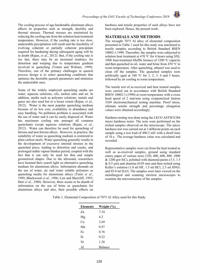
Proceedings of the OAU Faculty of Technology Conference 2019
120
The cooling process of age-hardenable aluminum alloys affects its properties such as strength, ductility and thermal stresses. Thermal stresses are minimized by reducing the cooling rate from the solution heat treatment temperature. However, if the cooling rate is too slow, undesirable precipitation will result and the feasibility of evolving coherent or partially coherent precipitate required for hardening during subsequent aging will be in doubt (Rajan, et al., 2012). But, if the cooling rate is too fast, there may be an increased tendency for distortion and warping due to temperature gradient involved in quenching (Totten and Webster, 1999). Therefore, one of the primary challenges in quench process design is to select quenching conditions that optimize the desirable quench parameters and minimize the undesirable ones. Some of the widely employed quenching media are water, aqueous solutions, oils, molten salts and air. In addition, media such as polymer solutions, metals and gases are also used but to a lesser extent (Rajan, et al., 2012). Water is the most popular quenching medium because of its low cost, availability in abundance and easy handling. No pollution problem is associated with the use of water and it can be easily disposed of. Water has maximum cooling rate amongst all common quenchants except aqueous solutions (Rajan, et al., 2012). Water can therefore be used for quenching of ferrous and non ferrous alloys. However, in practice, the suitability of water as quenching medium is restricted to plain carbon steels. Water quenching generally results in the development of excessive internal stresses in the quenched piece, leading to distortion and cracks, and prolonged stable vapour blanket period, coupled with the fact that it can only be used for thin and simple geometrical shapes. Due to the aforesaid, researchers have beamed their search light on alternative quenching medium for aluminium alloys. Information abounds on the use of water, air and water soluble polymers as quenching media for aluminium alloys (Tensi et al., 1999; Blackwood et al., 1996; Lim and Shercliff, 1993; Hart et al., 1980). However, there seems to be dearth of information on the use of brine as quenchants for aluminium alloys and also, their possible effects on
hardness and tensile properties of such alloys have not been explored. Hence, the present work. MATERIALS AND METHODS The wrought 7075 Al alloy of elemental composition presented in Table 1 used for this study was machined to tensile samples according to British Standard BSEN 10002-1:1990. Thereafter, the samples were subjected to solution heat treatment at 470 oC for 4 hours using SXL 1008 heat-treatment Muffle furnace of 1200 oC capacity and then quenched in oil, water and brine from 470 oC to room temperature. After quenching, ethanol was used to clean off the samples. The quenched samples were artificially aged at 180 °C for 1, 2, 3, 4 and 5 hours, followed by air cooling to room temperature. The tensile test of as-received and heat treated samples were carried out in accordance with British Standard BSEN 10002-1:(1990) at room temperature with a cross head speed of 2 mm/min using computerized Instron 3369 electromechanical testing machine. Proof stress, ultimate tensile strength and percentage elongation values were obtained accordingly. Hardness testing was done using the LECO ASTM E384 micro hardness tester. The tests were performed on the etched samples observed on the microscope. The micro hardness test was carried out at 3 different points on each sample using a test load of 490.3 mN with a dwell time of 10 s. The average hardness value was calculated and recorded. Representative samples were cut from the heat treated as well as as-received samples, ground using standard emery paper of various sizes (320, 400, 600, 800, 1000 & 1200 grit SiC), polished with diamond pastes (3.5, 1.5 & 0.5 μm) and alumina (0.05 nm) and then etched using Keller’s solution (1.0 ml HF, 1.5 ml HCl, 2.5 ml HNO3 and 95.0 ml H2O). The samples were later viewed on the metallurgical and scanning electron microscopes to examine the microstructure of the samples.
Table 1: Elemental Composition of 7075 Al Alloy used for this Study
Elements Weight (%) Zn 7.34 Mg 4.2 Cu 2.69 Mn 0.97 Fe 0.76 Si 0.22 Ni 1.28 Al Balance
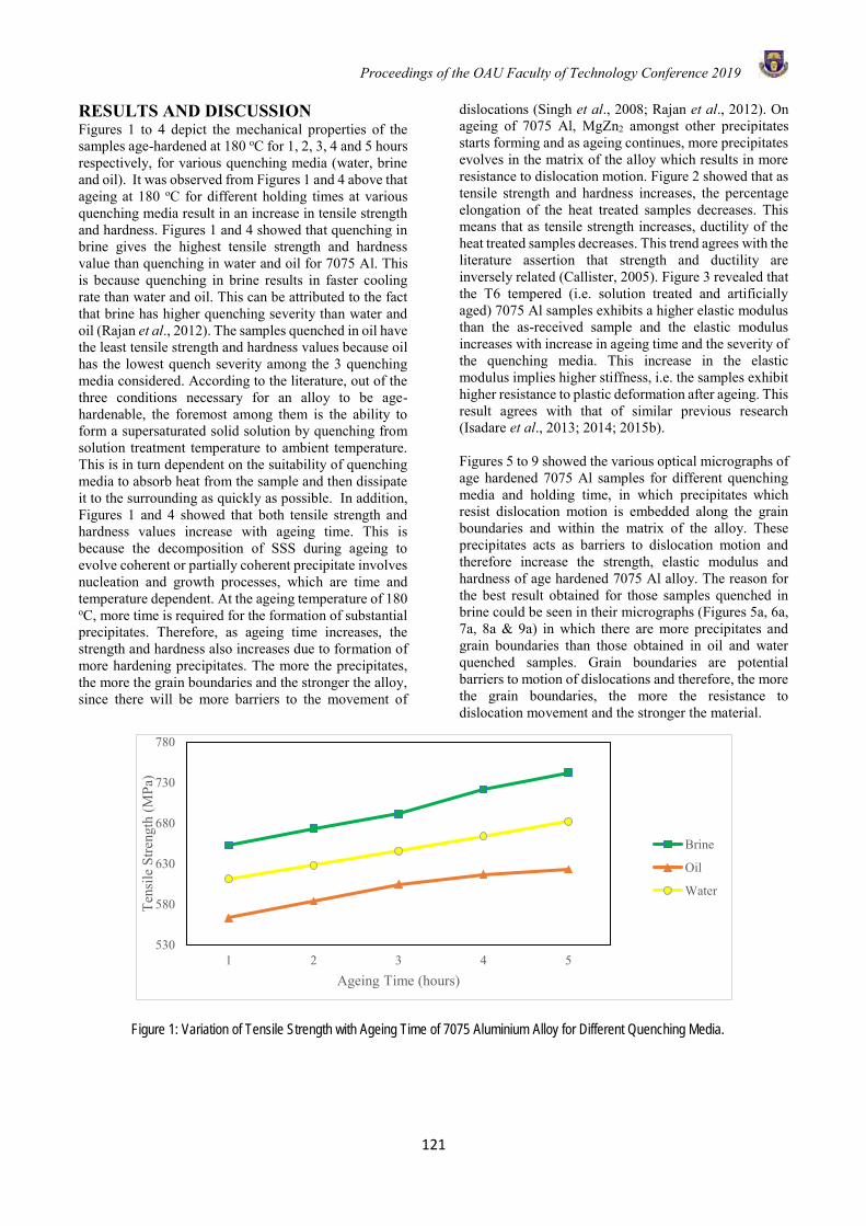
Proceedings of the OAU Faculty of Technology Conference 2019
121
RESULTS AND DISCUSSION Figures 1 to 4 depict the mechanical properties of the samples age-hardened at 180 oC for 1, 2, 3, 4 and 5 hours respectively, for various quenching media (water, brine and oil). It was observed from Figures 1 and 4 above that ageing at 180 oC for different holding times at various quenching media result in an increase in tensile strength and hardness. Figures 1 and 4 showed that quenching in brine gives the highest tensile strength and hardness value than quenching in water and oil for 7075 Al. This is because quenching in brine results in faster cooling rate than water and oil. This can be attributed to the fact that brine has higher quenching severity than water and oil (Rajan et al., 2012). The samples quenched in oil have the least tensile strength and hardness values because oil has the lowest quench severity among the 3 quenching media considered. According to the literature, out of the three conditions necessary for an alloy to be age-hardenable, the foremost among them is the ability to form a supersaturated solid solution by quenching from solution treatment temperature to ambient temperature. This is in turn dependent on the suitability of quenching media to absorb heat from the sample and then dissipate it to the surrounding as quickly as possible. In addition, Figures 1 and 4 showed that both tensile strength and hardness values increase with ageing time. This is because the decomposition of SSS during ageing to evolve coherent or partially coherent precipitate involves nucleation and growth processes, which are time and temperature dependent. At the ageing temperature of 180 oC, more time is required for the formation of substantial precipitates. Therefore, as ageing time increases, the strength and hardness also increases due to formation of more hardening precipitates. The more the precipitates, the more the grain boundaries and the stronger the alloy, since there will be more barriers to the movement of
dislocations (Singh et al., 2008; Rajan et al., 2012). On ageing of 7075 Al, MgZn2 amongst other precipitates starts forming and as ageing continues, more precipitates evolves in the matrix of the alloy which results in more resistance to dislocation motion. Figure 2 showed that as tensile strength and hardness increases, the percentage elongation of the heat treated samples decreases. This means that as tensile strength increases, ductility of the heat treated samples decreases. This trend agrees with the literature assertion that strength and ductility are inversely related (Callister, 2005). Figure 3 revealed that the T6 tempered (i.e. solution treated and artificially aged) 7075 Al samples exhibits a higher elastic modulus than the as-received sample and the elastic modulus increases with increase in ageing time and the severity of the quenching media. This increase in the elastic modulus implies higher stiffness, i.e. the samples exhibit higher resistance to plastic deformation after ageing. This result agrees with that of similar previous research (Isadare et al., 2013; 2014; 2015b). Figures 5 to 9 showed the various optical micrographs of age hardened 7075 Al samples for different quenching media and holding time, in which precipitates which resist dislocation motion is embedded along the grain boundaries and within the matrix of the alloy. These precipitates acts as barriers to dislocation motion and therefore increase the strength, elastic modulus and hardness of age hardened 7075 Al alloy. The reason for the best result obtained for those samples quenched in brine could be seen in their micrographs (Figures 5a, 6a, 7a, 8a & 9a) in which there are more precipitates and grain boundaries than those obtained in oil and water quenched samples. Grain boundaries are potential barriers to motion of dislocations and therefore, the more the grain boundaries, the more the resistance to dislocation movement and the stronger the material.
Figure 1: Variation of Tensile Strength with Ageing Time of 7075 Aluminium Alloy for Different Quenching Media.
530
580
630
680
730
780
1 2 3 4 5
Tens
ile S
treng
th (M
Pa)
Ageing Time (hours)
Brine
Oil
Water
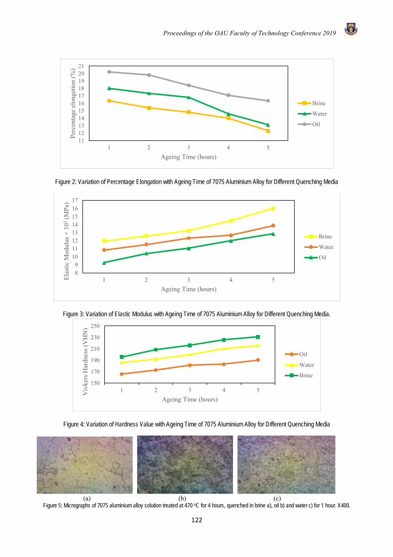
Proceedings of the OAU Faculty of Technology Conference 2019
122
Figure 2: Variation of Percentage Elongation with Ageing Time of 7075 Aluminium Alloy for Different Quenching Media
Figure 3: Variation of Elastic Modulus with Ageing Time of 7075 Aluminium Alloy for Different Quenching Media.
Figure 4: Variation of Hardness Value with Ageing Time of 7075 Aluminium Alloy for Different Quenching Media
(a) (b) (c)
Figure 5: Micrographs of 7075 aluminium alloy solution treated at 470 oC for 4 hours, quenched in brine a), oil b) and water c) for 1 hour. X400.
1112131415161718192021
1 2 3 4 5
Perc
enta
ge e
long
atio
n (%
)
Ageing Time (hours)
Brine
Water
Oil
89
1011121314151617
1 2 3 4 5Elas
tic M
odul
us ×
103
(MPa
)
Ageing Time (hours)
Brine
Water
Oil
150
170
190
210
230
250
1 2 3 4 5Viv
kers
Har
dnes
s (V
HN
)
Ageing Time (hours)
Oil
Water
Brine
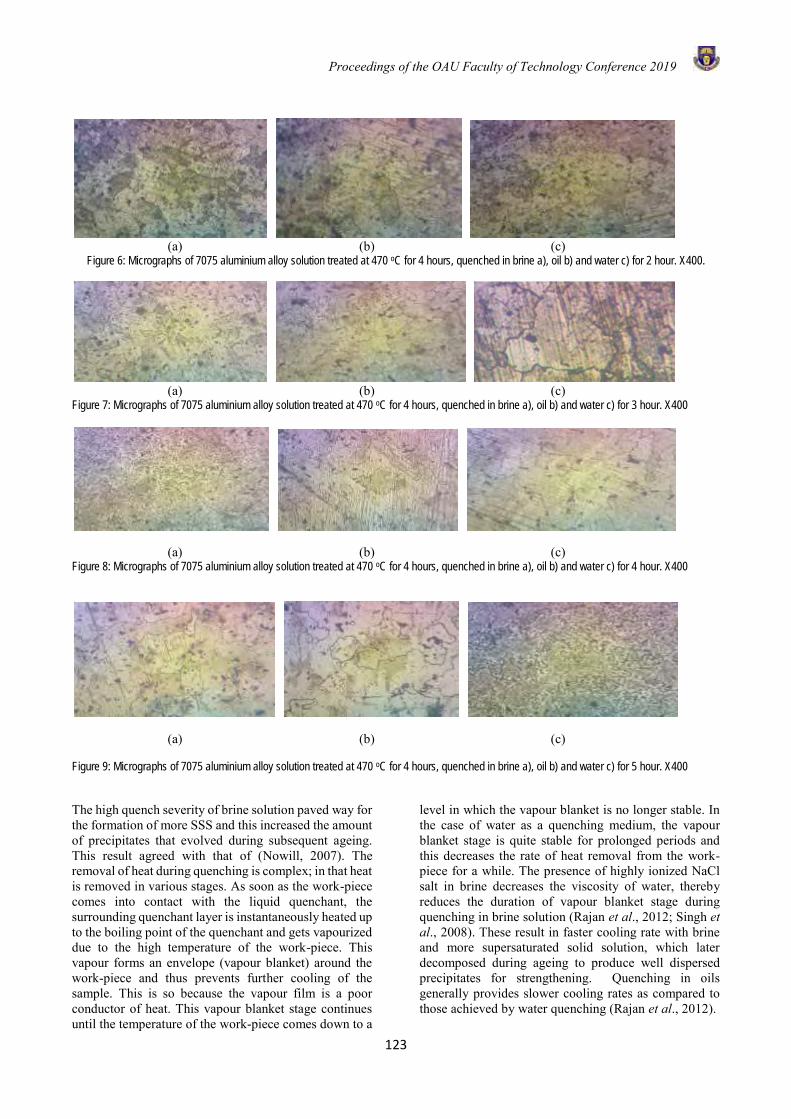
Proceedings of the OAU Faculty of Technology Conference 2019
123
(a) (b) (c)
Figure 6: Micrographs of 7075 aluminium alloy solution treated at 470 oC for 4 hours, quenched in brine a), oil b) and water c) for 2 hour. X400.
(a) (b) (c) Figure 7: Micrographs of 7075 aluminium alloy solution treated at 470 oC for 4 hours, quenched in brine a), oil b) and water c) for 3 hour. X400
(a) (b) (c) Figure 8: Micrographs of 7075 aluminium alloy solution treated at 470 oC for 4 hours, quenched in brine a), oil b) and water c) for 4 hour. X400
(a) (b) (c)
Figure 9: Micrographs of 7075 aluminium alloy solution treated at 470 oC for 4 hours, quenched in brine a), oil b) and water c) for 5 hour. X400
The high quench severity of brine solution paved way for the formation of more SSS and this increased the amount of precipitates that evolved during subsequent ageing. This result agreed with that of (Nowill, 2007). The removal of heat during quenching is complex; in that heat is removed in various stages. As soon as the work-piece comes into contact with the liquid quenchant, the surrounding quenchant layer is instantaneously heated up to the boiling point of the quenchant and gets vapourized due to the high temperature of the work-piece. This vapour forms an envelope (vapour blanket) around the work-piece and thus prevents further cooling of the sample. This is so because the vapour film is a poor conductor of heat. This vapour blanket stage continues until the temperature of the work-piece comes down to a
level in which the vapour blanket is no longer stable. In the case of water as a quenching medium, the vapour blanket stage is quite stable for prolonged periods and this decreases the rate of heat removal from the work-piece for a while. The presence of highly ionized NaCl salt in brine decreases the viscosity of water, thereby reduces the duration of vapour blanket stage during quenching in brine solution (Rajan et al., 2012; Singh et al., 2008). These result in faster cooling rate with brine and more supersaturated solid solution, which later decomposed during ageing to produce well dispersed precipitates for strengthening. Quenching in oils generally provides slower cooling rates as compared to those achieved by water quenching (Rajan et al., 2012).
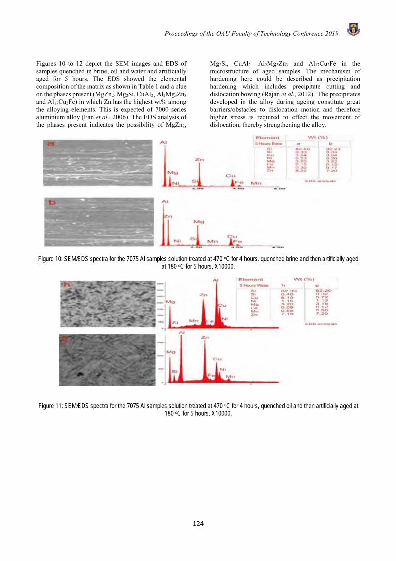
Proceedings of the OAU Faculty of Technology Conference 2019
124
Figures 10 to 12 depict the SEM images and EDS of samples quenched in brine, oil and water and artificially aged for 5 hours. The EDS showed the elemental composition of the matrix as shown in Table 1 and a clue on the phases present (MgZn2, Mg2Si, CuAl2¸ Al2Mg3Zn3 and Al17Cu2Fe) in which Zn has the highest wt% among the alloying elements. This is expected of 7000 series aluminium alloy (Fan et al., 2006). The EDS analysis of the phases present indicates the possibility of MgZn2,
Mg2Si, CuAl2¸ Al2Mg3Zn3 and Al17Cu2Fe in the microstructure of aged samples. The mechanism of hardening here could be described as precipitation hardening which includes precipitate cutting and dislocation bowing (Rajan et al., 2012). The precipitates developed in the alloy during ageing constitute great barriers/obstacles to dislocation motion and therefore higher stress is required to effect the movement of dislocation, thereby strengthening the alloy.
Figure 10: SEM/EDS spectra for the 7075 Al samples solution treated at 470 oC for 4 hours, quenched brine and then artificially aged at 180 oC for 5 hours, X10000.
Figure 11: SEM/EDS spectra for the 7075 Al samples solution treated at 470 oC for 4 hours, quenched oil and then artificially aged at 180 oC for 5 hours, X10000.
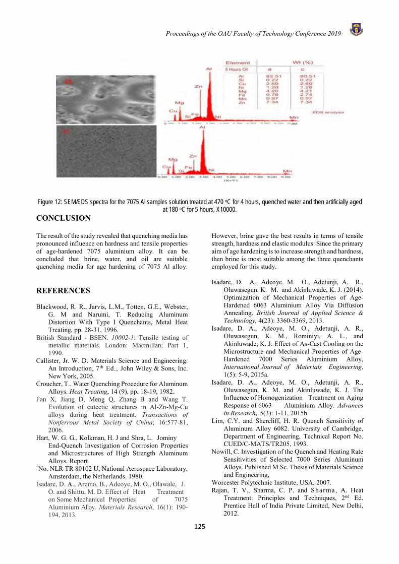
Proceedings of the OAU Faculty of Technology Conference 2019
125
Figure 12: SEM/EDS spectra for the 7075 Al samples solution treated at 470 oC for 4 hours, quenched water and then artificially aged at 180 oC for 5 hours, X10000.
CONCLUSION
The result of the study revealed that quenching media has pronounced influence on hardness and tensile properties of age-hardened 7075 aluminium alloy. It can be concluded that brine, water, and oil are suitable quenching media for age hardening of 7075 Al alloy.
However, brine gave the best results in terms of tensile strength, hardness and elastic modulus. Since the primary aim of age hardening is to increase strength and hardness, then brine is most suitable among the three quenchants employed for this study.
REFERENCES Blackwood, R. R., Jarvis, L.M., Totten, G.E., Webster,
G. M and Narumi, T. Reducing Aluminum Distortion With Type I Quenchants, Metal Heat Treating, pp. 28-31, 1996.
British Standard - BSEN. 10002-1: Tensile testing of metallic materials. London: Macmillan; Part 1, 1990.
Callister, Jr. W. D. Materials Science and Engineering: An Introduction, 7th Ed., John Wiley & Sons, Inc. New York, 2005.
Croucher, T.. Water Quenching Procedure for Aluminum Alloys. Heat Treating, 14 (9), pp. 18-19, 1982.
Fan X, Jiang D, Meng Q, Zhang B and Wang T. Evolution of eutectic structures in Al-Zn-Mg-Cu alloys during heat treatment. Transactions of Nonferrous Metal Society of China; 16:577-81, 2006.
Hart, W. G. G., Kolkman, H. J and Shra, L. Jominy End-Quench Investigation of Corrosion Properties and Microstructures of High Strength Aluminum Alloys. Report
`No. NLR TR 80102 U, National Aerospace Laboratory, Amsterdam, the Netherlands. 1980.
Isadare, D. A., Aremo, B., Adeoye, M. O., Olawale, J. O. and Shittu, M. D. Effect of Heat Treatment on Some Mechanical Properties of 7075 Aluminium Alloy. Materials Research, 16(1): 190-194, 2013.
Isadare, D. A., Adeoye, M. O., Adetunji, A. R., Oluwasegun, K. M. and Akinluwade, K. J. (2014). Optimization of Mechanical Properties of Age-Hardened 6063 Aluminium Alloy Via Diffusion Annealing. British Journal of Applied Science & Technology, 4(23): 3360-3369, 2013.
Isadare, D. A., Adeoye, M. O., Adetunji, A. R., Oluwasegun, K. M., Rominiyi, A. L., and Akinluwade, K. J. Effect of As-Cast Cooling on the Microstructure and Mechanical Properties of Age-Hardened 7000 Series Aluminium Alloy, International Journal of Materials Engineering, 1(5): 5-9, 2015a.
Isadare, D. A., Adeoye, M. O., Adetunji, A. R., Oluwasegun, K. M. and Akinluwade, K. J. The Influence of Homogenization Treatment on Aging Response of 6063 Aluminium Alloy. Advances in Research, 5(3): 1-11, 2015b.
Lim, C.Y. and Shercliff, H. R. Quench Sensitivity of Aluminum Alloy 6082. University of Cambridge, Department of Engineering, Technical Report No. CUED/C-MATS/TR205, 1993.
Nowill, C. Investigation of the Quench and Heating Rate Sensitivities of Selected 7000 Series Aluminum Alloys. Published M.Sc. Thesis of Materials Science and Engineering,
Worcester Polytechnic Institute, USA, 2007. Rajan, T. V., Sharma, C. P. and Sharma , A. Heat
Treatment: Principles and Techniques, 2nd Ed. Prentice Hall of India Private Limited, New Delhi, 2012.

Proceedings of the OAU Faculty of Technology Conference 2019
126
Singh, I. P., Chander, S. and Prasad, R. K. Materials Science and Engineering, 6th Ed. Jain Brothers, India, 2008.
Tensi, H. M., Stitzelberger-Jacob, P and Totten, G. E. Quenching Fundamentals: Surface Rewetting of
Aluminum. Adv. Mat. and Proc., 156(5), pp. H15-H20, 1999.
Totten, G. E and Webster, G. M. Quenching Fundamentals: Stability and Drag-Out of
Polymers. Adv. Mat. & Proc., 155(6), pp. H63-H66, 1999.
Proceedings of the OAU Faculty of Technology Conference 2019
127
A COMPARATIVE STUDY ON THE PHYSICAL PROPERTIES OF BRIQUETTES PRODUCED FROM CARBONIZED AND UNCARBONIZED
CORNCOB MATERIAL
T. F. Oyewusi1, E. F. Aransiola*2, T. E. Olaleye2, J. A. Osunbitan3 and L. A. O. Ogunjimi3 1Department of Agricultural Engineering, Adeleke University Ede, Osun State, Nigeria
2Department of Chemical Engineering, Obafemi Awolowo University, Ile-Ife, Osun-State, Nigeria 3Department of Agricultural and Environmental Engineering, Obafemi Awolowo University, Ile-Ife, Osun-State, Nigeria
*Email of Corresponding Author: [email protected]
ABSTRACT
In an effort to provide a more environment-friendly fuel alternative to the rural households in Nigeria, a study was carried out to compare some physical properties of briquettes from carbonized and uncarbonized corncob. Two forms of biomass processed materials (carbonized and uncarbonized corncobs) were compared and analysed through the determination of their physical properties in order to determine which of them are easier to handle and transport. For this study, three binders and three compaction pressure were used for the briquettes production. A charcoal kiln was fabricated for carbonized process of the corncob and a punch and die was also fabricated to facilitate the densification. The results of this study showed that average moisture content for the briquette produced from carbonized and uncarbonized corncob ranged between 5.29 – 6.58% (db), and 12.75 – 13.72 % (db), respectively. The mean relaxed density ranged between 813 – 925 kg/m3 and 963 – 1166 kg/m3 for the briquettes produced from carbonized and uncarbonized corncob, respectively. Also, the maximum and minimum compressive strength of briquettes produced were found to be 2.27 – 5.07 MPa and 5.97 – 10.12 MPa for carbonized and uncarbonized corncob, respectively. Thus, briquettes produced from uncarbonized corncob have more positive physical attributes of fuels in terms of density and compressive strength than briquettes produced from carbonized corncob. Keywords: Briquette; binder; compacting pressure; carbonized corncob; uncarbonized corncob INTRODUCTION In Nigeria, millions of tons of agricultural waste are generated annually, but it is quite unfortunate that farmers still practice “slash-and-burn” agriculture; in this instance most times, these agro-wastes produced during land clearing with other waste-by-products from agricultural processing activities are usually burnt off. According Fapetu (2000), valuable raw materials with potential energy are wasted by this exercise which further results in reduction in soil fertility and environmental pollution. Furthermore, most of these agro-wastes are not good enough to be used directly as fuel because they are colossal, uneven and have high moisture content and low densities, all these may cause problems in transportation and storage. However, they need to pass through some processes to reduce these problems. Degradation and environmental pollution are likely to occur if some of the agro-wastes are left to decay or burnt (Jekayinfa and Omisakin, 2005); hence, there is a need to convert these wastes into the form that alleviate the problem they pose when used directly. One of the promising solutions to these problems is the application of briquette technology. Wilaipon (2007) defined this technology as a densification process for improving the handling characteristics of raw materials and enhancing volumetric calorific value of the biomass. A briquette as defined by Grainger and Gibson (1981) is a block of compressed biomass or charcoal dust that is used as fuel to start and maintain fire. Two methods can
be employed in the production of briquettes, viz, carbonized and uncarbonized methods. Carbonized method is essentially the removal of volatile materials in the absence (or limited supply of) air; that is, the biomass is first partially burnt in an environment where air is totally controlled to give char product that is high in carbon. Uncarbonized is the method of making briquettes without first carbonizing, the raw material is prepared without allowing it to first pass through any form of heat or fire. Eriksson and Prior (1990) in their research found out that briquetting of biomass improves its handling characteristics, increase the volumetric calorific value, reduces transportation costs and makes it available for a variety of applications. Briquettes made from raw materials that cost nothing to obtain such as agricultural wastes can be an alternate source of domestic and industrial energy to charcoal, coal, electricity, firewood and gas. According to Fapetu (2000), the major source of energy to the rural community is fuel wood because other sources of energy (electricity, gas and kerosene) are either not available or grossly inadequate where available and beyond the reach of the masses. Hitherto, fuel wood collection has grave consequence on forest conservation and sustainable forest resource management. However, briquettes production reduces deforestation and its adverse effects thereby turns waste materials into fuel source. But depending on the materials used to make the briquettes, they may burn
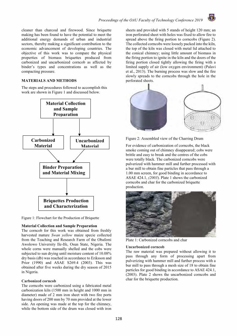
Proceedings of the OAU Faculty of Technology Conference 2019
128
cleaner than charcoal and firewood. Since briquette making has been found to have the potential to meet the additional energy demands of urban and industrial sectors, thereby making a significant contribution to the economic advancement of developing countries. The objective of this work was to compare the physical properties of biomass briquettes produced from carbonized and uncarbonized corncob as affected by binder’s types and concentrations as well as the compacting pressure. MATERIALS AND METHODS
The steps and procedures followed to accomplish this work are shown in Figure 1 and discussed below.
Figure 1: Flowchart for the Production of Briquette
Material Collection and Sample Preparation The corncob for this work was obtained from freshly harvested mature Swan yellow maize specie collected from the Teaching and Research Farm of the Obafemi Awolowo University Ile-Ife, Osun State, Nigeria. The whole corns were manually shelled and the cobs were subjected to sun drying until moisture content of 10.08% dry basis (db) was reached in accordance to Eriksson and Prior (1990) and ASAE S269.4 (2003). This was obtained after five weeks during the dry season of 2015 in Nigeria. Carbonized corncob The corncobs were carbonized using a fabricated metal carbonization kiln (1500 mm in height and 1000 mm in diameter) made of 2 mm iron sheet with two fire ports having doors of 200 mm by 70 mm provided at the lower side. An opening was made at the top for the chimney, while the bottom side of the drum was closed with iron
sheets and provided with 5 stands of height 120 mm; an iron perforated sheet with holes was fixed to allow fire to spread above the firing portion to corncobs (Figure 2). The collected corncobs were loosely packed into the kiln, the top of the kiln was closed with metal lid attached to the conical chimney; using little amount of biomass in the firing portion to ignite in the kiln and the doors of the firing portion closed tightly allowing the firing with a limited supply of air (low oxygen environment) (Palavi et al., 2013). The burning process was slow and the fire slowly spreads to the corncobs through the hole in the perforated sheets.
Figure 2: Assembled view of the Charring Drum
For evidence of carbonization of corncobs, the black smoke coming out of chimney disappeared; cobs were brittle and easy to break and the centres of the cobs were totally black. The carbonized corncobs were pulverized with hammer mill and further processed with a bur mill to obtain fine particles that pass through a 1.00 mm screen, for good binding in accordance to ASAE 424.1, (2003). Plate 1 shows the carbonized corncobs and char for the carbonized briquette production.
Plate 1: Carbonized corncobs and char
Uncarbonized corncob The raw material was prepared without allowing it to pass through any form of processing apart from pulverizing with hammer mill and further process with a bur mill to pass through a mesh size of 18 to obtain fine particles for good binding in accordance to ASAE 424.1, (2003). Plate 2 shows the uncarbonized corncobs and char for the briquette production.
Briquettes Production and Characterization
Material Collection and Sample Preparation
Carbonized Material
Uncarbonized Material
Binder Preparation and Material Mixing
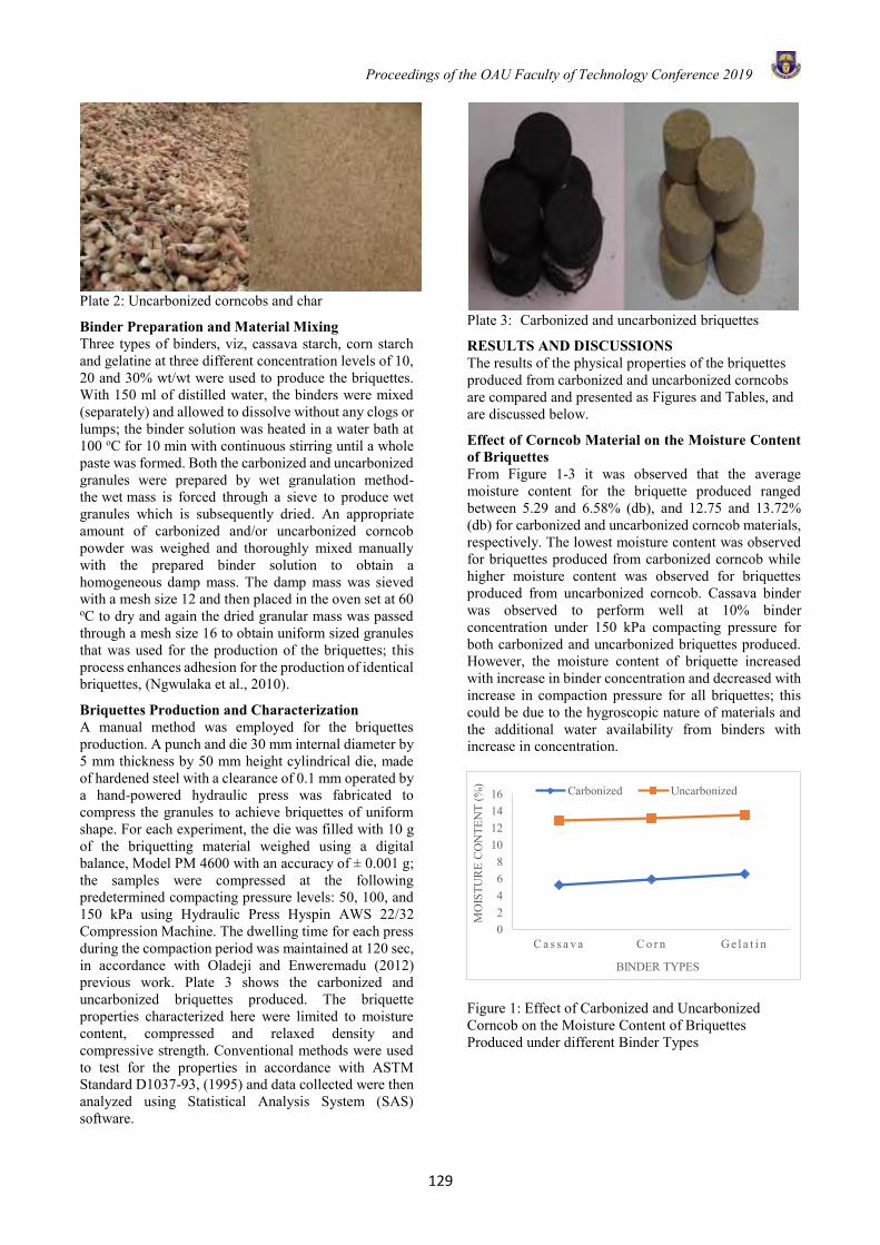
Proceedings of the OAU Faculty of Technology Conference 2019
129
Plate 2: Uncarbonized corncobs and char
Binder Preparation and Material Mixing Three types of binders, viz, cassava starch, corn starch and gelatine at three different concentration levels of 10, 20 and 30% wt/wt were used to produce the briquettes. With 150 ml of distilled water, the binders were mixed (separately) and allowed to dissolve without any clogs or lumps; the binder solution was heated in a water bath at 100 oC for 10 min with continuous stirring until a whole paste was formed. Both the carbonized and uncarbonized granules were prepared by wet granulation method- the wet mass is forced through a sieve to produce wet granules which is subsequently dried. An appropriate amount of carbonized and/or uncarbonized corncob powder was weighed and thoroughly mixed manually with the prepared binder solution to obtain a homogeneous damp mass. The damp mass was sieved with a mesh size 12 and then placed in the oven set at 60 oC to dry and again the dried granular mass was passed through a mesh size 16 to obtain uniform sized granules that was used for the production of the briquettes; this process enhances adhesion for the production of identical briquettes, (Ngwulaka et al., 2010).
Briquettes Production and Characterization A manual method was employed for the briquettes production. A punch and die 30 mm internal diameter by 5 mm thickness by 50 mm height cylindrical die, made of hardened steel with a clearance of 0.1 mm operated by a hand-powered hydraulic press was fabricated to compress the granules to achieve briquettes of uniform shape. For each experiment, the die was filled with 10 g of the briquetting material weighed using a digital balance, Model PM 4600 with an accuracy of ± 0.001 g; the samples were compressed at the following predetermined compacting pressure levels: 50, 100, and 150 kPa using Hydraulic Press Hyspin AWS 22/32 Compression Machine. The dwelling time for each press during the compaction period was maintained at 120 sec, in accordance with Oladeji and Enweremadu (2012) previous work. Plate 3 shows the carbonized and uncarbonized briquettes produced. The briquette properties characterized here were limited to moisture content, compressed and relaxed density and compressive strength. Conventional methods were used to test for the properties in accordance with ASTM Standard D1037-93, (1995) and data collected were then analyzed using Statistical Analysis System (SAS) software.
Plate 3: Carbonized and uncarbonized briquettes
RESULTS AND DISCUSSIONS The results of the physical properties of the briquettes produced from carbonized and uncarbonized corncobs are compared and presented as Figures and Tables, and are discussed below.
Effect of Corncob Material on the Moisture Content of Briquettes From Figure 1-3 it was observed that the average moisture content for the briquette produced ranged between 5.29 and 6.58% (db), and 12.75 and 13.72% (db) for carbonized and uncarbonized corncob materials, respectively. The lowest moisture content was observed for briquettes produced from carbonized corncob while higher moisture content was observed for briquettes produced from uncarbonized corncob. Cassava binder was observed to perform well at 10% binder concentration under 150 kPa compacting pressure for both carbonized and uncarbonized briquettes produced. However, the moisture content of briquette increased with increase in binder concentration and decreased with increase in compaction pressure for all briquettes; this could be due to the hygroscopic nature of materials and the additional water availability from binders with increase in concentration.
Figure 1: Effect of Carbonized and Uncarbonized Corncob on the Moisture Content of Briquettes Produced under different Binder Types
02468
10121416
C a s s a v a C o r n G e l a t i n
MO
ISTU
RE
CO
NTE
NT
(%)
BINDER TYPES
Carbonized Uncarbonized
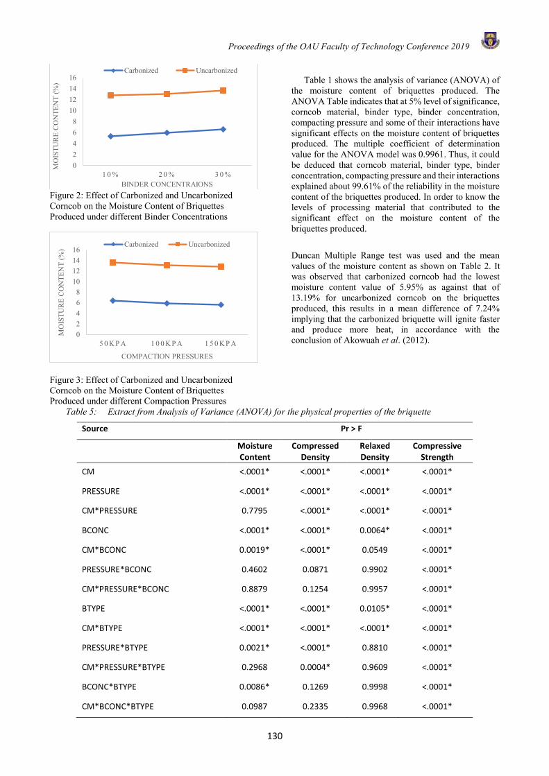
Proceedings of the OAU Faculty of Technology Conference 2019
130
Figure 2: Effect of Carbonized and Uncarbonized Corncob on the Moisture Content of Briquettes Produced under different Binder Concentrations
Figure 3: Effect of Carbonized and Uncarbonized Corncob on the Moisture Content of Briquettes Produced under different Compaction Pressures
Table 1 shows the analysis of variance (ANOVA) of
the moisture content of briquettes produced. The ANOVA Table indicates that at 5% level of significance, corncob material, binder type, binder concentration, compacting pressure and some of their interactions have significant effects on the moisture content of briquettes produced. The multiple coefficient of determination value for the ANOVA model was 0.9961. Thus, it could be deduced that corncob material, binder type, binder concentration, compacting pressure and their interactions explained about 99.61% of the reliability in the moisture content of the briquettes produced. In order to know the levels of processing material that contributed to the significant effect on the moisture content of the briquettes produced.
Duncan Multiple Range test was used and the mean values of the moisture content as shown on Table 2. It was observed that carbonized corncob had the lowest moisture content value of 5.95% as against that of 13.19% for uncarbonized corncob on the briquettes produced, this results in a mean difference of 7.24% implying that the carbonized briquette will ignite faster and produce more heat, in accordance with the conclusion of Akowuah et al. (2012).
Table 5: Extract from Analysis of Variance (ANOVA) for the physical properties of the briquette
Source Pr > F
Moisture Content
Compressed Density
Relaxed Density
Compressive Strength
CM <.0001* <.0001* <.0001* <.0001*
PRESSURE <.0001* <.0001* <.0001* <.0001*
CM*PRESSURE 0.7795 <.0001* <.0001* <.0001*
BCONC <.0001* <.0001* 0.0064* <.0001*
CM*BCONC 0.0019* <.0001* 0.0549 <.0001*
PRESSURE*BCONC 0.4602 0.0871 0.9902 <.0001*
CM*PRESSURE*BCONC 0.8879 0.1254 0.9957 <.0001*
BTYPE <.0001* <.0001* 0.0105* <.0001*
CM*BTYPE <.0001* <.0001* <.0001* <.0001*
PRESSURE*BTYPE 0.0021* <.0001* 0.8810 <.0001*
CM*PRESSURE*BTYPE 0.2968 0.0004* 0.9609 <.0001*
BCONC*BTYPE 0.0086* 0.1269 0.9998 <.0001*
CM*BCONC*BTYPE 0.0987 0.2335 0.9968 <.0001*
02468
10121416
1 0 % 2 0 % 3 0 %
MO
ISTU
RE
CO
NTE
NT
(%)
BINDER CONCENTRAIONS
Carbonized Uncarbonized
02468
10121416
5 0 K P A 1 0 0 K P A 1 5 0 K P A
MO
ISTU
RE
CO
NTE
NT
(%)
COMPACTION PRESSURES
Carbonized Uncarbonized
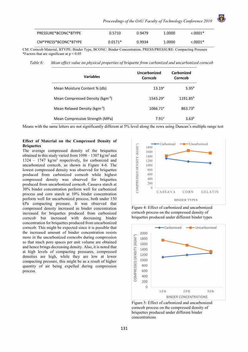
Proceedings of the OAU Faculty of Technology Conference 2019
131
PRESSURE*BCONC*BTYPE 0.5710 0.9479 1.0000 <.0001*
CM*PRESS*BCONC*BTYPE 0.0171* 0.9934 1.0000 <.0001*
CM: Corncob Material, BTYPE: Binder Type, BCONC: Binder Concentration, PRESS/PRESSURE: Compacting Pressure *Factors that are significant at p < 0.05
Table 6: Mean effect value on physical properties of briquette from carbonized and uncarbonized corncob
Variables Uncarbonized
Corncob Carbonized
Corncob
Mean Moisture Content % (db) 13.19a 5.95b
Mean Compressed Density (kgm-3) 1543.29a 1191.85b
Mean Relaxed Density (kgm-3) 1066.71a 863.73b
Mean Compressive Strength (MPa) 7.91a 3.63b
Means with the same letters are not significantly different at 5% level along the rows using Duncan’s multiple range test
Effect of Material on the Compressed Density of Briquettes The average compressed density of the briquettes obtained in this study varied from 1098 – 1307 kg/m3 and 1324 – 1747 kg/m3 respectively, for carbonized and uncarbonized corncob, as shown in Figure 4-6. The lowest compressed density was observed for briquettes produced from carbonized corncob while highest compressed density was observed for briquettes produced from uncarbonized corncob. Cassava starch at 30% binder concentration perform well for carbonized process and corn starch at 10% binder concentration perform well for uncarbonized process, both under 150 kPa compacting pressure. It was observed that compressed density increased as binder concentration increased for briquettes produced from carbonized corncob but increased with decreasing binder concentration for briquettes produced from uncarbonized corncob. This might be expected since it is possible that the increased amount of binder concentration resists more in the uncarbonized corncobs during compression so that much pore spaces per unit volume are obtained and hence brings decreasing density. Also, it is noted that at high levels of compacting pressures, compressed densities are high, while they are low at lower compacting pressure, this might be as a result of higher quantity of air being expelled during compression process.
Figure 4: Effect of carbonized and uncarbonized corncob process on the compressed density of briquettes produced under different binder types
Figure 5: Effect of carbonized and uncarbonized corncob process on the compressed density of briquettes produced under different binder concentrations
0200400600800
10001200140016001800
C A S S A V A C O R N G E LA T I NCO
MPR
ESSE
D D
ENSI
TY (K
GM
-3)
BINDER TYPES
Carbonized Uncarbonized
0
200
400
600
800
1000
1200
1400
1600
1800
2000
1 0 % 2 0 % 3 0 %
CO
MP
RES
SED
DEN
SITY
(K
GM
-3)
BINDER CONCENTRATIONS
Carbonized Uncarbonized
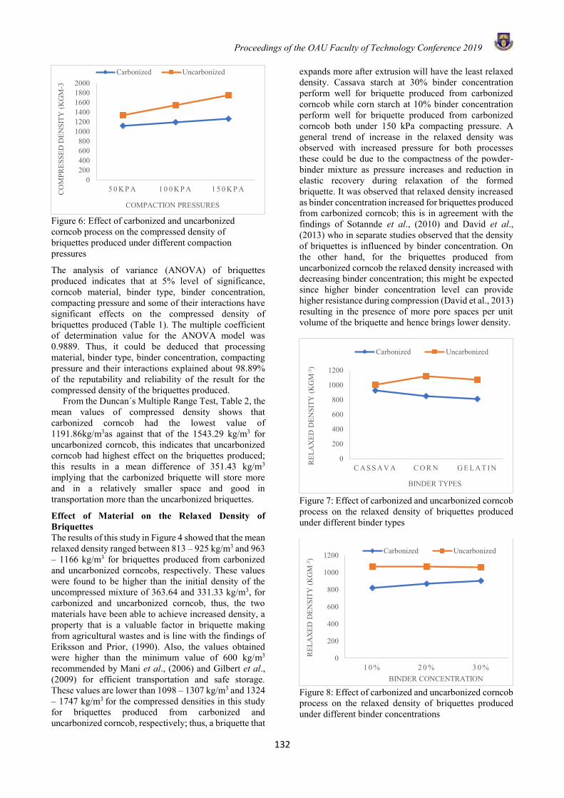
Proceedings of the OAU Faculty of Technology Conference 2019
132
Figure 6: Effect of carbonized and uncarbonized corncob process on the compressed density of briquettes produced under different compaction pressures
The analysis of variance (ANOVA) of briquettes produced indicates that at 5% level of significance, corncob material, binder type, binder concentration, compacting pressure and some of their interactions have significant effects on the compressed density of briquettes produced (Table 1). The multiple coefficient of determination value for the ANOVA model was 0.9889. Thus, it could be deduced that processing material, binder type, binder concentration, compacting pressure and their interactions explained about 98.89% of the reputability and reliability of the result for the compressed density of the briquettes produced.
From the Duncan´s Multiple Range Test, Table 2, the mean values of compressed density shows that carbonized corncob had the lowest value of 1191.86kg/m3as against that of the 1543.29 kg/m3 for uncarbonized corncob, this indicates that uncarbonized corncob had highest effect on the briquettes produced; this results in a mean difference of 351.43 kg/m3 implying that the carbonized briquette will store more and in a relatively smaller space and good in transportation more than the uncarbonized briquettes.
Effect of Material on the Relaxed Density of Briquettes The results of this study in Figure 4 showed that the mean relaxed density ranged between 813 – 925 kg/m3 and 963 – 1166 kg/m3 for briquettes produced from carbonized and uncarbonized corncobs, respectively. These values were found to be higher than the initial density of the uncompressed mixture of 363.64 and 331.33 kg/m3, for carbonized and uncarbonized corncob, thus, the two materials have been able to achieve increased density, a property that is a valuable factor in briquette making from agricultural wastes and is line with the findings of Eriksson and Prior, (1990). Also, the values obtained were higher than the minimum value of 600 kg/m3
recommended by Mani et al., (2006) and Gilbert et al., (2009) for efficient transportation and safe storage. These values are lower than 1098 – 1307 kg/m3 and 1324 – 1747 kg/m3 for the compressed densities in this study for briquettes produced from carbonized and uncarbonized corncob, respectively; thus, a briquette that
expands more after extrusion will have the least relaxed density. Cassava starch at 30% binder concentration perform well for briquette produced from carbonized corncob while corn starch at 10% binder concentration perform well for briquette produced from carbonized corncob both under 150 kPa compacting pressure. A general trend of increase in the relaxed density was observed with increased pressure for both processes these could be due to the compactness of the powder-binder mixture as pressure increases and reduction in elastic recovery during relaxation of the formed briquette. It was observed that relaxed density increased as binder concentration increased for briquettes produced from carbonized corncob; this is in agreement with the findings of Sotannde et al., (2010) and David et al., (2013) who in separate studies observed that the density of briquettes is influenced by binder concentration. On the other hand, for the briquettes produced from uncarbonized corncob the relaxed density increased with decreasing binder concentration; this might be expected since higher binder concentration level can provide higher resistance during compression (David et al., 2013) resulting in the presence of more pore spaces per unit volume of the briquette and hence brings lower density.
Figure 7: Effect of carbonized and uncarbonized corncob process on the relaxed density of briquettes produced under different binder types
Figure 8: Effect of carbonized and uncarbonized corncob process on the relaxed density of briquettes produced under different binder concentrations
0200400600800
100012001400160018002000
5 0 K P A 1 0 0 K P A 1 5 0 K P ACO
MPR
ESSE
D D
ENSI
TY (K
GM
-3
COMPACTION PRESSURES
Carbonized Uncarbonized
0
200
400
600
800
1000
1200
C A S S A V A C O R N G E LA T I N
REL
AX
ED D
ENSI
TY (K
GM
-3)
BINDER TYPES
Carbonized Uncarbonized
0
200
400
600
800
1000
1200
1 0 % 2 0 % 3 0 %
REL
AX
ED D
ENSI
TY (K
GM
-3)
BINDER CONCENTRATION
Carbonized Uncarbonized
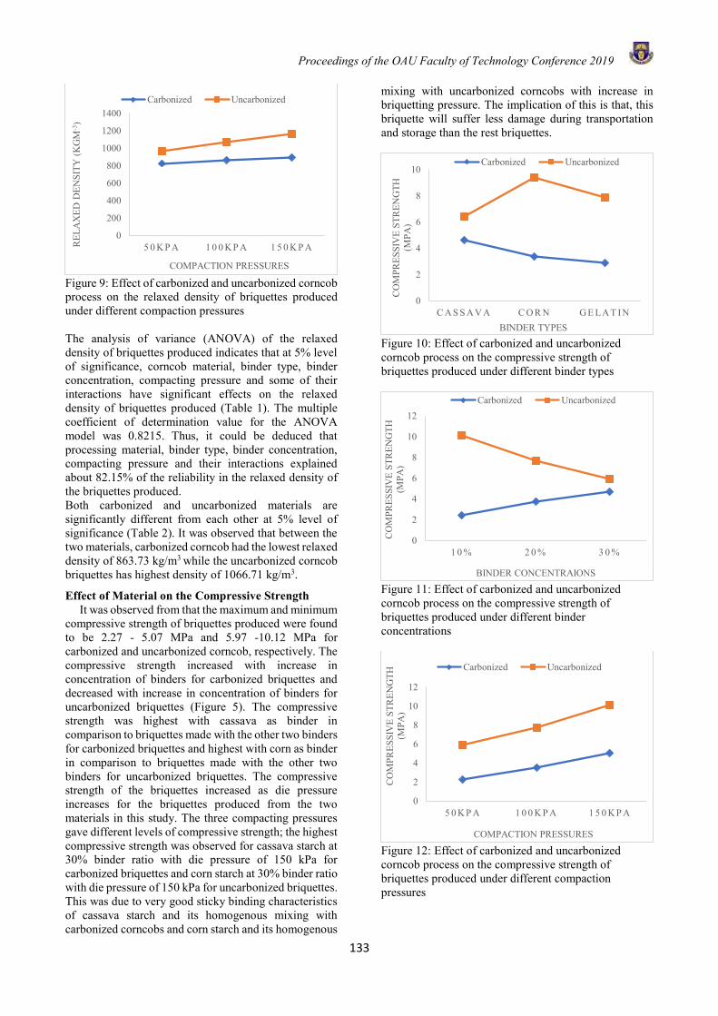
Proceedings of the OAU Faculty of Technology Conference 2019
133
Figure 9: Effect of carbonized and uncarbonized corncob process on the relaxed density of briquettes produced under different compaction pressures The analysis of variance (ANOVA) of the relaxed density of briquettes produced indicates that at 5% level of significance, corncob material, binder type, binder concentration, compacting pressure and some of their interactions have significant effects on the relaxed density of briquettes produced (Table 1). The multiple coefficient of determination value for the ANOVA model was 0.8215. Thus, it could be deduced that processing material, binder type, binder concentration, compacting pressure and their interactions explained about 82.15% of the reliability in the relaxed density of the briquettes produced. Both carbonized and uncarbonized materials are significantly different from each other at 5% level of significance (Table 2). It was observed that between the two materials, carbonized corncob had the lowest relaxed density of 863.73 kg/m3 while the uncarbonized corncob briquettes has highest density of 1066.71 kg/m3.
Effect of Material on the Compressive Strength It was observed from that the maximum and minimum
compressive strength of briquettes produced were found to be 2.27 - 5.07 MPa and 5.97 -10.12 MPa for carbonized and uncarbonized corncob, respectively. The compressive strength increased with increase in concentration of binders for carbonized briquettes and decreased with increase in concentration of binders for uncarbonized briquettes (Figure 5). The compressive strength was highest with cassava as binder in comparison to briquettes made with the other two binders for carbonized briquettes and highest with corn as binder in comparison to briquettes made with the other two binders for uncarbonized briquettes. The compressive strength of the briquettes increased as die pressure increases for the briquettes produced from the two materials in this study. The three compacting pressures gave different levels of compressive strength; the highest compressive strength was observed for cassava starch at 30% binder ratio with die pressure of 150 kPa for carbonized briquettes and corn starch at 30% binder ratio with die pressure of 150 kPa for uncarbonized briquettes. This was due to very good sticky binding characteristics of cassava starch and its homogenous mixing with carbonized corncobs and corn starch and its homogenous
mixing with uncarbonized corncobs with increase in briquetting pressure. The implication of this is that, this briquette will suffer less damage during transportation and storage than the rest briquettes.
Figure 10: Effect of carbonized and uncarbonized corncob process on the compressive strength of briquettes produced under different binder types
Figure 11: Effect of carbonized and uncarbonized corncob process on the compressive strength of briquettes produced under different binder concentrations
Figure 12: Effect of carbonized and uncarbonized corncob process on the compressive strength of briquettes produced under different compaction pressures
0
200
400
600
800
1000
1200
1400
5 0 K P A 1 0 0 K P A 1 5 0 K P AREL
AX
ED D
ENSI
TY (K
GM
-3)
COMPACTION PRESSURES
Carbonized Uncarbonized
0
2
4
6
8
10
C A S S A V A C O R N G E LA T I N
CO
MPR
ESSI
VE
STR
ENG
TH
(MPA
)
BINDER TYPES
Carbonized Uncarbonized
0
2
4
6
8
10
12
1 0 % 2 0 % 3 0 %
CO
MPR
ESSI
VE
STR
ENG
TH
(MPA
)
BINDER CONCENTRAIONS
Carbonized Uncarbonized
0
2
4
6
8
10
12
5 0 K P A 1 0 0 K P A 1 5 0 K P A
CO
MPR
ESSI
VE
STR
ENG
TH
(MPA
)
COMPACTION PRESSURES
Carbonized Uncarbonized
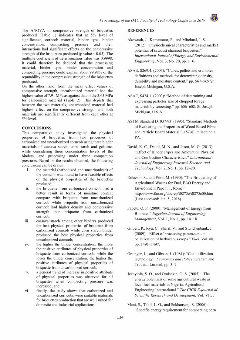
Proceedings of the OAU Faculty of Technology Conference 2019
134
The ANOVA of compressive strength of briquettes produced (Table 1) indicates that at 5% level of significance, corncob material, binder type, binder concentration, compacting pressure and their interactions had significant effects on the compressive strength of the briquettes produced (p value < 0.05). The multiple coefficient of determination value was 0.9998. It could therefore be deduced that the processing material, binder type, binder concentration and compacting pressure could explain about 99.98% of the reputability in the compressive strength of the briquettes produced. On the other hand, from the mean effect values of compressive strength, uncarbonized material had the highest value of 7.91 MPa as against that of the 3.63 MPa for carbonized material (Table 2). This depicts that between the two materials, uncarbonized material had highest effect on the compressive strength and both materials are significantly different from each other at 5% level. CONCLUSIONS This comparative study investigated the physical properties of briquettes from two processes of carbonized and uncarbonized corncob using three binder materials of cassava starch, corn starch and gelatine; while considering three concentration levels of the binders, and processing under three compaction pressures. Based on the results obtained, the following conclusions can be drawn:
i. the material (carbonized and uncarbonized) of the corncob was found to have feasible effects on the physical properties of the briquettes produced;
ii. the briquette from carbonized corncob had a better result in terms of moisture content compare with briquette from uncarbonized corncob while briquette from uncarbonized corncob had higher density and compressive strength than briquette from carbonized corncob;
iii. cassava starch among other binders produced the best physical properties of briquette from carbonized corncob while corn starch binder produced the best physical properties from uncarbonized corncob;
iv. the higher the binder concentration, the more the positive attributes of physical properties of briquette from carbonized corncob; while the lower the binder concentration, the higher the positive attributes of physical properties of briquette from uncarbonized corncob;
v. a general trend of increase in positive attribute of physical properties was observed for all briquettes when compacting pressure was increased; and
vi. finally, the study shows that carbonized and uncarbonized corncobs were suitable materials for briquettes production that are well suited for domestic and industrial applications.
REFERENCES Akowuah, J., Kemausuor, F., and Mitchual, J. S.
(2012): “Physiochemical characteristics and market potential of sawdust charcoal briquettes.” International Journal of Energy and Environmental Engineering, Vol. 3, No. 20, pp. 1−6.
ASAE, S269.4. (2003): “Cubes, pellets and crumbles – definitions and methods for determining density, durability and moisture content.” pp. 567–569 St. Joseph Michigan, U.S.A.
ASAE, S424.1. (2003): “Method of determining and expressing particles size of chopped forage materials by screening.” pp. 606–608. St. Joseph Michigan, U.S.A.
ASTM Standard D1037-93. (1995): “Standard Methods of Evaluating the Properties of Wood Based Fibre and Particle Board Material.” ASTM, Philadelphia, PA.
David, K. C., Daudi, M. N., and Jason, M. G. (2013): “Effect of Binder Types and Amount on Physical and Combustion Characteristics.” International Journal of Engineering Research Science, and Technology, Vol. 2, No. 1, pp. 12–20.
Eriksson, S., and Prior, M. (1990): “The Briquetting of Agricultural Wastes for Fuel, FAO Energy and Environment Paper 11, Rome.” http://www.fao.org/docrep/t0275e/t0275e00.htm (Last accessed: Jan. 5, 2018).
Fapetu, O. P. (2000): “Management of Energy from Biomass.” Nigerian Journal of Engineering Management, Vol. 1, No. 1, pp. 14–18.
Gilbert, P., Ryu, C., Sharif, V., and Switchenbank, J. (2009): “Effect of processing parameters on pelletization of herbaceous crops.” Fuel, Vol. 88, pp. 1491–1497.
Grainger, L., and Gibson, J. (1981): “Coal utilization technology.” Economics and Policy, Graham and Trotman Limited, pp. 3–7.
Jekayinfa, S. O., and Omisakin, O. S. (2005): “The energy potentials of some agricultural waste as local fuel materials in Nigeria, Agricultural Engineering International.” The CIGR E-journal of Scientific Research and Development, Vol. VII, .
Mani, S., Tabil, L. G., and Sokhansanj, S. (2006): “Specific energy requirement for compacting corn

Proceedings of the OAU Faculty of Technology Conference 2019
135
stover.” Bioresource Technology, Vol. 97, pp. 1420–1426.
Ngwulaka, N. C., Idiakhoa, B. A., Nep, E. I., Ogaji, I., and Okafor, I. S. (2010): “Formulation and evaluation of paracetamol tablets manufactured using the dried fruit of Phoenix dactylifera Linn as an excipient.” Research in Pharmaceutical Biotechnology, Vol. 2, No. 3, pp. 25–32.
Oladeji, J. T., and Enweremadu, C. C. (2012): “The Effects of Some Processing Parameters on Physical and Combustion Characteristics of Corncob Briquettes.” International Journal of Energy Engineering, Vol. 2, No. 1, pp. 22–27.
Palavi, H. V., Srikantaswamy, S., Kiran, B. M., Vyshnavi, D. R., and Ashwin, C. A. (2013): “Briquetting Agricultural Waste as an Energy Source.” Journal of Environmental Science, Computer Science and Engineering and Technology, Vol. 2, No. 1, pp. 160–172.
Sotannde, O., Oluyege, G., and Abah, B. (2010): “Physical and Combustion Properties of Briquettes from Sawdust of Azadirachtaindica.” Journal of Forestry Research, Vol. 21, pp. 63–67.
Wilaipon, P. (2007): “Physical Characteristics of Maize Cob Briquettes under Moderate Die Pressure.” American Journal of Applied Science, Vol. 4, pp. 995–998.
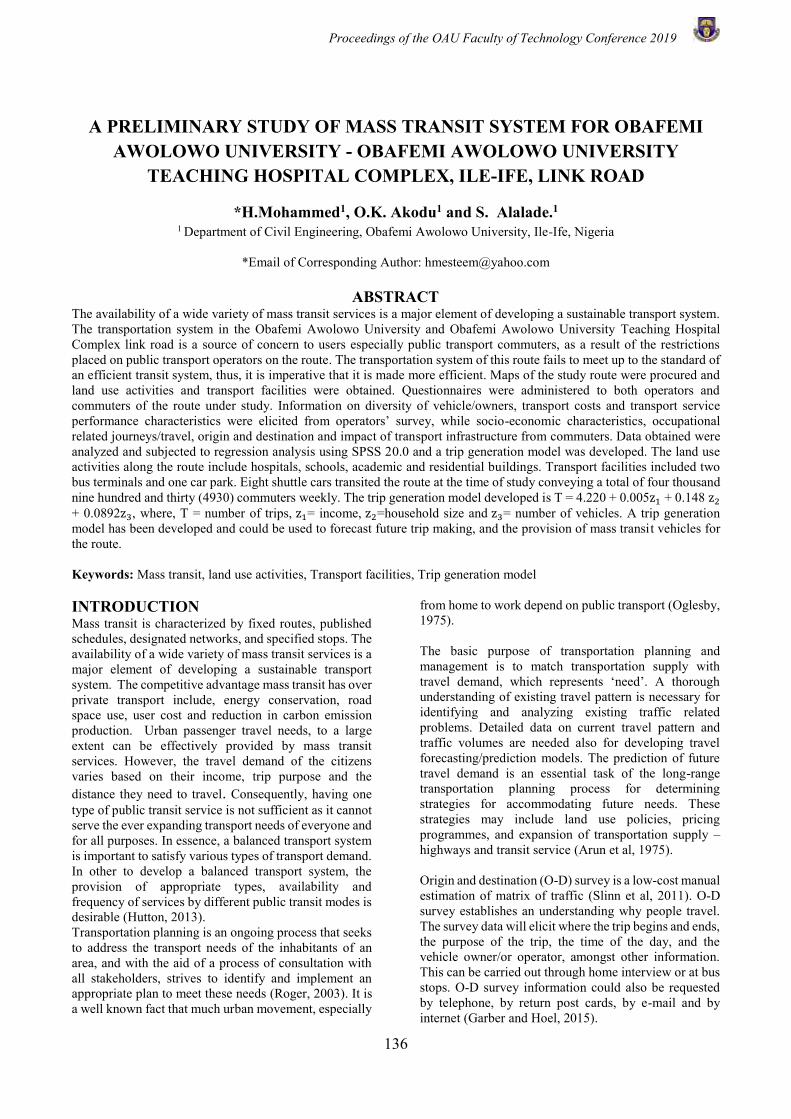
Proceedings of the OAU Faculty of Technology Conference 2019
136
A PRELIMINARY STUDY OF MASS TRANSIT SYSTEM FOR OBAFEMI AWOLOWO UNIVERSITY - OBAFEMI AWOLOWO UNIVERSITY
TEACHING HOSPITAL COMPLEX, ILE-IFE, LINK ROAD
*H.Mohammed1, O.K. Akodu1 and S. Alalade.1 1 Department of Civil Engineering, Obafemi Awolowo University, Ile-Ife, Nigeria
*Email of Corresponding Author: [email protected]
ABSTRACT The availability of a wide variety of mass transit services is a major element of developing a sustainable transport system. The transportation system in the Obafemi Awolowo University and Obafemi Awolowo University Teaching Hospital Complex link road is a source of concern to users especially public transport commuters, as a result of the restrictions placed on public transport operators on the route. The transportation system of this route fails to meet up to the standard of an efficient transit system, thus, it is imperative that it is made more efficient. Maps of the study route were procured and land use activities and transport facilities were obtained. Questionnaires were administered to both operators and commuters of the route under study. Information on diversity of vehicle/owners, transport costs and transport service performance characteristics were elicited from operators’ survey, while socio-economic characteristics, occupational related journeys/travel, origin and destination and impact of transport infrastructure from commuters. Data obtained were analyzed and subjected to regression analysis using SPSS 20.0 and a trip generation model was developed. The land use activities along the route include hospitals, schools, academic and residential buildings. Transport facilities included two bus terminals and one car park. Eight shuttle cars transited the route at the time of study conveying a total of four thousand nine hundred and thirty (4930) commuters weekly. The trip generation model developed is T = 4.220 + 0.005z1 + 0.148 z2 + 0.0892z3, where, T = number of trips, z1= income, z2=household size and z3= number of vehicles. A trip generation model has been developed and could be used to forecast future trip making, and the provision of mass transit vehicles for the route. Keywords: Mass transit, land use activities, Transport facilities, Trip generation model INTRODUCTION Mass transit is characterized by fixed routes, published schedules, designated networks, and specified stops. The availability of a wide variety of mass transit services is a major element of developing a sustainable transport system. The competitive advantage mass transit has over private transport include, energy conservation, road space use, user cost and reduction in carbon emission production. Urban passenger travel needs, to a large extent can be effectively provided by mass transit services. However, the travel demand of the citizens varies based on their income, trip purpose and the distance they need to travel. Consequently, having one type of public transit service is not sufficient as it cannot serve the ever expanding transport needs of everyone and for all purposes. In essence, a balanced transport system is important to satisfy various types of transport demand. In other to develop a balanced transport system, the provision of appropriate types, availability and frequency of services by different public transit modes is desirable (Hutton, 2013). Transportation planning is an ongoing process that seeks to address the transport needs of the inhabitants of an area, and with the aid of a process of consultation with all stakeholders, strives to identify and implement an appropriate plan to meet these needs (Roger, 2003). It is a well known fact that much urban movement, especially
from home to work depend on public transport (Oglesby, 1975). The basic purpose of transportation planning and management is to match transportation supply with travel demand, which represents ‘need’. A thorough understanding of existing travel pattern is necessary for identifying and analyzing existing traffic related problems. Detailed data on current travel pattern and traffic volumes are needed also for developing travel forecasting/prediction models. The prediction of future travel demand is an essential task of the long-range transportation planning process for determining strategies for accommodating future needs. These strategies may include land use policies, pricing programmes, and expansion of transportation supply – highways and transit service (Arun et al, 1975). Origin and destination (O-D) survey is a low-cost manual estimation of matrix of traffic (Slinn et al, 2011). O-D survey establishes an understanding why people travel. The survey data will elicit where the trip begins and ends, the purpose of the trip, the time of the day, and the vehicle owner/or operator, amongst other information. This can be carried out through home interview or at bus stops. O-D survey information could also be requested by telephone, by return post cards, by e-mail and by internet (Garber and Hoel, 2015).
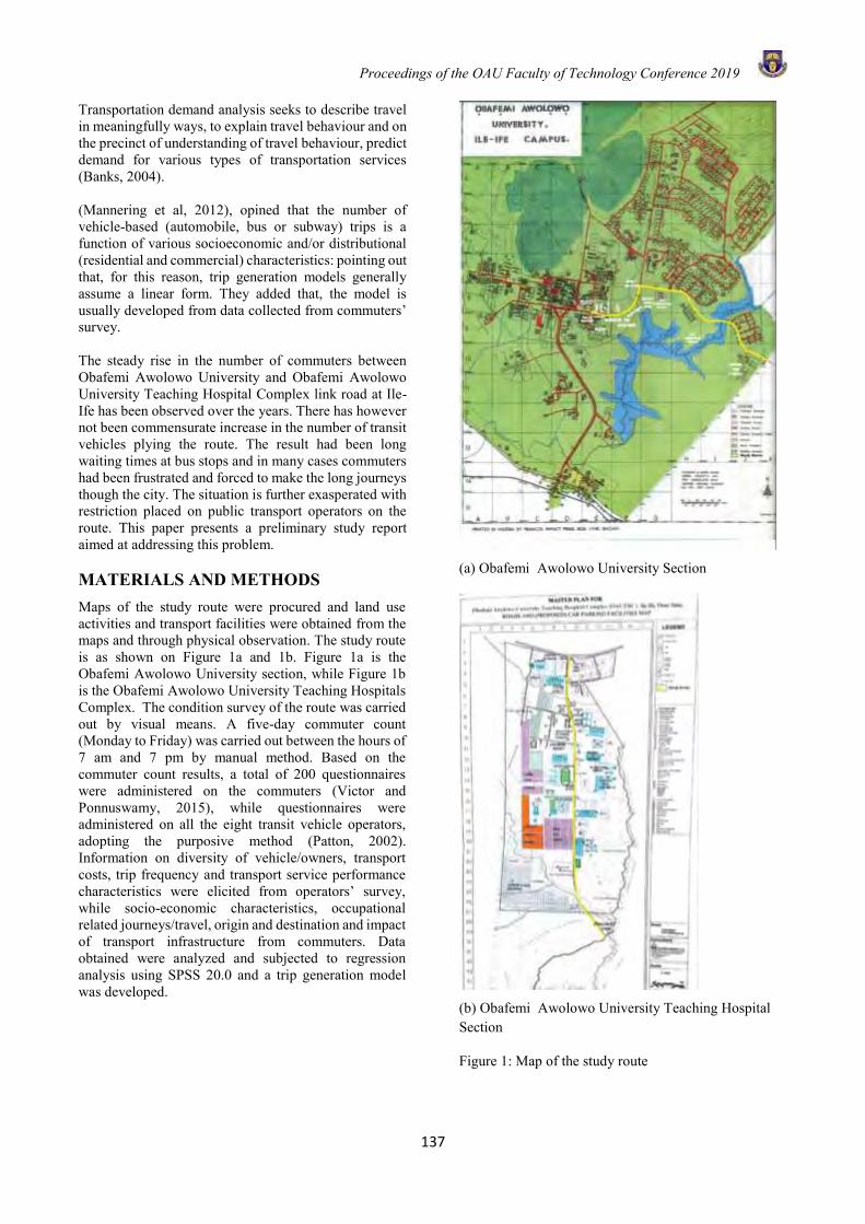
Proceedings of the OAU Faculty of Technology Conference 2019
137
Transportation demand analysis seeks to describe travel in meaningfully ways, to explain travel behaviour and on the precinct of understanding of travel behaviour, predict demand for various types of transportation services (Banks, 2004). (Mannering et al, 2012), opined that the number of vehicle-based (automobile, bus or subway) trips is a function of various socioeconomic and/or distributional (residential and commercial) characteristics: pointing out that, for this reason, trip generation models generally assume a linear form. They added that, the model is usually developed from data collected from commuters’ survey. The steady rise in the number of commuters between Obafemi Awolowo University and Obafemi Awolowo University Teaching Hospital Complex link road at Ile-Ife has been observed over the years. There has however not been commensurate increase in the number of transit vehicles plying the route. The result had been long waiting times at bus stops and in many cases commuters had been frustrated and forced to make the long journeys though the city. The situation is further exasperated with restriction placed on public transport operators on the route. This paper presents a preliminary study report aimed at addressing this problem. MATERIALS AND METHODS Maps of the study route were procured and land use activities and transport facilities were obtained from the maps and through physical observation. The study route is as shown on Figure 1a and 1b. Figure 1a is the Obafemi Awolowo University section, while Figure 1b is the Obafemi Awolowo University Teaching Hospitals Complex. The condition survey of the route was carried out by visual means. A five-day commuter count (Monday to Friday) was carried out between the hours of 7 am and 7 pm by manual method. Based on the commuter count results, a total of 200 questionnaires were administered on the commuters (Victor and Ponnuswamy, 2015), while questionnaires were administered on all the eight transit vehicle operators, adopting the purposive method (Patton, 2002). Information on diversity of vehicle/owners, transport costs, trip frequency and transport service performance characteristics were elicited from operators’ survey, while socio-economic characteristics, occupational related journeys/travel, origin and destination and impact of transport infrastructure from commuters. Data obtained were analyzed and subjected to regression analysis using SPSS 20.0 and a trip generation model was developed.
(a) Obafemi Awolowo University Section
(b) Obafemi Awolowo University Teaching Hospital Section
Figure 1: Map of the study route

Proceedings of the OAU Faculty of Technology Conference 2019
138
RESULTS AND DISCUSSION The road section is a single lane carriageway of asphaltic concrete finish with a total length of 6.8km. The land use activities along the route include hospitals, schools, academic and residential buildings. Transport facilities included two terminals and one car park. There are no designated bus stops. This denotes a lack of this facility on the route. Table 1shows that, there are intermediate stops. Condition survey of the route showed that the route is generally in good condition, but there are isolated points of failure typified by pot holes, crocodile cracks, longitudinal and traverse cracks, and rutting. Figure 2 shows the distribution of commuters on the route. It is observed that the highest number of commuters use the route on Tuesday. This is typical of workers and students, as returns from weekends peaks on Tuesdays. The lowest figure recorded for Friday, is instructive of approach of weekend. The hourly distribution of the commuters is as shown on Figure 3. The distribution is normal for work and school journeys as depicted by early morning rush (7am – 8am), and return hour peaks between 1pm and 3pm.The average volume of commuters is 986/day. This is veritable information for bus schedules. This volume of commuters obtained, informed the decision to adopt a sample size for the distribution of commuter survey questionnaires of 200 (Salter and Hounsell, 1996). The age distribution of the commuters is as shown in Figure 4 while the occupation distribution is as shown on Figure 5. These results corroborate one another as the
age bracket of 21-30 years (Tertiary students’ age) in Figure 4 which has the highest figure of 57 % and Figure 5, which indicates the highest figure of 51% for students. This portends that commuter trips are mainly academic related ones.Eight, five-passenger- seated Nissan Micra vehicles transit the route daily and all are operator driven. A fee of N50 is charged per drop at any point along the route and there is no variation in this charge at any time of the year. 16.7% of the operators make the trips from OAUTHC end about 18 times daily, 66.67%, 20 times daily and 16.7% 30 times. Figure 6 shows the monthly income distribution of the commuters. 45.5 % earn between ₦ 5000 and ₦ 15,000, and 21 % earn between ₦ 16,000 and ₦25,000, monthly. The distribution is a true reflection of the predominance of students as the major commuters on the route. The trip making frequency of the commuters on the route is as shown on Figure 7. 58 % of the commuters make the trips five times a week. This shows that most of the trips are academic/work related journeys, a major feature of the land use activity along the route. Figure 8 shows private vehicle accessibility by the commuters. 30 % have no access to vehicle while 32 % have access to one vehicle. This combine pool of commuters (60 %) is an indication of the viability of the route for the provision of mass transit vehicle. Figure 9 shows the waiting period of commuters at traffic generating points. 72 % spend between 21 and 30 minutes waiting to board the available transit vehicles. This is a further indication of the need for mass transit system for the route.
Table 1: Origin and Destination Survey Data Showing the Number of Commuters at Traffic Generating Points
Origin OAUTHC OAU Total Percentage (%) OAU Campus 90 - 90 45%
OAU Teaching Hospital
- 87 87 43.5%
Junior Staff quarters
2 3 5 2.5%
OAU International School
2 7 9 4.5%
OAU Staff School 1 0 1 0.5% Moremi High School
1 3 4 2%
OAU Primary School
1 0 1 0.5%
Road 7 Junction 1 0 1 0.5% Phase 2 2 0 2 1%
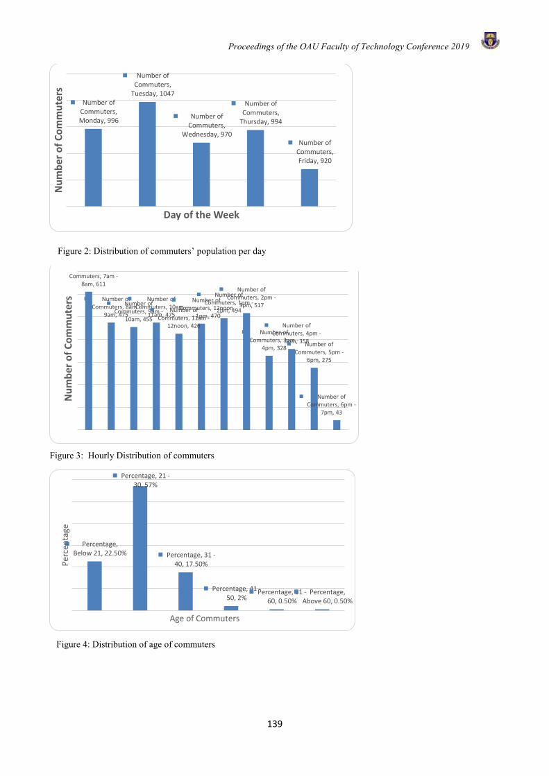
Proceedings of the OAU Faculty of Technology Conference 2019
139
Figure 3: Hourly Distribution of commuters
Number of Commuters, Monday, 996
Number of Commuters,
Tuesday, 1047
Number of Commuters,
Wednesday, 970
Number of Commuters,
Thursday, 994
Number of Commuters, Friday, 920
Nu
mb
er o
f C
om
mu
ters
Day of the Week
Number of Commuters, 7am -
8am, 611
Number of Commuters, 8am -
9am, 475
Number of Commuters, 9am -
10am, 455
Number of Commuters, 10am -
11am, 475Number of
Commuters, 11am -12noon, 426
Number of Commuters, 12noon
- 1pm, 470
Number of Commuters, 1pm -
2pm, 494
Number of Commuters, 2pm -
3pm, 517
Number of Commuters, 3pm -
4pm, 328
Number of Commuters, 4pm -
5pm, 358Number of Commuters, 5pm -
6pm, 275
Number of Commuters, 6pm -
7pm, 43
Nu
mb
er o
f C
om
mu
ters
Percentage, Below 21, 22.50%
Percentage, 21 -30, 57%
Percentage, 31 -40, 17.50%
Percentage, 41 -50, 2%
Percentage, 51 -60, 0.50%
Percentage, Above 60, 0.50%
Per
cen
tage
Age of Commuters
Figure 2: Distribution of commuters’ population per day
Figure 4: Distribution of age of commuters
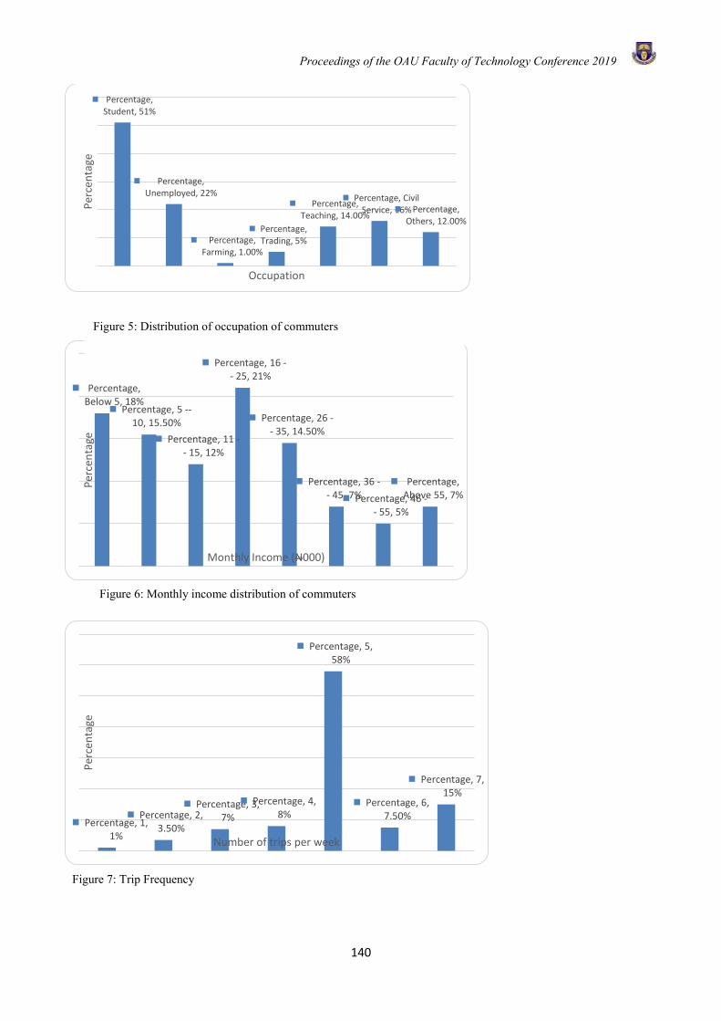
Proceedings of the OAU Faculty of Technology Conference 2019
140
Percentage, Student, 51%
Percentage, Unemployed, 22%
Percentage, Farming, 1.00%
Percentage, Trading, 5%
Percentage, Teaching, 14.00%
Percentage, Civil Service, 16% Percentage,
Others, 12.00%
Per
cen
tage
Occupation
Percentage, Below 5, 18%
Percentage, 5 --10, 15.50%
Percentage, 11 -- 15, 12%
Percentage, 16 -- 25, 21%
Percentage, 26 -- 35, 14.50%
Percentage, 36 -- 45, 7%Percentage, 46 -
- 55, 5%
Percentage, Above 55, 7%
Per
cen
tage
Monthly Income (N000)
Percentage, 1, 1%
Percentage, 2, 3.50%
Percentage, 3, 7%
Percentage, 4, 8%
Percentage, 5, 58%
Percentage, 6, 7.50%
Percentage, 7, 15%
Per
cen
tage
Number of trips per week
Figure 5: Distribution of occupation of commuters
Figure 6: Monthly income distribution of commuters
Figure 7: Trip Frequency
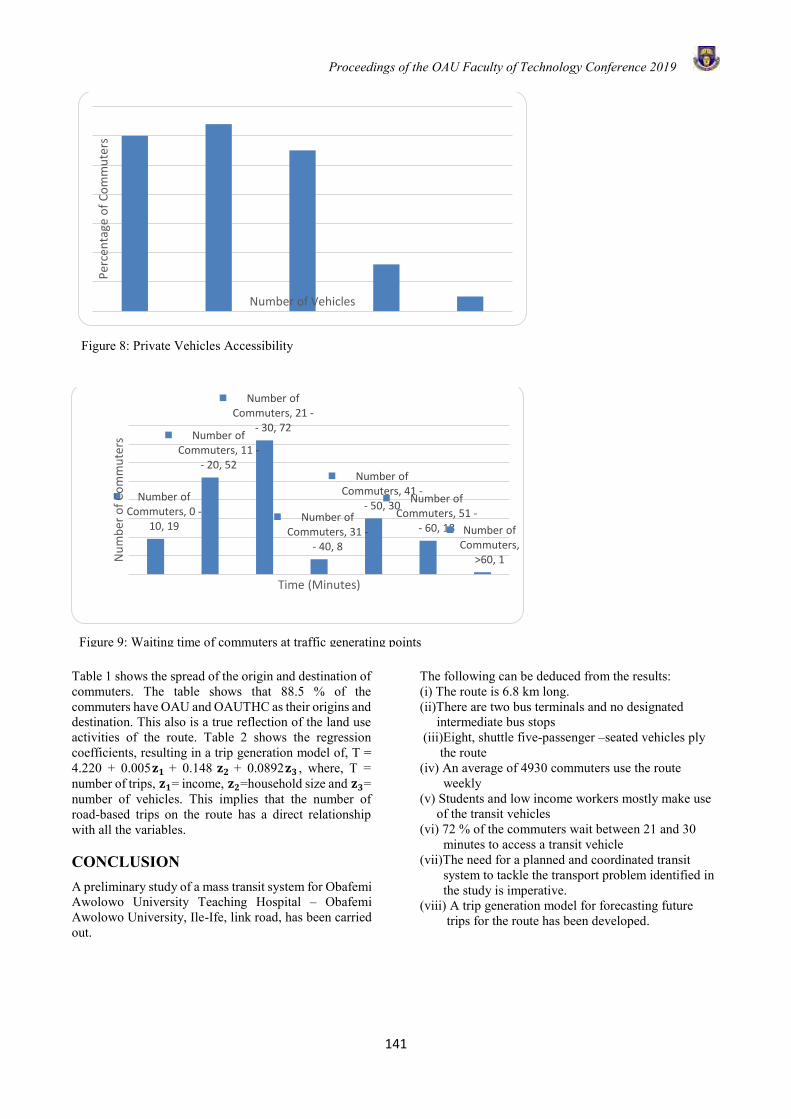
Proceedings of the OAU Faculty of Technology Conference 2019
141
Table 1 shows the spread of the origin and destination of commuters. The table shows that 88.5 % of the commuters have OAU and OAUTHC as their origins and destination. This also is a true reflection of the land use activities of the route. Table 2 shows the regression coefficients, resulting in a trip generation model of, T = 4.220 + 0.005𝐳𝟏 + 0.148 𝐳𝟐 + 0.0892𝐳𝟑 , where, T = number of trips, 𝐳𝟏= income, 𝐳𝟐=household size and 𝐳𝟑= number of vehicles. This implies that the number of road-based trips on the route has a direct relationship with all the variables. CONCLUSION A preliminary study of a mass transit system for Obafemi Awolowo University Teaching Hospital – Obafemi Awolowo University, Ile-Ife, link road, has been carried out.
The following can be deduced from the results: (i) The route is 6.8 km long. (ii)There are two bus terminals and no designated intermediate bus stops (iii)Eight, shuttle five-passenger –seated vehicles ply the route (iv) An average of 4930 commuters use the route weekly (v) Students and low income workers mostly make use of the transit vehicles (vi) 72 % of the commuters wait between 21 and 30 minutes to access a transit vehicle (vii)The need for a planned and coordinated transit system to tackle the transport problem identified in the study is imperative. (viii) A trip generation model for forecasting future trips for the route has been developed.
Per
cen
tage
of
Co
mm
ute
rs
Number of Vehicles
Number of Commuters, 0 -
10, 19
Number of Commuters, 11 -
- 20, 52
Number of Commuters, 21 -
- 30, 72
Number of Commuters, 31 -
- 40, 8
Number of Commuters, 41 -
- 50, 30Number of
Commuters, 51 -- 60, 18 Number of
Commuters, >60, 1N
um
ber
of
Co
mm
ute
rs
Time (Minutes)
Figure 8: Private Vehicles Accessibility
Figure 9: Waiting time of commuters at traffic generating points
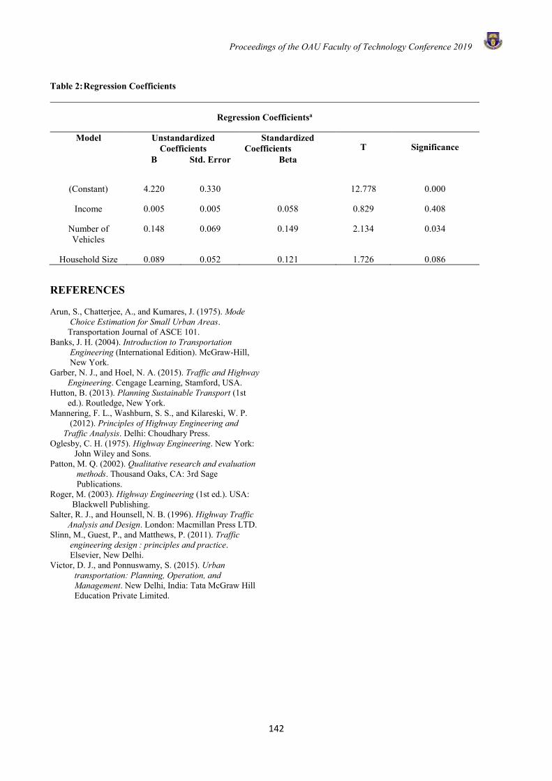
Proceedings of the OAU Faculty of Technology Conference 2019
142
Table 2: Regression Coefficients
Regression Coefficientsa
Model Unstandardized Coefficients
Standardized Coefficients T Significance
B Std. Error Beta
(Constant) 4.220 0.330 12.778 0.000
Income 0.005 0.005 0.058 0.829 0.408
Number of Vehicles
0.148 0.069 0.149 2.134 0.034
Household Size 0.089 0.052 0.121 1.726 0.086
REFERENCES Arun, S., Chatterjee, A., and Kumares, J. (1975). Mode Choice Estimation for Small Urban Areas. Transportation Journal of ASCE 101. Banks, J. H. (2004). Introduction to Transportation Engineering (International Edition). McGraw-Hill, New York. Garber, N. J., and Hoel, N. A. (2015). Traffic and Highway Engineering. Cengage Learning, Stamford, USA. Hutton, B. (2013). Planning Sustainable Transport (1st ed.). Routledge, New York. Mannering, F. L., Washburn, S. S., and Kilareski, W. P. (2012). Principles of Highway Engineering and Traffic Analysis. Delhi: Choudhary Press. Oglesby, C. H. (1975). Highway Engineering. New York: John Wiley and Sons. Patton, M. Q. (2002). Qualitative research and evaluation methods. Thousand Oaks, CA: 3rd Sage Publications. Roger, M. (2003). Highway Engineering (1st ed.). USA: Blackwell Publishing. Salter, R. J., and Hounsell, N. B. (1996). Highway Traffic Analysis and Design. London: Macmillan Press LTD. Slinn, M., Guest, P., and Matthews, P. (2011). Traffic engineering design : principles and practice. Elsevier, New Delhi. Victor, D. J., and Ponnuswamy, S. (2015). Urban transportation: Planning, Operation, and Management. New Delhi, India: Tata McGraw Hill Education Private Limited.
Proceedings of the OAU Faculty of Technology Conference 2019
143
ASSESSMENT OF WATER QUALITY INDEX OF GROUNDWATER RESOURCES IN IWO LOCAL GOVERNMENT AREA, OSUN STATE,
NIGERIA
Y. O. Adetona1,* and K. T. Oladepo1 1Department of Civil Engineering,
Obafemi Awolowo University, Ile-Ife, Nigeria. *Email of Corresponding Author: [email protected]
ABSTRACT
This study assessed the groundwater quality of thirty (30) selected wells and boreholes in Iwo Local Government Area, Osun State, Nigeria. Groundwater sources were randomly stratified and identified according to the fifteen (15) political wards using hand-held GPS equipment. The selected sources were sampled for two (2) seasons, during rainy season (October) and dry season (January) to determine water quality. The physico-chemical parameters of the water samples determined are temperature, turbidity, total suspended solids, pH, electrical conductivity, total dissolved solids, total alkalinity, total hardness, chloride, sulphate, nitrate, phosphate, magnesium, calcium, iron, zinc, lead, manganese, cadmium, and chromium. While the microbiological parameter determined is total coliform count. The results showed that total hardness, calcium, cadmium, sulphate and phosphate had mean values for rainy and dry seasons above the acceptable values; their mean values in mg/l for rainy season were 252.933, 98.267, 0.018, 305.119 and 1.762, respectively, while their values for dry season were 299.633, 115.831, 0.020, 285.695 and 1.705, respectively. The Water Quality Index (WQI) values showed that 30 % of the selected groundwater sources were fit for consumption while 60 % were slightly less potable and 10 % were unfit for drinking during rainy season. During the dry season, 50 % of the groundwater sources were fit for consumption, 40 % were slightly less potable and 10 % were unfit for consumption. The less potable sources of water supply should be subjected to water treatment.
Keywords: Contamination, drinking, potable water, water supply, treatment INTRODUCTION Water is basic for the survival of every living thing. It is also vital for economic and industrial developments. The population grows quickly in both developed and developing countries. This makes water an essential and valuable asset. It is needed domestically for drinking, agriculturally for irrigation and industrially for the production of goods. It is essential to check the quantity and quality of water aimed at residential, agricultural and industrial purposes. WHO (2017) stated that the provision of potable water is part of the Sustainable Development Goals (SDGs).
There are several major sources of water supply and these include groundwater and surface water. The groundwater plays a very significant role in meeting the ever increasing water demands from the residential, agricultural and industrial regions. Accessing water from underground sources involve technological efforts, such as sinking of wells and boreholes. Surface water however requires more treatment operations for its potability, because it gets contaminated easily due to increasing anthropogenic activities (Dohare et al., 2014). Nas (2009) reported that shortage supply of quality surface water due to rapid industrialization and population has amplified groundwater usage.
Recently, groundwater sources are under the risk of degradation in both quantity and quality in many parts of the world, especially in Nigeria (Adegbola and Adewoye, 2012a). Large quantities of human and industrial wastes are discharged into the environment, which cause serious threat to the groundwater (Adegbola and Adewoye, 2012b). These wastes eventually infiltrate the groundwater and their concentrations in the groundwater are enhanced by continuous discharge of wastes, coupled with some other environmental factors. According to (Munna et al., 2015), excessive pumping and unscientific management of aquifers are also accountable for deterioration of groundwater quality.
Generally, contaminations in built-up areas of Nigeria are anthropogenic. This is as a result of discharged effluents and untreated wastes, especially in Osun State, Nigeria (Jeje and Oladepo, 2014; Atobatele and Olutona, 2013). Menaces from water borne diseases are obviously public health distress in Iwo Local Government Area (Ogunbode et al., 2016). Water supply for domestic and industrial use should be free from disease-causing organisms and other matters which are unacceptable to the final consumers. This is because contaminated groundwater makes a negative impact to public health. In order to safeguard the public health, rigorous sampling and analysis of groundwater samples to assess water quality represent the major purpose of a
Proceedings of the OAU Faculty of Technology Conference 2019
144
monitoring program (Ahmed, 2017). The measurement of the type and level of contaminants present in a sample is generally referred to as water quality assessment.
Water quality index is an essential tool used to derive information about quality of any source of water supply (Herojeet et al., 2016). It is a technique which derives simple index by summarizing various groundwater quality parameters and serves as a useful tool in water quality management and control. The highly recommended water quality index established by various agencies and departments are the Washington State Water Quality Index, Taiwan Water Quality Index, Canadian Water Quality Index, Colombia Water Quality Index, Florida Stream Water Quality Index, French Creek Quality Index, France Water Quality Index, Malaysian Water Quality Index, Oregon Water Quality Index and British Colombia Water Act Quality Index (Mahapatra et al., 2012).
MATERIALS AND METHODS Study Area Iwo local Government Area is one of the 30 Local Government Areas in Osun State and Iwo is the administrative headquarter of Iwo Local Government Area of Osun State in the Southwestern geopolitical zone of Nigeria. It is divided into five quarters namely; Isale Oba, Molete, Oke Adan, Gidigbo and Oke Oba (Ogunbode et al., 2016). These are further subdivided into 15 political wards. The local government encompasses rural, agricultural and urban regions. The urban region forms Iwo town, which is bounded by Latitudes 07o38’ N to 07040’ N and Longitude 004009’ E to 004o11’ E.
The town has an area of 245 km2 with a population of 191,348 (National Population Commission, 2006). It is a nodal town from which towns such as Ibadan, Ile-Ogbo and Ede can readily be accessed. However, the study area shares boundaries with Aiyedire and Ola Oluwa Local Government Areas in Osun State. It also shares boundaries with Lagelu, Akinyele, Afijio and Oyo East in Oyo State. The study area is endowed with two rivers namely river Oba and river Aiba. River Aiba on latitude 07o37’41.0’’N is located at the north-eastern part of the study area, was dammed and named Aiba reservoir for public water supply.
It is a man-made lake located in Iwo city in the southwestern part of Nigeria. Aiba water reservoir located within government forest reservation area in the town serves as the major source of potable water in Iwo. Unfortunately, there is an inadequate supply of potable water from the water works, due to poor management and increase in the population of the area. This led to the exploitation of underground water sources in the town.
The mean annual rainfall varies from 1500 mm in the southern part of Nigeria to 3000 mm (Ogunbode et al., 2016; Olutona et al., 2012). Mean maximum ambient temperature values range between 33.84 oC in February
and 28.8 oC in August, while mean minimum temperatures range between 25.18 oC in March and 23.0 oC in August. Higher temperatures are mostly recorded at the peak of the dry season, while lower temperatures are recorded in the rainy season.
Collection of Samples Water samples were collected for water quality and bacteriological studies from 30 locations including boreholes, hand pump and shallow wells within Iwo local Government Area as shown in Table 1. The sampling was designed to target the population demanding groundwater majorly for domestic purpose. Therefore groundwater sources were randomly stratified and identified according to the 15 political wards using hand-held Global Positioning System (GPS) equipment. Most of the wells were covered in the urban region, while those located at rural regions were unlined and hand pump. Sampling was done during the rainy season (October) and also during dry season (January).
Analysis of Water Samples Physical, chemical and microbiological parameters such as temperature, turbidity, pH, electrical conductivity, total suspended solids, total dissolved solids, total alkalinity, total hardness, chloride, sulphate, nitrate, phosphate, magnesium, calcium, iron, zinc, lead, manganese, cadmium, chromium and total coliform were selected in line with (Olutona et al., 2012) and (Ogunbode et al., 2016).
The pH of water samples were measured in-situ, using a pH meter. Temperature was measured at the sampling points using a mercury thermometer with an accuracy of 0.1 oC, at 25 oC. Electrical conductivities of the water samples were determined using platinum electrode conductivity meter. Total dissolved solid was determined by using total dissolved solid meter. The quantity of chloride present in the water samples was determined by titration using standard silver nitrate. Hardness was determined by standard Ethylene Diamine Tetra-acetic Acid (EDTA) titration method.
Sulphate, nitrate and phosphate concentrations of the water samples were determined using UV-Spectrophotometer. Complexometric titration method was used to find the quantity of calcium of the hardness of water by titrating the water sample with a standard EDTA of known concentration and volume. Magnesium was determined by calculating the difference between total hardness and calcium hardness as CaCO3 equivalent. The result was multiplied by mass ratio of magnesium (0.243).

Proceedings of the OAU Faculty of Technology Conference 2019
145
Table 1: Location of Sampled Groundwater Sources
S/N Political Ward Latitude Longitude GL(m) 1 Isale Oba Ward 01A 07037′32.6″ 04010′38.7″ 237 2 Isale Oba Ward 01B 07037′46.6″ 04010′43.9″ 249 3 Isale Oba Ward 02A 07037′37.2″ 04010′52.7″ 237 4 Isale Oba Ward 02B 07037′45.5″ 04010′22.5″ 249 5 Isale Oba Ward 03A 07037′52.7″ 04012′02.2″ 245 6 Isale Oba Ward 03B 07037′49.2″ 04011′33.4″ 242 7 Isale Oba Ward 04A 07037′36.5″ 04010′15.8″ 241 8 Isale Oba Ward 04B 07036′55.6″ 04011′26.4″ 242 9 Molete Ward 05A 07037′58.8″ 04011′01.3″ 250 10 Molete Ward 05B 07038′02.4″ 04010′49.6″ 259 11 Molete Ward 06A 07038′11.7″ 04011′14.8″ 246 12 Molete Ward 06B 07038′42.5″ 04012′42.5″ 254 13 Molete Ward 07A 07038′35.0″ 04011′10.9″ 260 14 Molete Ward 07B 07038′35.1″ 04011′10.8″ 260 15 Oke Adan Ward 08A 07038′10.6″ 04010′54.7″ 249 16 Oke Adan Ward 08B 07038′12.0″ 04010′57.5″ 255 17 Oke Adan Ward 09A 07038′08.7″ 04010′50.2″ 253 18 Oke Adan Ward 09B 07038′13.9″ 04010′43.3″ 252 19 Oke Adan Ward 10A 07039′16.4″ 04010′38.9″ 269 20 Oke Adan Ward 10B 07039′32.9″ 04011′44.3″ 255 21 Gidigbo Ward 11A 07037′45.7″ 04010′08.3″ 243 22 Gidigbo Ward 11B 07038′20.9″ 04009′49.9″ 248 23 Gidigbo Ward 12A 07037′59.3″ 04010′35.6″ 255 24 Gidigbo Ward 12B 07038′41.4″ 04009′57.1″ 248 25 Gidigbo Ward 13A 07037′39.2″ 04009′50.1″ 225 26 Gidigbo Ward 13B 07038′00.8″ 04010′08.2″ 237 27 Oke Oba Ward 14A 07038′29.6″ 04003′23.7″ 264 28 Oke Oba Ward 14B 07036′58.0″ 04005′50.0″ 235 29 Oke Oba Ward 15A 07034′30.7″ 04006′52.7″ 227 30 Oke Oba Ward 15B 07033′49.9″ 04008′02.7″ 225
The alkalinity of the water samples were determined by titrating 100 ml of the samples with 0.2 N solution of sulphuric acid using phenolphthalein and mixed indicators as indicators. Total suspended solid was measured gravimetrically after drying in an oven at 105 oC and cooled to room temperature in a desiccator. Electronic turbid meter with scattered-light detectors was used for turbidity measurement after calibrating the instrument with distilled water.
The total coliform in the water samples were obtained using the membrane-filtration method. The heavy metals in the samples were analyzed using Atomic Absorption Spectrophotometer (AAS) which makes use of flame as the atomizer. In order to obtain accurate result, 100 ml of sampled water were digested with 10 ml concentrated nitric acid.
The solution was heated for a period of 30 minutes, cooled and transferred to a 100 ml beaker which was filled up to 100 ml mark with distilled water.
Calculation of Water Quality Index According to Verma et al. (2013), water quality index of a source of water supply are mostly calculated using the following equations:
𝑊𝑄𝐼 = ∑ 𝑊𝑖 × 𝑄𝑖𝑛𝑖=1 (1)
𝑊𝑖 = 𝐾
𝑆𝑖 (2)
𝐾 = [1
∑1
𝑆𝑖
𝑛𝑛=𝑖
] (3)
𝑄𝑖 = [(𝑉𝑎− 𝑉𝑖)
(𝑉𝑠− 𝑉𝑖) × 100] (4)
where, WQI = Water Quality Index Qi = Quality rating Wn = Unit weight Va = Measured value of water quality parameter Vi = Ideal Value of the parameter. (pH = 7, other parameters = 0) Vs = Standard value of the water quality parameter
Sn = Acceptable value of water quality parameter
from standards.
K = Proportionality constant
Si = Individual standard value for water quality
parameter
N = number of parameters
Based on the water quality index, quality of groundwater supply from sampling points were categorized into unfit for drinking (> 100), very poor (76 – 100), poor (51 – 75), good (26 – 50) and excellent (0 – 25) (Oko et al., 2014). Turbidity, chloride, nitrate, pH, hardness, total dissolved solids and electrical conductivity were the seven selected parameters used for water quality index.
RESULTS AND DISCUSSION Rainy season The mean temperature for the sampled wells during rainy season was 27.48 oC, clearly above the guideline value of 25 oC. The pH of the water samples ranged from 5.6 to 8.5 and had a mean of 7.07 which was within the World Health Organization (WHO) guideline value of 6.5 – 8.5. The mean electrical conductivity (568.60 μS/cm) was below the guideline value of 1,000 μS/cm. The mean total dissolved solid (330.57 mg/l) was below the guideline value of 500 mg/l. The mean value of chloride (67.13 mg/l) was below the guideline value of 250 mg/l.
The mean total alkalinity (120.57 mg/l) was below the guideline value of 200 mg/l. The mean total suspended solid (180 mg/l) was below the guideline value of 250 mg/l. The mean turbidity was 3.90 Nephelometric Turbidity Unit (NTU) was below the guideline value of 5 NTU. The mean total hardness (252.93 mg/l) was above the guideline value of 150 mg/l. The mean calcium (98.27 mg/l) was above the guideline value of 75 mg/l. The mean magnesium (1.91 mg/l) was below the guideline value of 50 mg/l.
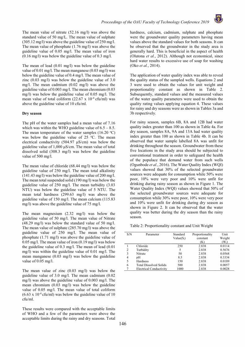
Proceedings of the OAU Faculty of Technology Conference 2019
146
The mean value of nitrate (52.16 mg/l) was above the standard value of 50 mg/L. The mean value of sulphate (305.12 mg/l) was above the guideline value of 250 mg/l. The mean value of phosphate (1.76 mg/l) was above the guideline value of 0.05 mg/l. The mean value of iron (0.16 mg/l) was below the guideline value of 0.3 mg/l.
The mean of lead (0.01 mg/l) was below the guideline value of 0.01 mg/l. The mean manganese (0.03 mg/l) was below the guideline value of 0.4 mg/l. The mean value of zinc (0.03 mg/l) was below the guideline value of 3.0 mg/l. The mean cadmium (0.02 mg/l) was above the guideline value of 0.003 mg/l. The mean chromium (0.03 mg/l) was below the guideline value of 0.05 mg/l. The mean value of total coliform (22.67 x 10⁻⁴ cfu/ml) was above the guideline value of 10 cfu/ml.
Dry season
The pH of the water samples had a mean value of 7.16 which was within the WHO guideline value of 6.5 – 8.5. The mean temperature of the water samples (16.20 oC) was below the guideline value of 25 oC. The mean electrical conductivity (504.97 μS/cm) was below the guideline value of 1,000 μS/cm. The mean value of total dissolved solid (308.3 mg/l) was below the guideline value of 500 mg/l.
The mean value of chloride (68.44 mg/l) was below the guideline value of 250 mg/l. The mean total alkalinity (141.43 mg/l) was below the guideline value of 200 mg/l. The mean total suspended solid (190 mg/l) was below the guideline value of 250 mg/l. The mean turbidity (3.03 NTU) was below the guideline value of 5 NTU. The mean total hardness (299.63 mg/l) was above the guideline value of 150 mg/l. The mean calcium (115.83 mg/l) was above the guideline value of 75 mg/l.
The mean magnesium (2.32 mg/l) was below the guideline value of 50 mg/l. The mean value of Nitrate (48.29 mg/l) was below the standard value of 50 mg/l. The mean value of sulphate (285.70 mg/l) was above the guideline value of 250 mg/l. The mean value of phosphate (1.71 mg/l) was above the guideline value of 0.05 mg/l. The mean value of iron (0.19 mg/l) was below the guideline value of 0.3 mg/l. The mean of lead (0.01 mg/l) was within the guideline value of 0.01 mg/l. The mean manganese (0.03 mg/l) was below the guideline value of 0.05 mg/l.
The mean value of zinc (0.03 mg/l) was below the guideline value of 3.0 mg/l. The mean cadmium (0.02 mg/l) was above the guideline value of 0.003 mg/l. The mean chromium (0.03 mg/l) was below the guideline value of 0.05 mg/l. The mean value of total coliform (6.63 x 10⁻⁴ cfu/ml) was below the guideline value of 10 cfu/ml.
These results were compared with the acceptable limits of WHO and a few of the parameters were above the acceptable limits during the rainy and dry seasons. Total
hardness, calcium, cadmium, sulphate and phosphate were the groundwater quality parameters having mean values above the standard values for both seasons. It can be observed that the groundwater in the study area is generally hard. This is beneficial in the aspect of health (Olutona et al., 2012). Although not economical, since hard water results to excessive use of soap for washing (Oko et al., 2014).
The application of water quality index was able to reveal the quality status of the sampled wells. Equations 2 and 3 were used to obtain the values for unit weight and proportionality constant as shown in Table 2. Subsequently, standard values and the measured values of the water quality parameters were used to obtain the quality rating values applying equation 4. These values for rainy and dry seasons were as shown in Tables 3a and 3b respectively.
For rainy season, samples 6B, 8A and 12B had water quality index greater than 100 as shown in Table 4a. For dry season, samples 8A, 9A and 13A had water quality index greater than 100 as shown in Table 4b. It can be observed that water sample labelled 8A was unfit for drinking throughout the season. Groundwater from these five locations in the study area should be subjected to conventional treatment in order to safeguard the health of the populace that demand water from such wells (Ogunbode et al., 2016). The Water Quality Index (WQI) values showed that 30% of the selected groundwater sources were adequate for consumption while 50% were poor, 10% were very poor and 10% were unfit for drinking during rainy season as shown in Figure 1. The Water Quality Index (WQI) values showed that 50% of the selected groundwater sources were adequate for consumption while 30% were poor, 10% were very poor and 10% were unfit for drinking during dry season as shown in Figure 2. It can be observed that the water quality was better during the dry season than the rainy season.
Table 2: Proportionality constant and Unit Weight
S/N Parameter Standard Value(Si)
Proportionality constant
(K)
Unit Weight
(Wi) 1 Chloride 250 2.838 0.0114 2 Turbidity 5 2.838 0.5676 3 Nitrate 50 2.838 0.0568 4 pH 8.5 2.838 0.3334 5 Hardness 150 2.838 0.0189 6 Total Dissolved Solids 500 2.838 0.0057 7 Electrical Conductivity 1000 2.838 0.0028
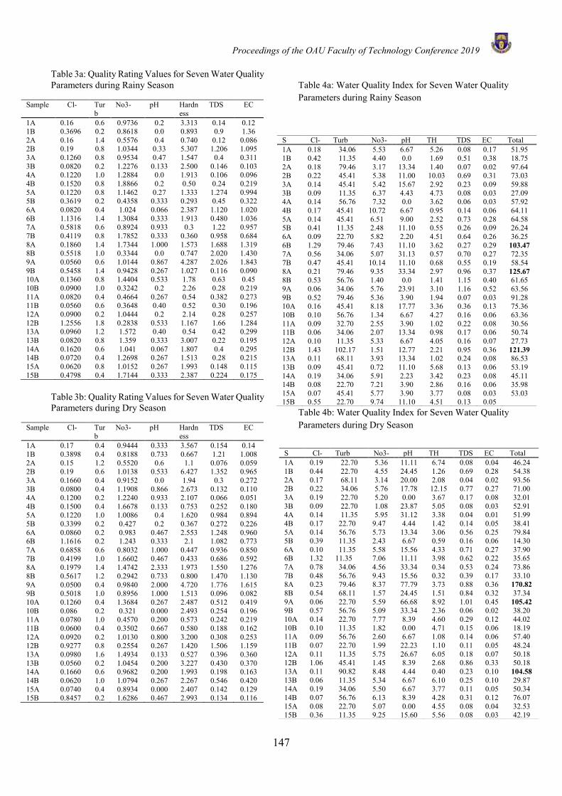
Proceedings of the OAU Faculty of Technology Conference 2019
147
Table 3a: Quality Rating Values for Seven Water Quality Parameters during Rainy Season
Sample Cl- Turb
No3- pH Hardness
TDS EC
1A 0.16 0.6 0.9736 0.2 3.313 0.14 0.12 1B 0.3696 0.2 0.8618 0.0 0.893 0.9 1.36 2A 0.16 1.4 0.5576 0.4 0.740 0.12 0.086 2B 0.19 0.8 1.0344 0.33 5.307 1.206 1.095 3A 0.1260 0.8 0.9534 0.47 1.547 0.4 0.311 3B 0.0820 0.2 1.2276 0.133 2.500 0.146 0.103 4A 0.1220 1.0 1.2884 0.0 1.913 0.106 0.096 4B 0.1520 0.8 1.8866 0.2 0.50 0.24 0.219 5A 0.1220 0.8 1.1462 0.27 1.333 1.274 0.994 5B 0.3619 0.2 0.4358 0.333 0.293 0.45 0.322 6A 0.0820 0.4 1.024 0.066 2.387 1.120 1.020 6B 1.1316 1.4 1.3084 0.333 1.913 0.480 1.036 7A 0.5818 0.6 0.8924 0.933 0.3 1.22 0.957 7B 0.4119 0.8 1.7852 0.333 0.360 0.958 0.684 8A 0.1860 1.4 1.7344 1.000 1.573 1.688 1.319 8B 0.5518 1.0 0.3344 0.0 0.747 2.020 1.430 9A 0.0560 0.6 1.0144 0.867 4.287 2.026 1.843 9B 0.5458 1.4 0.9428 0.267 1.027 0.116 0.090 10A 0.1360 0.8 1.4404 0.533 1.78 0.63 0.45 10B 0.0900 1.0 0.3242 0.2 2.26 0.28 0.219 11A 0.0820 0.4 0.4664 0.267 0.54 0.382 0.273 11B 0.0560 0.6 0.3648 0.40 0.52 0.30 0.196 12A 0.0900 0.2 1.0444 0.2 2.14 0.28 0.257 12B 1.2556 1.8 0.2838 0.533 1.167 1.66 1.284 13A 0.0960 1.2 1.572 0.40 0.54 0.42 0.299 13B 0.0820 0.8 1.359 0.333 3.007 0.22 0.195 14A 0.1620 0.6 1.041 0.067 1.807 0.4 0.295 14B 0.0720 0.4 1.2698 0.267 1.513 0.28 0.215 15A 0.0620 0.8 1.0152 0.267 1.993 0.148 0.115 15B 0.4798 0.4 1.7144 0.333 2.387 0.224 0.175
Table 3b: Quality Rating Values for Seven Water Quality Parameters during Dry Season
Sample Cl- Turb
No3- pH Hardness
TDS EC
1A 0.17 0.4 0.9444 0.333 3.567 0.154 0.14 1B 0.3898 0.4 0.8188 0.733 0.667 1.21 1.008 2A 0.15 1.2 0.5520 0.6 1.1 0.076 0.059 2B 0.19 0.6 1.0138 0.533 6.427 1.352 0.965 3A 0.1660 0.4 0.9152 0.0 1.94 0.3 0.272 3B 0.0800 0.4 1.1908 0.866 2.673 0.132 0.110 4A 0.1200 0.2 1.2240 0.933 2.107 0.066 0.051 4B 0.1500 0.4 1.6678 0.133 0.753 0.252 0.180 5A 0.1220 1.0 1.0086 0.4 1.620 0.984 0.894 5B 0.3399 0.2 0.427 0.2 0.367 0.272 0.226 6A 0.0860 0.2 0.983 0.467 2.553 1.248 0.960 6B 1.1616 0.2 1.243 0.333 2.1 1.082 0.773 7A 0.6858 0.6 0.8032 1.000 0.447 0.936 0.850 7B 0.4199 1.0 1.6602 0.467 0.433 0.686 0.592 8A 0.1979 1.4 1.4742 2.333 1.973 1.550 1.276 8B 0.5617 1.2 0.2942 0.733 0.800 1.470 1.130 9A 0.0500 0.4 0.9840 2.000 4.720 1.776 1.615 9B 0.5018 1.0 0.8956 1.000 1.513 0.096 0.082 10A 0.1260 0.4 1.3684 0.267 2.487 0.512 0.419 10B 0.086 0.2 0.321 0.000 2.493 0.254 0.196 11A 0.0780 1.0 0.4570 0.200 0.573 0.242 0.219 11B 0.0600 0.4 0.3502 0.667 0.580 0.188 0.162 12A 0.0920 0.2 1.0130 0.800 3.200 0.308 0.253 12B 0.9277 0.8 0.2554 0.267 1.420 1.506 1.159 13A 0.0980 1.6 1.4934 0.133 0.527 0.396 0.360 13B 0.0560 0.2 1.0454 0.200 3.227 0.430 0.370 14A 0.1660 0.6 0.9682 0.200 1.993 0.198 0.163 14B 0.0620 1.0 1.0794 0.267 2.267 0.546 0.420 15A 0.0740 0.4 0.8934 0.000 2.407 0.142 0.129 15B 0.8457 0.2 1.6286 0.467 2.993 0.134 0.116
Table 4a: Water Quality Index for Seven Water Quality Parameters during Rainy Season
Table 4b: Water Quality Index for Seven Water Quality Parameters during Dry Season
S Cl- Turb No3- pH TH TDS EC Total 1A 0.19 22.70 5.36 11.11 6.74 0.08 0.04 46.24 1B 0.44 22.70 4.55 24.45 1.26 0.69 0.28 54.38 2A 0.17 68.11 3.14 20.00 2.08 0.04 0.02 93.56 2B 0.22 34.06 5.76 17.78 12.15 0.77 0.27 71.00 3A 0.19 22.70 5.20 0.00 3.67 0.17 0.08 32.01 3B 0.09 22.70 1.08 23.87 5.05 0.08 0.03 52.91 4A 0.14 11.35 5.95 31.12 3.38 0.04 0.01 51.99 4B 0.17 22.70 9.47 4.44 1.42 0.14 0.05 38.41 5A 0.14 56.76 5.73 13.34 3.06 0.56 0.25 79.84 5B 0.39 11.35 2.43 6.67 0.59 0.16 0.06 14.30 6A 0.10 11.35 5.58 15.56 4.33 0.71 0.27 37.90 6B 1.32 11.35 7.06 11.11 3.98 0.62 0.22 35.65 7A 0.78 34.06 4.56 33.34 0.34 0.53 0.24 73.86 7B 0.48 56.76 9.43 15.56 0.32 0.39 0.17 33.10 8A 0.23 79.46 8.37 77.79 3.73 0.88 0.36 170.82 8B 0.54 68.11 1.57 24.45 1.51 0.84 0.32 37.34 9A 0.06 22.70 5.59 66.68 8.92 1.01 0.45 105.42 9B 0.57 56.76 5.09 33.34 2.36 0.06 0.02 38.20 10A 0.14 22.70 7.77 8.39 4.60 0.29 0.12 44.02 10B 0.10 11.35 1.82 0.00 4.71 0.15 0.06 18.19 11A 0.09 56.76 2.60 6.67 1.08 0.14 0.06 57.40 11B 0.07 22.70 1.99 22.23 1.10 0.11 0.05 48.24 12A 0.11 11.35 5.75 26.67 6.05 0.18 0.07 50.18 12B 1.06 45.41 1.45 8.39 2.68 0.86 0.33 50.18 13A 0.11 90.82 8.48 4.44 0.40 0.23 0.10 104.58 13B 0.06 11.35 5.34 6.67 6.10 0.25 0.10 29.87 14A 0.19 34.06 5.50 6.67 3.77 0.11 0.05 50.34 14B 0.07 56.76 6.13 8.39 4.28 0.31 0.12 76.07 15A 0.08 22.70 5.07 0.00 4.55 0.08 0.04 32.53 15B 0.36 11.35 9.25 15.60 5.56 0.08 0.03 42.19
S Cl- Turb No3- pH TH TDS EC Total 1A 0.18 34.06 5.53 6.67 5.26 0.08 0.17 51.95 1B 0.42 11.35 4.40 0.0 1.69 0.51 0.38 18.75 2A 0.18 79.46 3.17 13.34 1.40 0.07 0.02 97.64 2B 0.22 45.41 5.38 11.00 10.03 0.69 0.31 73.03 3A 0.14 45.41 5.42 15.67 2.92 0.23 0.09 59.88 3B 0.09 11.35 6.37 4.43 4.73 0.08 0.03 27.09 4A 0.14 56.76 7.32 0.0 3.62 0.06 0.03 57.92 4B 0.17 45.41 10.72 6.67 0.95 0.14 0.06 64.11 5A 0.14 45.41 6.51 9.00 2.52 0.73 0.28 64.58 5B 0.41 11.35 2.48 11.10 0.55 0.26 0.09 26.24 6A 0.09 22.70 5.82 2.20 4.51 0.64 0.26 36.25 6B 1.29 79.46 7.43 11.10 3.62 0.27 0.29 103.47 7A 0.56 34.06 5.07 31.13 0.57 0.70 0.27 72.35 7B 0.47 45.41 10.14 11.10 0.68 0.55 0.19 58.54 8A 0.21 79.46 9.35 33.34 2.97 0.96 0.37 125.67 8B 0.53 56.76 1.40 0.0 1.41 1.15 0.40 61.65 9A 0.06 34.06 5.76 23.91 3.10 1.16 0.52 63.56 9B 0.52 79.46 5.36 3.90 1.94 0.07 0.03 91.28 10A 0.16 45.41 8.18 17.77 3.36 0.36 0.13 75.36 10B 0.10 56.76 1.34 6.67 4.27 0.16 0.06 63.36 11A 0.09 32.70 2.55 3.90 1.02 0.22 0.08 30.56 11B 0.06 34.06 2.07 13.34 0.98 0.17 0.06 50.74 12A 0.10 11.35 5.33 6.67 4.05 0.16 0.07 27.73 12B 1.43 102.17 1.51 12.77 2.21 0.95 0.36 121.39 13A 0.11 68.11 3.93 13.34 1.02 0.24 0.08 86.53 13B 0.09 45.41 0.72 11.10 5.68 0.13 0.06 53.19 14A 0.19 34.06 5.91 2.23 3.42 0.23 0.08 45.11 14B 0.08 22.70 7.21 3.90 2.86 0.16 0.06 35.98 15A 0.07 45.41 5.77 3.90 3.77 0.08 0.03 53.03 15B 0.55 22.70 9.74 11.10 4.51 0.13 0.05
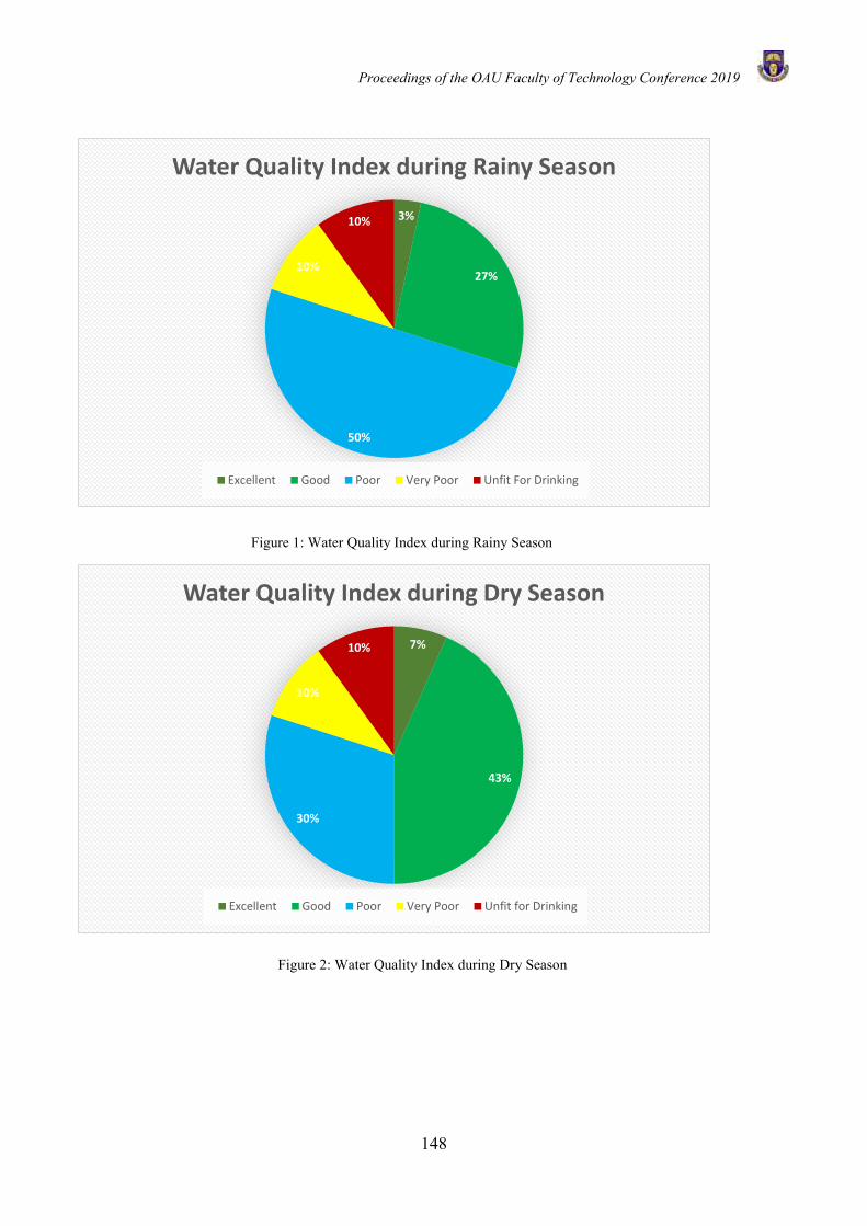
Proceedings of the OAU Faculty of Technology Conference 2019
148
Figure 3: Water Quality Index for the Study Area during Dry Seas
3%
27%
50%
10%
10%
Water Quality Index during Rainy Season
Excellent Good Poor Very Poor Unfit For Drinking
7%
43%
30%
10%
10%
Water Quality Index during Dry Season
Excellent Good Poor Very Poor Unfit for Drinking
Figure 1: Water Quality Index during Rainy Season
Figure 2: Water Quality Index during Dry Season
Proceedings of the OAU Faculty of Technology Conference 2019
149
CONCLUSION Five out of the thirty sampled groukndwater sources were confirmed unfit for drinking during both rainy and dry seasons. These were based on the results from the water quality index, which is useful for effective management by the societal policymakers (Acharya et al., 2018). These wells had water quality index greater than 100 (Oko et al., 2014). These wells should be subjected to water treatment processes, such as that used in Obafemi Awolowo University ozonized bottled water production system (Oladepo et al., 2012). While others were either poor or good for drinking, which can be subjected to slight or no conventional treatment respectively.
Water supply for domestic and industrial use should be free from disease-causing organisms and other matters which are unacceptable to the final consumers (Adegbola and Adewoye, 2012b). Therefore, periodical assessment of physical, chemical and microbial analysis of groundwater in Iwo Local Government Area is recommended. This assessment will aid early identification of any potential future degradation of the groundwater parameters which were below and within the acceptable limits. There should be frequent public awareness by the local government officials about the role of individuals to protect groundwater from residential, agricultural and industrial waste contaminations.
REFERENCES Acharya, S., Sharma, S. K., and Khandegar, V.,
Assessment of groundwater quality by Water Quality Indices for Irrigation and drinking in South West Delhi, India. Data in Brief, 18: 1-5, 2018.
Adegbola, A. A., and Adewoye, A. O., On Investigating Pollution of Groundwater from Atenda Abattoir. International Journal of Modern Engineering Research, 2 (9): 1-17, 2012a.
Adegbola, A. A., and Adewoye, A. O., Impact Assessment of Selected Pollution Sources on Groundwater Quality in Wells in Gambari Community , Ogbomoso, Nigeria. International Journal of Modern Engineering Research, 2(5): 3118–3122, 2012b.
Ahmed, S. S., Assessment of Groundwater Quality Parameters Using Multivariate Statistics- A Case Study of Majmaah, 5(2): 40, 2017.
Atobatele, E. O., and Olutona, G. O., Spatio-seasonal physico-chemistry of Aiba stream, Iwo, Nigeria. 12(14): 1630–1635, 2013.
Dohare, D., Deshpande, S., and Kotiya, A., Analysis of Ground Water Quality Parameters : A Review.
Research Journal of Engineering Sciences, 3(5): 26–31, 2014.
Herojeet, R., Rishi, M. S., Lata, R., and Sharma, R., Application of environmetrics statistical models and water quality index for groundwater quality characterization of alluvial aquifer of Nalagarh Valley, Himachal Pradesh, India. Sustainable Water Resources Management, Springer International Publishing, 2(1): 39–53, 2016.
Jeje, J. O., and Oladepo, K. T., Assessment of Heavy Metals of Boreholes and Hand Dug Wells in Ife North Local Government Area of Osun State , Nigeria. International Journal of Science and Technology, 3(4): 209–214, 2014.
Mahapatra, S. S., Sahu, M., Patel, R. K., and Panda, B. N., Prediction of Water Quality Using Principal Component Analysis. Water Qual Expo Health, 4: 93–104, 2012.
Munna, G., Nury, A. H., Islam, S., and Rahman, H., Spatial Distribution Analysis and Mapping of Groundwater Quality Parameters for the Sylhet City Corporation (SCC) Area Using GIS. Hydrology, 3(1): 1–10, 2015.
Nas, B., Geostatistical Approach to Assessment of Spatial Distribution of Groundwater Quality. Polish J. of Environ. Stud., 18(6): 1073–1082, 2009.
National Population Commission, Population Census Figure. Federal Republic of Nigeria, 2006.
Ogunbode, T. O., Akintunde, E. A., and Akinola, O. T., Assessment of Underground Water Quality and Pollution Sources Apportionment in a Growing Urban Centre in Osun State South Western Nigeria. European Journal of Geography, 7(3): 71–85, 2016.
Oko, O. J., Aremu, M. O., Odoh, R., Yebpella, G., and Shenge, G. A., Assessment of Water Quality Index of Borehole and Well Water in Wukari Town , Taraba State, Nigeria. Journal of Environmental and Earth Science, 4(5): 9, 2014.
Oladepo, K. T., Jeje, J. O., Ogedengbe, M. O., and Fadipe, O. O., Technical Assessment of a University-Based Ozone-Treated Bottled Water Production System. Transnational Journal of Science and Technology, 2(9): 31–46, 2012.

Proceedings of the OAU Faculty of Technology Conference 2019
150
Olutona, G. O., Akintunde, E. A., and Otolorin, J. A., Physico-chemical quality assessment of shallow well- waters in Iwo, southwestern Nigeria. Journal of Environmental Science and Water Resources, 1(6): 127–132, 2012.
Verma, A., Thakur, B., Katiyar, S., Singh, D., and Rai, M., Evaluation of ground water quality in Lucknow , Uttar Pradesh using remote sensing and geographic information systems (GIS). International Journal of Water Resources and Environmental Engineering, 5(2): 67–76, 2013.
WHO, Guidelines for drinking water quality: fourth edition incorporating the first addendum.Geneva, 2017.
Proceedings of the OAU Faculty of Technology Conference 2019
151
CHEMICAL AND SENSORY PROPERTIES OF PROBIOTICATED DRINKS FROM BLENDS OF AFRICAN YAM BEAN (AYB), SOYBEAN AND
COCONUT MILK ANALOGUES
A. V. Ikujenlola*, E. A. Adurotoye and H. A. Adeniran 1Department of Food Science and Technology, Obafemi Awolowo University, Ile-Ife, Nigeria.
*Email of Corresponding Author: [email protected]
ABSTRACT
This study assessed the physicochemical and sensory properties of ‘probiotic’ drink from blends of milk analogues from African yam bean (AYB), soybean (SM) and coconut (CM). Milk analogues were blended at ratios of 1:1:1, 3:1:1 and 5:1:1 (AYM: SM: CM) as samples A, B and C respectively. These samples were fermented for 24 h at 430C using Lactobacillus delbrueckii. The results showed that the fermented milk analogue of ratio 1:1:1 was the most acceptable in terms of sensory parameters. The pH of the milk analogues ranged from 5.07 to 5.85. The sample B1 (fermented (1:1:1) AYB: SM: CM) had a crude protein of 2.38%, potassium of 80.13 mg/100g, phytate of 2.85 mg/100g and saponin was 0.19 mg/100g. The study concluded that the sample with equal ratio of AYM, SM and CM adjudged the most acceptable by tasters.
Keywords: kunun zaki; milk analogues; phytate; reducing sugar INTRODUCTION Most probiotic foods in markets today are dairy based. The choice and preference of consumers tend towards foods that are supplemented with or replaced by plants. This is because plants have a minimal cholesterol contents and may serve as a relief for consumers who suffer from lactose intolerance. The increasing awareness of the interaction between diet and health has led to a high acceptance and craving for food and food products that boost health with respect to providing basic nutrients. This awareness has increased market demand particularly within children and other high-risk individuals for functional products containing probiotic bacteria. These have positive effect(s) on health and it is of consumers’ interest and attention. This is being promoted by health professionals (Yilmaz-Ersan and Kurdal, 2014). The term ‘probiotics’ originates from the Greek ‘Pro bios’ meaning ‘for life’ used to describe microorganisms that are responsible for the beneficial effects for humans and animals. These microbes contribute to intestinal microbial balance and contribute to maintaining sound health (Soccol et al., 2010). These beneficial microbes are majorly the strains of the genera Lactobacillus and Bifidobacterium, likewise strains of Bacillus, Pediococcus, and some yeast also perform these functions. All display a function in the protection of the organism against pathogens and also strengthen the host’s immune system (Soccol et al., 2010). Probiotics perform a key function in accelerating host immunity to colonization by exogenous, potentially pathogenic organisms. This is possible through different mechanisms such as production of lactic acid, hydrogen peroxide or acetic acid which accelerate the acidity of the
intestine and stops the reproduction of various pathogens (Hassan et al., 2013). Probiotics can be delivered in dairy and non-dairy products. Fermented dairy foods are the perfect conveyors for probiotics, which promote growth and enhance the thriving of these organisms. Of these foods, yoghurt is the most popular, and provides higher levels of protein, carbohydrate, calcium and certain B vitamins than milk (Yilmaz-Ersan and Kurdal, 2014). However, non- dairy fermented foods have also been produced mostly from underutilized and under-exploited plants. Adeniran et al. (2015) produced a probiotic drink from milk blends of AYB, soybean and coconut and determined the viability of the probiotic organisms in vitro. Osundahunsi et al. (2007) also determined the quality and acceptability of soy-yoghurt with different colours and fruit flavours. Ebhodaghe et al. (2012) assessed the physico-chemical characteristics, viability and inhibitory effect of Bifidobacteria in soymilk. These studies were limited to nutritional and effects of these probiotic drinks in vitro. Mbaeyi (2011) also produced a non-dairy probiotic yoghurt analogue from milk blends of soybean and ‘acha’ and determined the proximate and micronutrient composition. However, there is scanty information on the nutritional quality of the combination of African Yam Bean, soybean and coconut milk used as a probiotic drink. Therefore, this study is designed to produce and evaluate the chemical and sensory characteristics of probioticated drinks based on the combination of the underutilized crops of African Yam Bean (AYB), soybean and coconut. MATERIALS AND METHODS Materials The dried seeds of African Yam Bean (AYB), soybean and coconut drupes were collected from IAR&T, Apata,

Proceedings of the OAU Faculty of Technology Conference 2019
152
Ibadan, Nigeria. Lactobacillus delbrueckii characterized and identified from kununzaki drink produced in the Department of Food Science and Technology, OAU, Ile-Ife, Nigeria was used as the probiotic organism. The chemicals used were of analytical grade and were obtained from Sigma Adrich, USA. Methods Preparation of the vegetable extracts Milk extracts from the plant sources were obtained using the following procedures; Preparation of AYB milk analogue Seeds were examined and sorted to remove extraneous materials such as dirt, dust as well as shriveled and diseased (pest infested ones). The seeds were washed, soaked in warm water for 7 hours, drained and blanched for 5 mins at 100 oC, dehulled and milled with water (1:4) in a blender (Marlex, Excella model, India). The resulting slurry was filtered, allowed to stand for 5 mins and then boiled for 15 mins with constant stirring and rapid cooling (Aminigo et al., 2007). Preparation of soymilk Wholesome soybean seeds were soaked in warm water for 6 hours to give a bean:water ratio of 1:3. The seeds were drained, rinsed with water and blanched for 5 mins at 100 oC, dehulled and milled with water. The resulting slurry was filtered through a muslin cloth and the extract was boiled for 15 mins with constant stirring and rapid cooling (Udeozor, 2012). Preparation of coconut milk The brown part of the coconut flesh was scraped off and cut into small pieces to enhance milling, blended with water in the ratio 2:1. The extracted solution was heated at 90 oC for 10 mins and stored in a refrigerator for 2 h at 0 oC. Coconut fat was scooped from the surface of the mixture. Coconut milk was homogenized with coconut water for 2 mins before use (Sanful, 2009). Formulation of milk blends Blends of milks from african yam bean, coconut and soybean were obtained with proportions of 1:1:1 (33.33% AYBM: 33.33% CM: 33.33% SM), 3:1:1 (60% AYBM: 20% CM: 20% SM) and 5:1:1 (71.43% AYBM: 14.29% CM: 14.29% SM), respectively. The milk samples were homogenised in a blender (Marlex, Excella model, India) for 2 mins before use. Selected milk analogues blends fermented with probiotic strains The milk blends were sterilized at 85 °C for 15 min and cooled to 45 oC in a water bath. Lactobacillus delbrueckii isolate was reconstituted in diluted water. The milk blends were fermented with 10% (v/v) of probiotic strain and incubated at 45±1 °C for 24 hours. Fermented milk samples were kept in a refrigerator at 4 ±1 °C for an hour to halt fermentation process, it was stirred using a sterile glass rod to break the curd formed, then bottled and stored as required before use (Amakoromo et al. (2012). The culture in MRS agar slope was scraped and thrice
with sterile distilled water. The optical density of the suspension which was obtained with a spectrophotometer (Spectrum Lab, 752s UV Spectrophotometer) was adjusted to 0.3 before being used for inoculation. Chemical analyses of the probiotic drinks Proximate composition of the samples Crude protein, crude fibre, crude fat, ash and moisture content were determined using the method of AOAC (2000). Carbohydrate was calculated by difference.
𝐶𝑎𝑟𝑏𝑜ℎ𝑦𝑑𝑟𝑎𝑡𝑒 (%) = 100% − (𝑃𝑟𝑜𝑡𝑒𝑖𝑛 (%)+ 𝑀𝑜𝑖𝑠𝑡𝑢𝑟𝑒 (%) + 𝐴𝑠ℎ (%)+ 𝐹𝑎𝑡 (%) + 𝐹𝑖𝑏𝑟𝑒 (%))
The energy value was calculated using the formula: 𝐸𝑛𝑒𝑟𝑔𝑦 𝑉𝑎𝑙𝑢𝑒 = (𝑃𝑟𝑜𝑡𝑒𝑖𝑛 × 4 + 𝐹𝑎𝑡 × 9 +𝐶𝑎𝑟𝑏𝑜ℎ𝑦𝑑𝑟𝑎𝑡𝑒 × 4)kcal/100g. Physicochemical properties pH and Titratable acidity (TTA) were determined using the official method (AOAC 2000). Total solids and total reducing sugars were determined the methods of Folasade and Oyenike (2012) and Adeniran and Abiose (2011) respectively. Antinutrients Determination The tannin content was determined using the method of Makkar et al., (1993), oxalate content using Oke (1969), saponin by Brunner (1984), phytic acid by Lukas and Markakas (1975). Mineral analysis The mineral content of the flour samples was determined using the official standard method of AOAC (2000). The mineral determined were calcium, iron, zinc, potassium, and sodium. Sensory evaluation of the probioticated samples The sensory attributes of colour, flavor, taste, mouth-feel, and overall acceptability were evaluated by a semi trained 15-member panel using a simple 5-point Hedonic scale as described by Larmond (1991) with 1 representing the least score (least preferred) and 5 the highest score (best preferred) which were then subjected to analysis of variance (ANOVA). The significant differences between means were determined by Least Significant Difference (LSD) test as described by Ihekoronye and Ngoddy (1985). Statistical analysis The values obtained from each analysis were means of duplicate readings. The data obtained from physicochemical, proximate, antinutritional and sensory analyses were subjected to analysis of variance (ANOVA) and the mean was separated by Duncan multiple range test (SPSS, version 20). Significance was determined at 5% level.
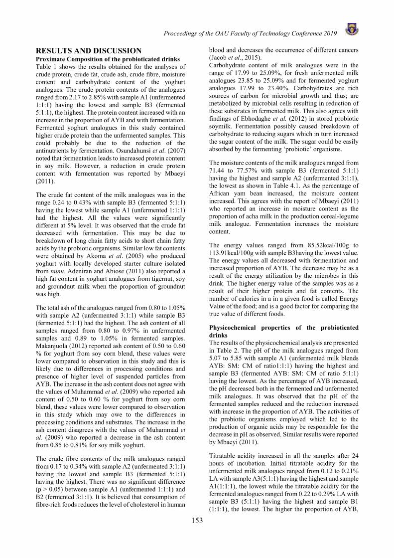
Proceedings of the OAU Faculty of Technology Conference 2019
153
RESULTS AND DISCUSSION Proximate Composition of the probioticated drinks Table 1 shows the results obtained for the analyses of crude protein, crude fat, crude ash, crude fibre, moisture content and carbohydrate content of the yoghurt analogues. The crude protein contents of the analogues ranged from 2.17 to 2.85% with sample A1 (unfermented 1:1:1) having the lowest and sample B3 (fermented 5:1:1), the highest. The protein content increased with an increase in the proportion of AYB and with fermentation. Fermented yoghurt analogues in this study contained higher crude protein than the unfermented samples. This could probably be due to the reduction of the antinutrients by fermentation. Osundahunsi et al. (2007) noted that fermentation leads to increased protein content in soy milk. However, a reduction in crude protein content with fermentation was reported by Mbaeyi (2011). The crude fat content of the milk analogues was in the range 0.24 to 0.43% with sample B3 (fermented 5:1:1) having the lowest while sample A1 (unfermented 1:1:1) had the highest. All the values were significantly different at 5% level. It was observed that the crude fat decreased with fermentation. This may be due to breakdown of long chain fatty acids to short chain fatty acids by the probiotic organisms. Similar low fat contents were obtained by Akoma et al. (2005) who produced yoghurt with locally developed starter culture isolated from nunu. Adeniran and Abiose (2011) also reported a high fat content in yoghurt analogues from tigernut, soy and groundnut milk when the proportion of groundnut was high. The total ash of the analogues ranged from 0.80 to 1.05% with sample A2 (unfermented 3:1:1) while sample B3 (fermented 5:1:1) had the highest. The ash content of all samples ranged from 0.80 to 0.97% in unfermented samples and 0.89 to 1.05% in fermented samples. Makanjuola (2012) reported ash content of 0.50 to 0.60 % for yoghurt from soy corn blend, these values were lower compared to observation in this study and this is likely due to differences in processing conditions and presence of higher level of suspended particles from AYB. The increase in the ash content does not agree with the values of Muhammad et al. (2009) who reported ash content of 0.50 to 0.60 % for yoghurt from soy corn blend, these values were lower compared to observation in this study which may owe to the differences in processing conditions and substrates. The increase in the ash content disagrees with the values of Muhammad et al. (2009) who reported a decrease in the ash content from 0.85 to 0.81% for soy milk yoghurt. The crude fibre contents of the milk analogues ranged from 0.17 to 0.34% with sample A2 (unfermented 3:1:1) having the lowest and sample B3 (fermented 5:1:1) having the highest. There was no significant difference (p > 0.05) between sample A1 (unfermented 1:1:1) and B2 (fermented 3:1:1). It is believed that consumption of fibre-rich foods reduces the level of cholesterol in human
blood and decreases the occurrence of different cancers (Jacob et al., 2015). Carbohydrate content of milk analogues were in the range of 17.99 to 25.09%, for fresh unfermented milk analogues 23.85 to 25.09% and for fermented yoghurt analogues 17.99 to 23.40%. Carbohydrates are rich sources of carbon for microbial growth and thus; are metabolized by microbial cells resulting in reduction of these substrates in fermented milk. This also agrees with findings of Ebhodaghe et al. (2012) in stored probiotic soymilk. Fermentation possibly caused breakdown of carbohydrate to reducing sugars which in turn increased the sugar content of the milk. The sugar could be easily absorbed by the fermenting ‘probiotic’ organisms. The moisture contents of the milk analogues ranged from 71.44 to 77.57% with sample B3 (fermented 5:1:1) having the highest and sample A2 (unfermented 3:1:1), the lowest as shown in Table 4.1. As the percentage of African yam bean increased, the moisture content increased. This agrees with the report of Mbaeyi (2011) who reported an increase in moisture content as the proportion of acha milk in the production cereal-legume milk analogue. Fermentation increases the moisture content. The energy values ranged from 85.52kcal/100g to 113.91kcal/100g with sample B3having the lowest value. The energy values all decreased with fermentation and increased proportion of AYB. The decrease may be as a result of the energy utilization by the microbes in this drink. The higher energy value of the samples was as a result of their higher protein and fat contents. The number of calories in a in a given food is called Energy Value of the food; and is a good factor for comparing the true value of different foods. Physicochemical properties of the probioticated drinks The results of the physicochemical analysis are presented in Table 2. The pH of the milk analogues ranged from 5.07 to 5.85 with sample A1 (unfermented milk blends AYB: SM: CM of ratio1:1:1) having the highest and sample B3 (fermented AYB: SM: CM of ratio 5:1:1) having the lowest. As the percentage of AYB increased, the pH decreased both in the fermented and unfermented milk analogues. It was observed that the pH of the fermented samples reduced and the reduction increased with increase in the proportion of AYB. The activities of the probiotic organisms employed which led to the production of organic acids may be responsible for the decrease in pH as observed. Similar results were reported by Mbaeyi (2011). Titratable acidity increased in all the samples after 24 hours of incubation. Initial titratable acidity for the unfermented milk analogues ranged from 0.12 to 0.21% LA with sample A3(5:1:1) having the highest and sample A1(1:1:1), the lowest while the titratable acidity for the fermented analogues ranged from 0.22 to 0.29% LA with sample B3 (5:1:1) having the highest and sample B1 (1:1:1), the lowest. The higher the proportion of AYB,
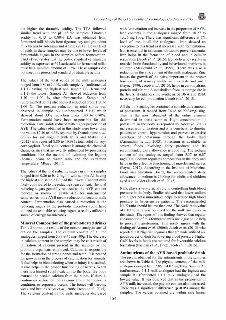
Proceedings of the OAU Faculty of Technology Conference 2019
154
the higher the titratable acidity. The TTA followed similar trend with the pH of the samples. Titratable acidity of 0.13 to 0.80% LA was obtained from fermented milk blends from tigernut, soy and groundnut milk blends by Adeniran and Abiose (2011). Lower level of acids in these samples may be due to lower levels of fermentable sugars in the samples before fermentation. FAO (1986) states that the codex standard of titratable acidity as expressed as % Lactic acid for fermented milks must be a minimal amount of 0.3%. These samples did not meet this prescribed standard of titratable acidity. The values of the total solids of the milk analogues ranged from 0.80 to 1.40% with sample A1 (unfermented 1:1:1) having the highest and sample B3 (fermented 5:1:1) the lowest. Sample A1 showed reduction from 1.40 to 1.00 % after fermentation. Sample A2 (unfermented 3:1:1) also showed reduction from 1.20 to 1.00 %. The greatest reduction in total solids was observed in sample A3 (unfermented 5:1:1) which showed about 33% reduction from 1.40 to 0.80%. Fermentation could have been responsible for this reduction. Total solids reduced with higher proportion of AYB. The values obtained in this study were lower than the values 12.40 to14.5% reported by Osundahunsi et al. (2007) for soy yoghurt with fruits and Makanjuola (2012) who reported 8.80 to 10.98% total solid for soy-corn yoghurt. Total solid content is among the chemical characteristics that are overtly influenced by processing conditions like the method of hydrating the legume (beans), beans to water ratio and the extraction temperature (Mbaeyi, 2011). The values of the total reducing sugars in all the samples ranged from 0.26 to 0.42 mg/ml with sample A1 having the highest and sample B3 had the lowest. Coconut milk likely contributed to the reducing sugar content. The total reducing sugars generally reduced as the AYB content reduced as shown in (Table 4.2) for unfermented samples. As more AYB meant reduction of coconut milk content. Fermentation also caused a reduction in the reducing sugars as the probiotic microbes could have utilized the available reducing sugars, a readily utilizable source of energy for microbes. Mineral Composition of the probioticated drinks Table 3 shows the results of the mineral analysis carried out on the samples. The calcium content of all the analogues ranged from 5.97-9.46 mg/100g. The decrease in calcium content in the samples may be as a result of utilization of calcium present in the samples by the probiotic organisms employed. Calcium is responsible for the formation of strong bones and teeth. It is needed for growth as in the process of calcification for animals. It also helps in blood clotting when an injury is sustained. It also helps in the proper functioning of nerves. When there is a limited supply calcium to the body, the body extracts the needed calcium from the bones. If there is continuous extraction of calcium from the bones, a condition, osteoporosis occurs. The bones will become weak and brittle (Aliyu et al., 2008; Jacob et al., 2015). The calcium content of the milk analogues decreased
with fermentation and increase in the proportion of AYB. Iron contents in the analogues ranged from 10.27 to 13.26 mg/100g. There was significant difference at 5% level of iron in all the analogues. Iron showed an exception to this trend as it increased with fermentation. Iron is essential in in human nutrition to prevent anaemia. Iron helps in the formation of blood and in cellular respiration (Jacob et al., 2015). Iron deficiency results in retarded brain functionality and behavioural problems in children (McDonald et al., 1995). There was also a reduction in the zinc content of the milk analogues. Zinc boosts the growth of the hairs, important in the proper functioning of sensory ability such as taste and smell (Payne, 1990; Jacob et al., 2015), helps in carbohydrate, protein and vitamin A metabolism from its storage site in the livers. It enhances the synthesis of DNA and RNA necessary for cell production (Jacob et al., 2015). All the milk analogues contained a considerable amount of potassium. It ranged from 74.48 to 90.34mg/100g. This is the most abundant of the entire element determined in these samples. High concentration of potassium in the body as reported by Adeyeye (2002) increases iron utilization and it is beneficial to diuretic patients to control hypertension and prevent excessive excretion of potassium through the body fluid (Arinanthan et al., 2003). Potassium is available in several foods involving dairy products and its recommended daily allowance is 3500 mg. The sodium content of the analogues ranged from 5.37 to 6.87 mg/100g. Sodium regulates homeostasis in the body and helps in the effective functioning of muscles and nerves (Payne, 2012). According to the Institute of Medicine, Food and Nutrition Board, the recommended daily allowance for sodium is 2400mg for adults and children aged 4 and older (Jacob et al., 2012). Na/K plays a very crucial role in controlling high blood pressure in the body. Studies showed that lower sodium and higher potassium intake helps to reduce high blood pressure in hypertensive patients. The recommended Na/K ratio should be less than one. The Na/K ratio value of 0.07 to 0.08 was obtained for the milk analogues in this study. The report of this finding showed that regular consumption of this fermented milk analogue could help to prevent hypertension. This result agrees with the finding of Aremu et al. (2006); Jacob et al. (2015) who reported that Nigerian legumes that are underutilised are good sources of diets for lowering blood pressure. Higher Ca/K levels in foods are required for favourable calcium formation (Nieman et al., 1992; Jacob et al., 2015).
Antinutrients of the AYB-based probiotic drink The results obtained for the antinutrients in the samples are shown in Table 4. The phytate contents of the milk analogues ranged from 2.85 to 4.07 mg/100g. Sample A3 (unfermented 5:1:1 milk analogue) had the highest and sample B1 (fermented 1:1:1 milk analogue) had the lowest value. It was observed that as the proportion of AYB milk increased, the phytate content also increased. There was a significant difference (p<0.05) among the samples. The values obtained are within safe limits.
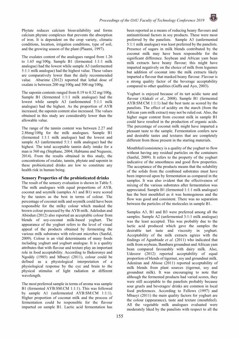
Proceedings of the OAU Faculty of Technology Conference 2019
155
Phytate reduces calcium bioavailability and forms calcium phytate complexes that prevents the absorption of iron. It is dependent on the crop variety, climatic conditions, location, irrigation conditions, type of soil, and the growing season of the plant (Plaami, 1997). The oxalates content of the analogues ranged from 1.26 to 1.65 mg/100g. Sample B1 (fermented 1:1:1 milk analogue) had the lowest while sample A3 (unfermented 5:1:1 milk analogue) had the highest value. These values are comparatively lower than the daily recommended value. Aburime (2012) reported that lethal dose of oxalate is between 200 mg/100g and 500 mg/100g. The saponin contents ranged from 0.19 to 0.32 mg/100g. Sample B1 (fermented 1:1:1 milk analogue) had the lowest while sample A3 (unfermented 5:1:1 milk analogue) had the highest. As the proportion of AYB increased, the saponin content also increased. The values obtained in this study are considerably lower than the allowable value. The range of the tannin content was between 2.27 and 2.86mg/100g for the milk analogues. Sample B1 (fermented 1:1:1 milk analogue) had the lowest and sample A3 (unfermented 5:1:1 milk analogue) had the highest. The total acceptable tannin daily intake for a man is 560 mg (Stephane, 2004; Habtamu and Negussie, 2014). From the results obtained in this study, the concentrations of oxalate, tannin, phytate and saponin in these probioticated drinks are low to constitute any health risk in human being.
Sensory Properties of the probioticated drinks The result of the sensory evaluation is shown in Table 5. The milk analogues with equal proportions of AYB, coconut and soymilk (samples A1 and B1) were scored by the tasters as the best in terms of colour. The percentage of coconut milk and soymilk could have been responsible for the milky colour which masked the brown colour possessed by the AYB milk. Adelodun and Abiodun (2012) also reported an acceptable colour from blends of soy-coconut milk-based yoghurt. The appearance of the yoghurt refers to the level of visual appeal of the products obtained by fermenting the various milk substrates with relevant microbes (Sanful, 2009). Colour is an vital determinanta of many foods including yoghurt and yoghurt analogue. It is a quality attributes that with flavour and texture play an important role in food acceptability. According to Ihekoronye and Ngoddy (1985) and Mbaeyi (2011), colour could be defined as a physiological interpretation of a physiological response by the eye and brain to the physical stimulus of light radiation at different wavelength. The most preferred sample in terms of aroma was sample B1 (fermented AYB:SM:CM 1:1:1). This was followed by sample A1 (unfermented AYB:SM:CM 1:1:1). Higher proportion of coconut milk and the process of fermentation could be responsible for the flavour imparted on sample B1. Lactic acid fermentation has
been reported as a means of reducing beany flavours and antinutritional factors in soy products. These were most preferred by the panelists. Sample A3 (unfermented 5:1:1 milk analogue) was least preferred by the panelists. Presence of sugars in milk blends contributed by the coconut milk may have been responsible for the significant difference. Soybean and African yam bean milk extracts have beany flavour; this might have imparted negatively on the choice of milk from legumes but addition of coconut into the milk extracts likely imparted a flavour that masked beany flavour. Flavour is a strong quality factor of the beverage acceptability compared to other qualities (Gaffa and Ayo, 2003). Yoghurt is enjoyed because of its tart acidic taste and flavour (Alakali et al., 2008). Sample B1 (fermented AYB:SM:CM 1:1:1) had the best taste as scored by the panelists. The effect of acidity on the starch (from the African yam milk extract) may not be ruled out. Also, the higher sugar content from coconut milk in sample B1 could have resulted in the production of organic acids. The percentage of coconut milk might have imparted a pleasant taste to the sample. Fermentation confers new and desirable tastes and textures that are completely different from those present in the starting materials. Mouthfeel/consistency is a quality of the yoghurt to flow without having any residual particles on the containers (Sanful, 2009). It refers to the property of the yoghurt indicative of the smoothness and good flow properties. The acceptance of the products means that the solubility of the solids from the combined substrates must have been improved upon by fermentation as compared in the samples. It was also evident that the effectiveness of mixing of the various substrates after fermentation was appreciated. Sample B1 (fermented 1:1:1 milk analogue) has the best mouthfeel as it was homogenous and the flow was good and consistent. There was no separation between the particles of the molecules in sample B1. Samples A3, B1 and B3 were preferred among all the samples. Sample A2 (unfermented 3:1:1 milk analogue) was the least accepted. This was probably due to the lactic acid produced which gave the samples the desirable tart taste and viscosity in yoghurt. Acceptability of the milk extracts agrees with the findings of Agunbiade et al. (2011) who indicated that milk from soybean, Bambara groundnut and African yam bean compared favourably with dairy milk. Also, Udeozor (2012) reported acceptability of equal proportion of blends of tigernut, soy and groundnut milk. Adeniran and Abiose (2011) reported acceptability of milk blends from plant sources (tigernut, soy and groundnut milk). It was encouraging to note that although the fermented products had varied scores, they were still acceptable to the panelists probably because sour gruels and beverages/ drinks are common in local food preferences. According to Fellows (1997) and Mbaeyi (2011) the main quality factors for yoghurt are the colour (appearance), taste and texture (mouthfeel). All the vegetable milk analogues evaluated were moderately liked by the panelists with respect to all the
Proceedings of the OAU Faculty of Technology Conference 2019
156
attributes for yoghurt. The sourness of the yoghurt expresses the level of astringency produced by lactic acid by the action of Lactobacillus delbrueckii on lactose in the substrate (Sanful, 2009; Mbaeyi, 2011). Also, the aroma produced from the fermentation of the yoghurt is particularly due to acetaldehyde formation and other volatile aromatic compounds resulting from the anaerobic breakdown of carbohydrates by these beneficial microbes (Sanful, 2009; Mbaeyi, 2011). CONCLUSIONS The study produced probioticated drinks from various blends of milk analogues from AYB, soybean and coconut. The study concluded that increase in the proportion of AYB produced analogues of high acidity, low pH, high protein, high potassium, energy and acceptable sensory qualities. Sample with equal ratio was the most acceptable of all samples. ACKNOWLEDGMENT The authors are grateful to the Department of Food Science and Technology for the assistance rendered during the study.
REFERENCES Adelodun, L. K. and Abiodun, O. O., Effect of different
concentrations of coconut milk on the chemical and sensory properties of soy-coconut milk-based yoghurt. Food and Public Health, 2(4): 85-91, 2012.
Adeniran, H. A. and Abiose, S. H., Characterization and hydrolytic activities of amylases from Bacillus licheniformis and Aspergillus niger cultivated on agricultural residues. African Journal of Biotechnology, 11(6): 1465-1477, 2011.
Adeniran, H. A., Olaniyi, O. A. and Abiose, S. H., Viability and effect of probiotic lactic acid bacteria isolated from locally fermented foods in a non-dairy beverage from African yam bean. Proceedings of the OAU Faculty of Technology Conference, 71-78, 2015.
Adeyeye, E. I., Determination of chemical composition of the nutritionally valuable parts of male and female common West African fresh water crab (Sudananoutes africanus). Food Chemistry, 28-30, 2002.
Agunbiade, S. O., Amosu, A. M., Mand, D. A. and Omeonu, P. E., The physicochemical and organoleptic properties of milk fabricated from Glycine max, Vigna subterranean and Sphenostylis stenocarpa. Journal of Chemical and Pharmaceutical Research, 3(6): 918-924, 2011.
Akoma, O., Musa, S., Akoma, A. O. and Asunmo, R. G., Nutritional values of yoghurt produced with locally developed starter culture isolated from nono. Proceedings of the 29th NIFST AGM/Conference, Ebonyi State University, Abakaliki, 11th-13th October, 5: 292-293, 2005.
Alakali, J. S., Okonkwo, T. M and Iordye, E. M., Effect of stabilizers on the physico-chemical and sensory attributes of thermized yoghurt. African Journal of Biotechnology, 7(2): 158-163, 2008.
Aliyu, A. B., Musa, A. M. and Oshaniyi, J. A., Phytochemical analysis and mineral composition analysis of some medicinal plants of Northern Nigeria. Nigerian Journal of Pharmaceutical Sciences, 7(1): 119-121, 2008.
Amakoromo, E. R., Innocent-Adiele, H. C. and Njoku, H. O., Physicochemical quality of a yoghurt-like product from African yam bean. Report Opinion, 4(4): 58-61, 2012.
Aminigo, E. R., Lehtola, P. S. and Metzger, L. E., Nutritive composition and physical characteristics of supplemented imitation milk from African yam bean (Sphenostylis stenocarpa). Global Journal of Pure and Applied Sciences, 13: 457-462, 2007.
Arinanthan, V., Mohan, V. R. and Britto, A. J., Chemical composition of certain tribal pulses in South India. International Journal of Food Sciences and Nutrition, 3: 103-107, 2003.
Association of Official Analytical Chemists (AOAC). Official Methods of Analysis. Washington, DC: Association of Official Analytical Chemists, 2000.
Brunner, J. H., Direct spectrophometric determination of saponin. Annal of Chemistry, 42: 1752-1754, 1984.
Ebhodaghe, S. O., Abiose, S. H. and Adeniran, H. A., Assessment of physico-chemical characteristics, viability and inhibitory effect of Bifidobacteria in soymilk. Journal of Food Research, 1(2): 159-169, 2012.
FAO., Composition Analytical Methods. In: Manuals of Food Quality Control. Food and Agricultural Organization of the United Nations, Rome, Pp 204-230, 1986.
Fellows, P., Traditional Foods Processing for Profit. 1st edition, Intermediate Technology Publisher Limited, London, 1997.
Folasade, M. and Oyenike, O., Effect of sesame seed addition on the chemical and sensory qualities of sorghum based kunun-zaki drink. African Journal of Food Science and Technology, 3(9): 204-212, 2012.
Gaffa, T. and Ayo, J. A., Physiochemical and sensory effects of Cadaba farinosa crude extract on cereal starches during kunun-zaki production. Pakistan Journal of Nutrition, 2(1): 13-17, 2013.
Habtamu, F. G. and Negussie, R., Antinutritional factors in plant foods: potential health benefits and adverse effects. Global Advanced Research Journal of Food Science and Technology, 3(4): 103-117, 2014.
Hassan, A. M., Abdallah, M. I. M, Bazalou, M. S. and Abo-Samra, R. G., Effect of probiotics bacteria isolated from yoghurts produced in Damietta city on some pathogenic bacteria. Proceedings of the 6th Animal Wealth Research Conference in the Middle East and North Africa Hurghada information center- 27-30, 01–14, September, 2013.
Ihekoronye, A. I. and Ngoddy, P. O., Integrated Food Science and Technology for Tropics, London, UK, Pp 1-386, 1985.
Jacob, A. G., Etong, D. I. and Tijani, A., Proximate, mineral and anti-nutritional factors in tigernut, soyabean and coconut milk sources. International
Proceedings of the OAU Faculty of Technology Conference 2019
157
Journal of Agriculture and Biology, 9(5), 785 -787, 2005.
Larmond, E., Laboratory methods for sensory evaluation of foods. Canadian Agricultural publications. Series IV, Ottawa. Canada, 1991.
Lukas, C. S. and Makarkas, P., Phytic acid and other phosphorus compounds of bean (Phaseolus vulgaris). Journal of Agricultural Education and Chemistry, 23: 13-15, 1975.
Makanjuola, O. M., Production and quality evaluation of soy-corn yoghurt. Advanced Journal of Food Science and Technology, 4(3): 130-134, 2012.
Makkar, H. P., Blummel, M. and Becken, K., Determination of tannin and its correlation with chemical and protein precipitation method. Journal of Science, food and Agriculture, 6: 161-165, 1993.
Mbaeyi, I. E., Studies on cereal-legume blend potential for development of novel non-dairy probiotic yoghurt analogues. Ph. D submitted to the Department of Microbiology, University of Nigeria, Nsukka, 2011.
McDonald, A., Edwards, R. A., Greenhulgh, F. D. and Morgan, C. A., Animal Nutrition. Prentices Hall, London, Pp 101-122, 1995.
Muhammad, B. F., Abubakar, M. M. and Adegbola, T. A., Effect of period and condition of storage on properties of yoghurt produced from cow milk and soymilk materials. Research Journal of Dairy Science, 2: 18 – 24, 2009.
Nieman, D. C., Butterworth, D. E and Nieman, C. N., Nutrition watch, WMC Brown Publishers, Dubugye, USA, 1992.
Oke, O. L., The role of hydrocyanide acid in nutrition. World review of Nutrition and Dietetics, 11: 118-147, 1969b.
Osundahunsi, O. F., Amosu, D., Ifesan, B. O. T., Quality evaluation and acceptability of soy-yoghurt with different colours and fruit flavours. American Journal of Food Technology, 2: 273-280, 2007.
Payne, W. J. A. An Introduction to Animal Husbandry in the Tropics. Longman Publishers, Singapore, 92- 110, 1990.
Plaami, S., Myoinositol phosphates: Analysis, content in foods and effects in nutrition. British Microbiology Research Journal, 3(2): 198-205, 1997.
Sanful, R. E., The use of tigernut (Cyperus esculentus), cow milk and their composite as substrates for yoghurt production. Pakistan Journal of Nutrition, 8(6): 755-758, 2009.
Soccol, C. R., Vandernberghe, L. P., Spier, M. R., Medeiros, A. B. P, Yamaguishi, C. T, Lindner, J. D, Pandey, A. and Thomaz-Soccol, V., The potential of probiotics. Food Technology and Biotechnology, 48(4): 413-434, 2010.
Stéphane, R., Interaction of grape seed procyanidins with various proteins in relation to wine fining. Journal of Science Food Agriculture, 57: 111-125, 2004.
Udeozor, L. O., Tigernut-soy milk drink: preparation, proximate composition and sensory qualities. International Journal of Food and Nutrition Science, 1(4): 18-26, 2012.
Yilmaz-Ersan, L and Kurdal, E., The production of set-type-bio-yoghurt with commercial probiotic culture. International Journal of Chemical Engineering and Applications, 5(5): 402-408, 2014.

Proceedings of the OAU Faculty of Technology Conference 2019
158
Figure 2: Flow Chart for the production of fermentd milk analogues Table 1: Proximate Composition of the Milk Analogues (%)
Means with the same
superscript within
columns are not
significantly different at P < 0.05
A1 unfermented
(1:1:1)
AYB:SM:CM B1 fermented(1:1:1) AYB:SM:CM A2 unfermented (3:1:1) AYB:SM:CM B2 fermented(3:1:1) AYB:SM:CM A3 unfermented (5:1:1) AYB:SM:CM B3 fermented(5:1:1) AYB:SM:CM
Samples Protein Fat Ash Fibre Moisture Carbohydrate Energy (kcal/100g)
A1 2.17±0.01d 0.43±0.00
a 0.97±0.00
a 0.21±0.00
b 72.37±0.03
b 23.85±0.01
a 107.95b
A2 2.27±0.03c 0.23±0.00
c 0.80±0.00
b 0.17±0.00
c 71.44±0.00
b 25.09±0.03
a 113.91a
A3 2.45±0.01b 0.34±0.00
b 0.88±0.00
b 0.23±0.00
b 72.57±0.02
b 23.53±0.04
a 106.98b
B1 2.38±0.07b 0.25±0.00
c 0.89±0.00
b 0.21±0.00
b 72.87±0.02
b 23.40±0.01
a 105.37b
B2 2.51±0.03b 0.28±0.00
c 0.98±0.00
a 0.21±0.00
b 74.47±0.03
b 21.55±0.05
b 98.76c
B3 2.85±0.07a 0.24±0.00
c 1.05±0.00
a 0.34±0.00
a 77.53±0.02
a 17.99±0.04
c 85.52d

Proceedings of the OAU Faculty of Technology Conference 2019
159
Table 2: Physicochemical Properties of the Milk Analogues Samples pH TTA (%LA) Total Solids (%) Total Reducing Sugars(mg/ml)
A1 5.85±0.02
a
0.12±0.01c
1.40±0.28a
0.42±0.03a
A2 5.66±0.01
b
0.18±0.01b
1.20±0.57a
0.34±0.07b
A3 5.36±0.01
c
0.21±0.01b
1.40±0.28a
0.28±0.03c
B1 5.29±0.00
c
0.22±0.01b
1.00±0.28b
0.39±0.17a
B2 5.10±0.01
d
0.28±0.03a
1.00±0.28b
0.26±0.00c
B3 5.07±0.02
d
0.29±0.06a
0.80±0.00b
0.27±0.00c
Means with the same superscript within columns are not significantly different at P < 0.05 A1 unfermented (1:1:1) AYB:SM:CM B1 fermented(1:1:1) AYB:SM:CM A2 unfermented (3:1:1) AYB:SM:CM B2 fermented(3:1:1) AYB:SM:CM A3 unfermented (5:1:1) AYB:SM:CM B3 fermented(5:1:1) AYB:SM:CM
Table 3: Mineral Contents of the Milk Analogues (mg/100g)
Samples Ca Fe Zn K Na Na/K ratio
A1 9.64±0.02a 10.26±0.00
c 5.59±0.00
b 88.84±0.03
a 6.67±0.01
a 0.07
A2 8.85±0.00b 11.17±0.03
bc 6.36±0.01
a 90.34±0.01
a 6.87±0.01
a 0.08
A3 7.47±0.01c 12.36±0.01
b 5.48±0.01
b 85.27±0.03
b 5.97±0.00
b 0.07
B1 8.37±0.02b 10.69±0.00
c 4.87±0.01
c 80.13±0.00
c 6.77±0.00
a 0.08
B2 6.12±0.00d 12.45±0.01
b 6.67±0.00
a 77.77±0.03
c 5.37±0.02
b 0.07
B3 5.97±0.00d 13.26±0.00
a 4.74±0.01
c 74.48±0.02
c 5.45±0.01
b 0.07
Means with the same superscript within columns are not significantly different at P < 0.05 A1 unfermented (1:1:1) AYB:SM:CM B1 fermented(1:1:1) AYB:SM:CM A2 unfermented (3:1:1) AYB:SM:CM B2 fermented(3:1:1) AYB:SM:CM A3 unfermented (5:1:1) AYB:SM:CM B3 fermented(5:1:1) AYB:SM:CM
Table 4: Antinutrients of the Milk Analogues (mg/100g) Samples Phytate Tannin Saponin Oxalates A1 3.67±0.00b 2.65±0.01b 0.24±0.01b 1.43±0.01b
A2 3.76±0.01b 2.76±0.00a 0.28±0.00a 1.64±0.01a
A3 4.07±0.03a 2.86±0.03a 0.32±0.01a 1.65±0.02a
B1 2.85±0.01d 2.27±0.03c 0.19±0.00c 1.26±0.00c
B2 3.36±0.01bc 2.49±0.00bc 0.25±0.00b 1.29±0.00c
B3 3.59±0.00b 2.56±0.01b 0.25±0.00b 1.39±0.00b
Means with the same superscript within columns are not significantly different at P < 0.05 A1 unfermented (1:1:1) AYB:SM:CM B1 fermented(1:1:1) AYB:SM:CM A2 unfermented (3:1:1) AYB:SM:CM B2 fermented(3:1:1) AYB:SM:CM A3 unfermented (5:1:1) AYB:SM:CM B3 fermented(5:1:1) AYB:SM:CM
Table 5: Sensory Evaluation of the Milk Analogues Produced from Blends of AYB, Soybean and Coconut Samples Colour Mouthfeel Taste Flavour Overall acceptability A1 2.5±0.53a 1.2±0.03d 2.1±0.74b 2.4±0.27a 1.8±0.33b
A2 2.2±0.29b 2.2±0.25c 1.5±0.85c 1.4±0.84c 1.4±0.84c
A3 2.2±0.25b 2.6±0.23b 2.4±0.22b 2.1±0.74b 2.4±0.70a
B1 2.5±0.53a 3.0±0.93a 4.3±1.98a 2.5±0.53a 2.4±0.22a
B2 1.7±0.53c 1.9±0.52cd 1.7±0.30c 2.2±0.25b 2.0±0.21ab
B3 1.0±0.00d 2.3±0.67c 2.3±0.67b 1.6±0.22c 2.2±0.70a
Means with the same superscript within columns are not significantly different at P < 0.05 A1 unfermented (1:1:1) AYB:SM:CM B1 fermented(1:1:1) AYB:SM:CM A2 unfermented (3:1:1) AYB:SM:CM B2 fermented(3:1:1) AYB:SM:CM A3 unfermented (5:1:1) AYB:SM:CM B3 fermented(5:1:1) AYB:SM:CM
Proceedings of the OAU Faculty of Technology Conference 2019
160
DEGRADATION OF ASCORBIC ACID IN ORANGE JUICE FORTIFIED WITH LOW MOLECULAR WEIGHT PEPTIDES OBTAINED FROM PEPSIN
HYDROLYZED AMARANTH LEAF PROTEIN
A. A. Famuwagun*1, S. O. Gbadamosi1, K. A Taiwo1, R.E. Aluko2, D. J. Oyedele3 and O. C. Adebooye4
1Department of Food Science and Technology, Obafemi Awolowo University, Ile-Ife, Nigeria 2Department of Food and Human Nutritional Sciences,
University of Manitoba, Winnipeg, MB, Canada R3T 2N2 3 Departments of Soil Science and Land Management
Resources, Obafemi Awolowo University, Ile-Ife, Nigeria 4Department of Agronomy, Obafemi Awolowo University, Ile-Ife, Nigeria
*E-mail of Corresponding Author: [email protected]
ABSTRACT
Ascorbic acid is an essential nutrient required for good health. This study investigated the kinetics of degradation of ascorbic acid in freshly prepared orange juice samples containing <1kDa peptides obtained from pepsin-hydrolysed amaranth leaf protein. The <1 kDa peptides were separated from a pepsin hydrolysate of amaranth leaf protein through membrane ultrafiltration. The peptides were then incorporated into freshly prepared orange juice. The juice samples were stored at 4 ± 2 oC or 28 ± 2 oC for two months. The ascorbic acid contents of the stored orange juices were evaluated and their degradation kinetics monitored using Arrhenius equations. The results showed that rate of degradations of ascorbic acid in the juice samples was best fitted in first order kinetics. Juice samples stored at 28 ± 2 oC had higher rate constant and lower activation energies when compared with juice samples stored at 4 ± 2 oC. Also, juice samples without peptides had higher rate constant and lower activation energy, resulting in higher degradation of ascorbic acid when compared to juice sample that contained peptides. The study concluded that the presence of <1 kDa peptides retarded ascorbic acid degradation in the stored juice and storage temperature plays a role in the process.
Keywords: Arrhenius equation, functional ingredient, rate constants, leafy vegetables, peptides
INTRODUCTION Orange juice is one of the most popular fruit juices worldwide, probably due to its nutritional content, appealing color, refreshing sweet taste and presence of biologically active compounds, such as vitamin C (Wibowo et al., 2015). Vitamin C or ascorbic acid is a water-soluble vitamin and is very essential in maintaining the health of human beings, due to its reducing ability and oxygen scavenging effects (Udding et al., 2002). Vitamin C is very sensitive and can be destroyed when exposed to adverse conditions during fruit juice storage (Lee and Kader, 2000). Ascorbic acid can be oxidized reversibly to dehydroascorbic acid (DHAA), without losing its functionality. This is because the biological activity of ascorbic acid and DHAA are similar (Udding et al., 2002). Further degradation of DHAA to 2,3-diketogulonic acid (DKGA) leads to loss of biological activity. The ascorbic acid content of orange juice is about 140.08 ± 1.87 mg/100 mL (Famuwagun, 2019) and several factors that affect this value have been identified to include light exposure, level of dissolved oxygen, presence of metal ions, presence of sugar, level of additives and storage temperature (Udding
et al., 2002; Polydera et al., 2003; Burdurlu et al., 2006; Serpen, 2007). This degradation of vitamin C in orange juice, just like other fruit juices, is the main problem of the nutritional quality loss and has great implications on shelf life of the juice. This is because, vitamin C is usually considered as the nutrient quality indicator during processing and storage of juice, since it is generally observed that, if ascorbic acid is well retained, the other nutrients are mostly going to be retained (Franke et al., 2004). The functional drink sector is one of the thriving food sectors in the developed world, due to its immense contributions to the reduction of chronic diseases (Dominguez-Perles et al., 2011). Functional drinks are specialized forms of drinks that contain functional ingredients (natural or synthetic, which have been found to possess bioactive properties) that improves the performance of the drink beyond the conventional nutritional quality. Such ingredients may be added or present naturally in the drink (Dominguez-Perles et al.
Proceedings of the OAU Faculty of Technology Conference 2019
161
2011). Such drinks may be designed to target the reduction of some chronic diseases in the body. Food proteins are made up of several specific peptide sequences that remain inactive as long as they remain bonded to other amino acids
within the primary structure (Aluko, 2015). Treatment of proteins with an enzyme or a combination of enzymes can lead to proteolysis that
releases these peptide sequences. The free forms of peptides can be used against human degenerative diseases such as hypertension and anti-diabetic (Aluko, 2015). Such peptides could be encapsulated as nutraceuticals or as functional ingredients. Such ingredients requiring a transport medium requires that such fortification does not interfere with bioactive properties of vitamin C. Also, juice fortification should not speed up the degradation vitamin C. To study the extent potential benefits of peptide fortification, kinetic order and rate constants of the vitamin C degradation over a stored period of time need to be investigated. This is because kinetic order and rate constant are the basic requirements to define shelf-life of fruit juices. The kinetic models can be used for economic assessments of food quality (Valdramidis et al. 2010), and in predicting the influence of several experimental variables on critical nutritional values. This work was designed to investigate the kinetics of ascorbic acid degradation in peptide-fortified orange juice stored at ambient and refrigerated storage conditions. This is necessary to better understand the interaction of the functional ingredient with orange juice components and also to provide information on the potential of the juice as a potential vehicle for isolated peptide. MATERIALS AND METHODS Preparation of <1 kDa Leaf Protein-Derived Peptides The leaves of amaranth were dried and subjected to acetone extraction (1:10 w/v) on a magnetic stirrer for 2 h and the mixture filtered using a muslin cloth to obtain the partially de-greened leaf powder. A protein isolate was produced from the partially degreened powder by combined processes of solubilization, precipitation, neutralization and lyophilization. The protein isolate was subsequently hydrolyzed using pepsin (a food grade enzyme) to obtain the protein hydrolysate as described by Omoni and Aluko (2006) with little modification. The hydrolysate was further separated by passing through an ultrafiltration stirred cell Amicon-8400 (Millipore Corp., Billerica, MA, USA) using a 1 kDa molecular cut-off weight (MWCO) membrane, and the permeate lyophilized to obtain the peptide powder. Preparation of Orange Juice Matured and ripe sweet oranges (Citrus sinensis), three days after harvest were purchased from the
Teaching and Research Farms, Obafemi Awolowo University, Ile-Ife, Nigeria. The fruits were sorted and defect-free oranges were considered for the juice extraction. Extraction of juice from orange fruits was carried out following the method described by Akusu et al. (2016). The selected fruits were sorted and washed thoroughly under running tap water. The pericarps were removed with the aid of stainless-steel knife and the juice was extracted using a hand-held juice extractor to obtain a clear orange juice. Preparation of Peptide-Fortified Orange Juice and Storage Studies The fresh orange juice produced was distributed equally into 162 different sterilized polyethylene bottles and 0.1 % sodium benzoate added and homogenized. The <1 kDa peptide was incorporated into each container at the levels where the peptide could scavenge 50 % free radicals (EC 50) and inhibited alpha amylase and glucosidase enzymes (EC50), (Famuwagun, 2019) and the mixture was homogenized. The peptide incorporated juice samples and the control juice (juice without peptide) were capped and pasteurized at 80 ºC for 10 minutes. The juice samples were cooled under running water and stored at ambient (28 ± 2 oC) or refrigerated (4 ± 2 oC) conditions for two months. Estimation of Ascorbic Acid Content of Stored Juice Samples Ascorbic acid content in the samples was estimated by titrimetric method as described by Rekha et al. (2012). Five millilitres of standard ascorbic acid (100 μg/mL) were measured into a conical flask containing 10 mL 4% oxalic acid. The mixture was titrated against the 0.0005M of 2,6-dichlorophenol indophenols dye (DCPIP). The appearance and persistence of pink colour for 30 seconds is taken as the end point. The amount of dye consumed (V1 mL) is equivalent to the amount of ascorbic acid. Five millilitres of sample (prepared by taking 5 mL of juice in 100 mL 4% oxalic acid) was measured inside a conical flask containing 10 mL 4% oxalic acid in a conical flask and titrated against the dye (V2 mL). The amount of ascorbic acid was calculated using the formula;
𝐴𝑠𝑐𝑜𝑟𝑏𝑖𝑐 𝑎𝑐𝑖𝑑 (𝑚𝑔/𝑚𝐿) =𝑋𝑖 𝑚𝑔
𝑉𝑖 𝑥
𝑉 𝑖𝑖
15 𝑚𝑙 𝑥
100 𝑚𝐿
𝑚𝐿 𝑜𝑓 𝑠𝑎𝑚𝑝𝑙𝑒 𝑢𝑠𝑒𝑑 𝑓𝑜𝑟 𝑎𝑛𝑎𝑙𝑦𝑠𝑖𝑠 (1)
𝑋𝑖 (𝑚𝑔) =𝑞𝑢𝑎𝑛𝑡𝑖𝑡𝑦 𝑜𝑓 𝑎𝑠𝑐𝑜𝑟𝑏𝑖𝑐 𝑎𝑐𝑖𝑑 𝑑𝑖𝑠𝑠𝑜𝑙𝑣𝑒𝑑 𝑖𝑛 𝑎 𝑘𝑛𝑜𝑤𝑛 𝑣𝑜𝑙𝑢𝑚𝑒 𝑜𝑓 𝑜𝑥𝑎𝑙𝑖𝑐 𝑎𝑐𝑖𝑑 𝑉𝑖 = 𝑣𝑜𝑙𝑢𝑚𝑒 𝑜𝑓 𝑑𝑦𝑒 𝑐𝑜𝑛𝑠𝑢𝑚𝑒𝑑 𝑏𝑦 𝑡ℎ𝑒 𝑠𝑡𝑎𝑛𝑑𝑎𝑟𝑑 𝑉𝑖𝑖 = 𝑣𝑜𝑙𝑢𝑚𝑒 𝑜𝑓 𝑑𝑦𝑒 𝑐𝑜𝑛𝑠𝑢𝑚𝑒𝑑 𝑏𝑦 𝑡ℎ𝑒 𝑠𝑎𝑚𝑝𝑙𝑒 15 𝑚𝐿= 𝑡𝑜𝑡𝑎𝑙 𝑣𝑜𝑙𝑢𝑚𝑒 𝑜𝑓 𝑠𝑎𝑚𝑝𝑙𝑒 𝑎𝑛𝑑 𝑜𝑥𝑎𝑙𝑖𝑐 𝑡𝑖𝑡𝑟𝑎𝑡𝑒𝑑
100 𝑚𝐿 =𝑣𝑜𝑙𝑢𝑚𝑒 𝑜𝑓 𝑜𝑥𝑎𝑙𝑖𝑐 𝑎𝑐𝑖𝑑 𝑠𝑜𝑙𝑢𝑡𝑖𝑜𝑛 𝑢𝑠𝑒𝑑 𝑖𝑛 𝑑𝑖𝑠𝑠𝑜𝑙𝑣𝑖𝑛𝑔 𝑡ℎ𝑒 𝑠𝑎𝑚𝑝𝑙𝑒
Degradation Kinetics of Ascorbic Acid in the Juice Samples The degradation kinetics model of the ascorbic acid of the juice samples during storage of was studied using
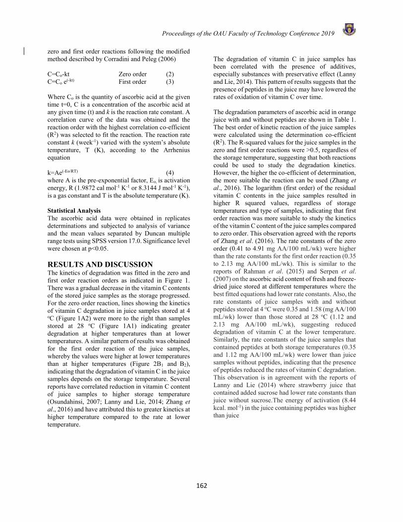
Proceedings of the OAU Faculty of Technology Conference 2019
162
zero and first order reactions following the modified method described by Corradini and Peleg (2006) C=Co-kt Zero order (2) C=Co e(-kt) First order (3) Where Co is the quantity of ascorbic acid at the given time t=0, C is a concentration of the ascorbic acid at any given time (t) and k is the reaction rate constant. A correlation curve of the data was obtained and the reaction order with the highest correlation co-efficient (R2) was selected to fit the reaction. The reaction rate constant k (week-1) varied with the system’s absolute temperature, T (K), according to the Arrhenius equation k=Ae(-Eo/RT) (4) where A is the pre-exponential factor, Eo, is activation energy, R (1.9872 cal mol-1 K-1 or 8.3144 J mol-1 K-1), is a gas constant and T is the absolute temperature (K). Statistical Analysis The ascorbic acid data were obtained in replicates determinations and subjected to analysis of variance and the mean values separated by Duncan multiple range tests using SPSS version 17.0. Significance level were chosen at p<0.05. RESULTS AND DISCUSSION The kinetics of degradation was fitted in the zero and first order reaction orders as indicated in Figure 1. There was a gradual decrease in the vitamin C contents of the stored juice samples as the storage progressed. For the zero order reaction, lines showing the kinetics of vitamin C degradation in juice samples stored at 4 oC (Figure 1A2) were more to the right than samples stored at 28 oC (Figure 1A1) indicating greater degradation at higher temperatures than at lower temperatures. A similar pattern of results was obtained for the first order reaction of the juice samples, whereby the values were higher at lower temperatures than at higher temperatures (Figure 2B1 and B2), indicating that the degradation of vitamin C in the juice samples depends on the storage temperature. Several reports have correlated reduction in vitamin C content of juice samples to higher storage temperature (Osundahinsi, 2007; Lanny and Lie, 2014; Zhang et al., 2016) and have attributed this to greater kinetics at higher temperature compared to the rate at lower temperature.
The degradation of vitamin C in juice samples has been correlated with the presence of additives, especially substances with preservative effect (Lanny and Lie, 2014). This pattern of results suggests that the presence of peptides in the juice may have lowered the rates of oxidation of vitamin C over time. The degradation parameters of ascorbic acid in orange juice with and without peptides are shown in Table 1. The best order of kinetic reaction of the juice samples were calculated using the determination co-efficient (R2). The R-squared values for the juice samples in the zero and first order reactions were >0.5, regardless of the storage temperature, suggesting that both reactions could be used to study the degradation kinetics. However, the higher the co-efficient of determination, the more suitable the reaction can be used (Zhang et al., 2016). The logarithm (first order) of the residual vitamin C contents in the juice samples resulted in higher R squared values, regardless of storage temperatures and type of samples, indicating that first order reaction was more suitable to study the kinetics of the vitamin C content of the juice samples compared to zero order. This observation agreed with the reports of Zhang et al. (2016). The rate constants of the zero order (0.41 to 4.91 mg AA/100 mL/wk) were higher than the rate constants for the first order reaction (0.35 to 2.13 mg AA/100 mL/wk). This is similar to the reports of Rahman et al. (2015) and Serpen et al. (2007) on the ascorbic acid content of fresh and freeze-dried juice stored at different temperatures where the best fitted equations had lower rate constants. Also, the rate constants of juice samples with and without peptides stored at 4 oC were 0.35 and 1.58 (mg AA/100 mL/wk) lower than those stored at 28 oC (1.12 and 2.13 mg AA/100 mL/wk), suggesting reduced degradation of vitamin C at the lower temperature. Similarly, the rate constants of the juice samples that contained peptides at both storage temperatures (0.35 and 1.12 mg AA/100 mL/wk) were lower than juice samples without peptides, indicating that the presence of peptides reduced the rates of vitamin C degradation. This observation is in agreement with the reports of Lanny and Lie (2014) where strawberry juice that contained added sucrose had lower rate constants than juice without sucrose.The energy of activation (8.44 kcal. mol-1) in the juice containing peptides was higher than juice
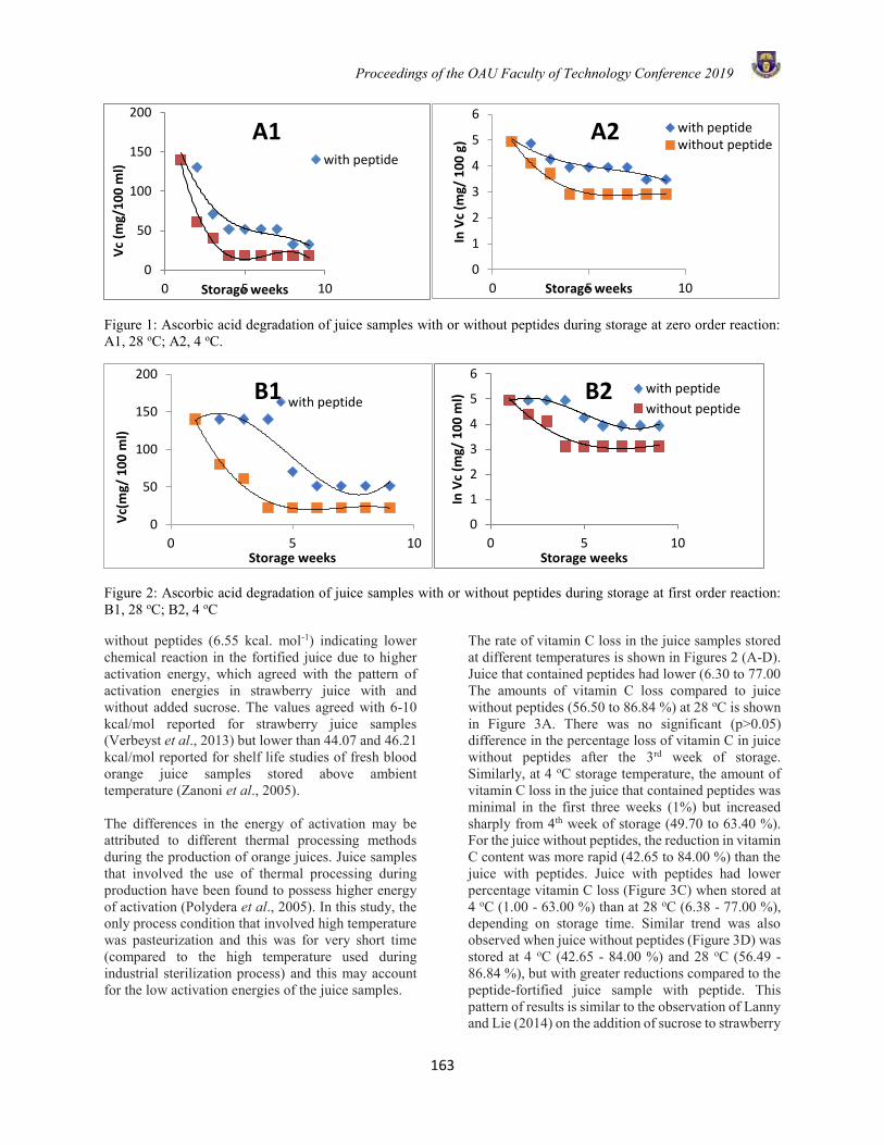
Proceedings of the OAU Faculty of Technology Conference 2019
163
Figure 1: Ascorbic acid degradation of juice samples with or without peptides during storage at zero order reaction: A1, 28 oC; A2, 4 oC.
Figure 2: Ascorbic acid degradation of juice samples with or without peptides during storage at first order reaction: B1, 28 oC; B2, 4 oC
without peptides (6.55 kcal. mol-1) indicating lower chemical reaction in the fortified juice due to higher activation energy, which agreed with the pattern of activation energies in strawberry juice with and without added sucrose. The values agreed with 6-10 kcal/mol reported for strawberry juice samples (Verbeyst et al., 2013) but lower than 44.07 and 46.21 kcal/mol reported for shelf life studies of fresh blood orange juice samples stored above ambient temperature (Zanoni et al., 2005). The differences in the energy of activation may be attributed to different thermal processing methods during the production of orange juices. Juice samples that involved the use of thermal processing during production have been found to possess higher energy of activation (Polydera et al., 2005). In this study, the only process condition that involved high temperature was pasteurization and this was for very short time (compared to the high temperature used during industrial sterilization process) and this may account for the low activation energies of the juice samples.
The rate of vitamin C loss in the juice samples stored at different temperatures is shown in Figures 2 (A-D). Juice that contained peptides had lower (6.30 to 77.00 The amounts of vitamin C loss compared to juice without peptides (56.50 to 86.84 %) at 28 oC is shown in Figure 3A. There was no significant (p>0.05) difference in the percentage loss of vitamin C in juice without peptides after the 3rd week of storage. Similarly, at 4 oC storage temperature, the amount of vitamin C loss in the juice that contained peptides was minimal in the first three weeks (1%) but increased sharply from 4th week of storage (49.70 to 63.40 %). For the juice without peptides, the reduction in vitamin C content was more rapid (42.65 to 84.00 %) than the juice with peptides. Juice with peptides had lower percentage vitamin C loss (Figure 3C) when stored at 4 oC (1.00 - 63.00 %) than at 28 oC (6.38 - 77.00 %), depending on storage time. Similar trend was also observed when juice without peptides (Figure 3D) was stored at 4 oC (42.65 - 84.00 %) and 28 oC (56.49 - 86.84 %), but with greater reductions compared to the peptide-fortified juice sample with peptide. This pattern of results is similar to the observation of Lanny and Lie (2014) on the addition of sucrose to strawberry
0
50
100
150
200
0 5 10
Vc
(mg/
10
0 m
l)
Storage weeks
A1with peptide
0
1
2
3
4
5
6
0 5 10
In V
c (m
g/ 1
00
g)
Storage weeks
A2 with peptidewithout peptide
0
50
100
150
200
0 5 10
Vc(
mg/
10
0 m
l)
Storage weeks
B1with peptide
0
1
2
3
4
5
6
0 5 10
In V
c (m
g/ 1
00
ml)
Storage weeks
B2 with peptide
without peptide
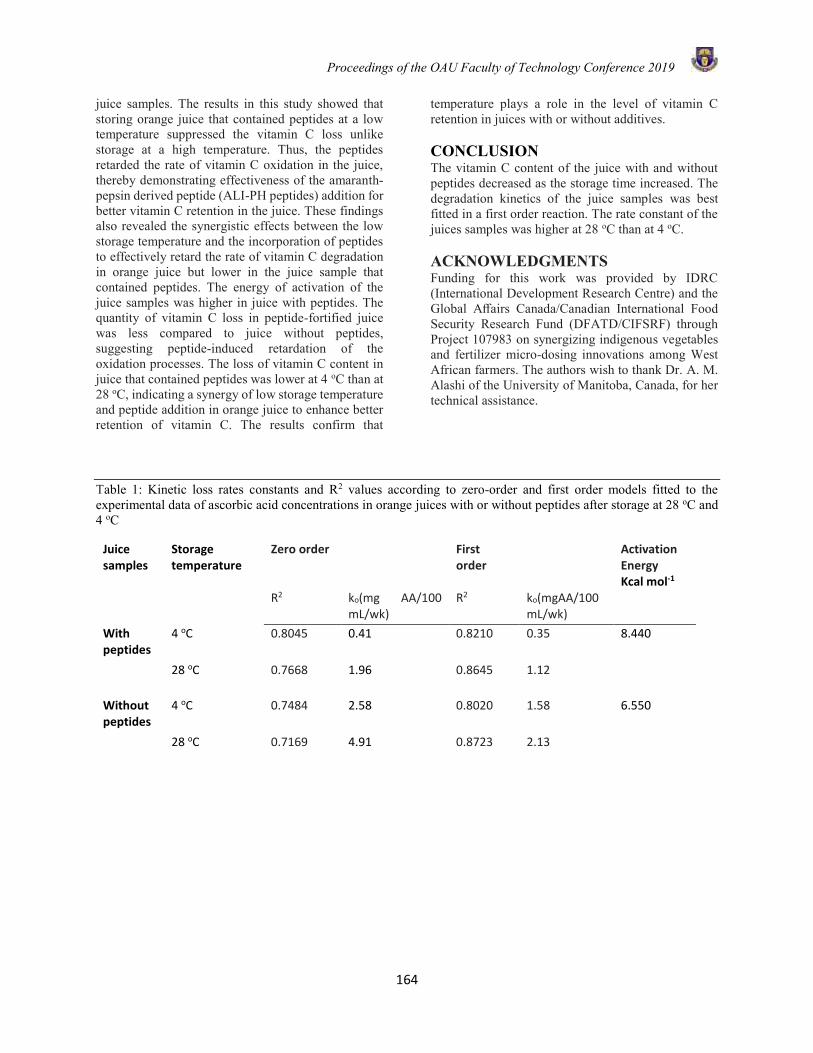
Proceedings of the OAU Faculty of Technology Conference 2019
164
juice samples. The results in this study showed that storing orange juice that contained peptides at a low temperature suppressed the vitamin C loss unlike storage at a high temperature. Thus, the peptides retarded the rate of vitamin C oxidation in the juice, thereby demonstrating effectiveness of the amaranth-pepsin derived peptide (ALI-PH peptides) addition for better vitamin C retention in the juice. These findings also revealed the synergistic effects between the low storage temperature and the incorporation of peptides to effectively retard the rate of vitamin C degradation in orange juice but lower in the juice sample that contained peptides. The energy of activation of the juice samples was higher in juice with peptides. The quantity of vitamin C loss in peptide-fortified juice was less compared to juice without peptides, suggesting peptide-induced retardation of the oxidation processes. The loss of vitamin C content in juice that contained peptides was lower at 4 oC than at 28 oC, indicating a synergy of low storage temperature and peptide addition in orange juice to enhance better retention of vitamin C. The results confirm that
temperature plays a role in the level of vitamin C retention in juices with or without additives. CONCLUSION The vitamin C content of the juice with and without peptides decreased as the storage time increased. The degradation kinetics of the juice samples was best fitted in a first order reaction. The rate constant of the juices samples was higher at 28 oC than at 4 oC. ACKNOWLEDGMENTS Funding for this work was provided by IDRC (International Development Research Centre) and the Global Affairs Canada/Canadian International Food Security Research Fund (DFATD/CIFSRF) through Project 107983 on synergizing indigenous vegetables and fertilizer micro-dosing innovations among West African farmers. The authors wish to thank Dr. A. M. Alashi of the University of Manitoba, Canada, for her technical assistance.
Table 1: Kinetic loss rates constants and R2 values according to zero-order and first order models fitted to the experimental data of ascorbic acid concentrations in orange juices with or without peptides after storage at 28 oC and 4 oC
Juice samples
Storage temperature
Zero order First order
Activation Energy Kcal mol-1
R2 ko(mg AA/100 mL/wk)
R2 ko(mgAA/100 mL/wk)
With peptides
4 oC 0.8045 0.41 0.8210 0.35 8.440
28 oC 0.7668 1.96 0.8645 1.12
Without peptides
4 oC 0.7484 2.58 0.8020 1.58 6.550
28 oC 0.7169 4.91 0.8723 2.13
Proceedings of the OAU Faculty of Technology Conference 2019
165
A
1 2 3 4 5 6 7 80
20
40
60
80
100
with peptide without peptide
a a a a a abb
bcccc
d e
f
Storage time (weeks)
Loss
of V
itami
n C (%
)
B
1 2 3 4 5 6 7 80
20
40
60
80
100
a a a aaa
bb bbbc
cc
dd d
Storage time (weeks)
Loss
of V
itami
n C (%
)
1 2 3 4 5 6 7 80
20
40
60
80
100
Ambient Refrigerated
C
a ab bbbbbbb
c c
d ee e
Storage time (weeks)
Loss
of V
itami
n C (%
)
1 2 3 4 5 6 7 80
20
40
60
80
100D
a a a a a aa a a a a a
bc c
d
Storage time (weeks)Lo
ss of
Vita
min C
(%)
Figure 3: Comparison of Loss of Vitamin C in (A) Juice samples at 28 oC (B) Juice samples at 4oC (C) Storage of Juice with Peptides (D) Storage of Juice without peptides
REFERENCES Akusu, O. M., Kiin-Kabari, D. B., Ebere, C. O.,
Quality Characteristics of Orange/Pineapple Fruit Juice Blends. American Journal of Food Science and Technology, 4(2): 43-47 DOI: 10.12691/ajfst-4-2-3, 2016.
Aluko, R. E., Anti-hypertensive peptides from food proteins. Annual Review in Food Science and Technology, 6: 235–262, 2015.
Burdurlu, H. S., Koca, N., Karadeniz, F., Degradation of Vitamin C in Citrus Juice Concentrates during Storage. Journal of Food Engineering 74: 211-216, 2006.
Corradini, M.G., Peleg, M., Prediction of vitamins loss during non-isothermal heat processes and storage with non-linear kinetic models. Trends in Food Science and Technology, 17(1): 24-34, 2006.
Dominguez-Perles, R., Moreno, D. A., Carvajal, M. and Garcia-Viguera, C., Composition and antioxidant capacity of a novel beverage produced with green tea and minimally-processed by products of broccoli. Innovative Food Science and Emerging Technology, 12: 361–368, 2011.
Famuwagun A. A., Functional and bioactive properties of protein isolates and hydrolysates of amaranth, eggplant and fluted
pumpkin leafy vegetables and application as functional ingredient. Unpublished Ph.D. Research Thesis at the Department of Food Science and Technology, Obafemi Awolowo University, Ile-Ife, Nigeria, 2019.
Franke, A. A., Custer, L. J., Arakaki, C., Murphy, S. P., Vitamin C and flavonoid Levels of fruits and vegetables consumed in Hawaii. Journal of Food Composition and Analysis, 17: 1-35, 2004.
Lanny, S., Lie, H., Study on the kinetics of vitamin c degradation in fresh strawberry. Procedia Chemistry, 9: 62 – 68, 2014.Lee, S.K., Kader, A.A., Preharvest and
postharvest factors influencing vitamin C content of horticultural crops. Postharvest Biology and Technology, 20(3): 207-220, 2000.
Omoni, A., Aluko, R.E., Mechanism of the inhibition of calmodulin-dependent neuronal-nitric oxide synthase by flaxseed protein hydrolysates. Journal of America Oil Chemistry, 83: 335–340, 2006.
Polydera, A.C., Stoforos, N. G., Taoukis, P. S., Comparative shelf life study and vitamin C loss kinetics in pasteurised and high pressure processed reconstituted orange juice. Journal of Food Engineering, 60: 21-29, 2003.

Proceedings of the OAU Faculty of Technology Conference 2019
166
Polydera, A.C., Stoforos, N.G., Taoukis, P.S., Quality degradation kinetics of pasteurised and high pressure processed fresh Navel orange juice: Nutritional parameters and shelf life. Innovative Food Science and Emerging Technology, 6(1): 1-9, 2005.
Zanoni, B., Pagliarini, E. Galli A., Laureati, M., Shelf-life prediction of fresh blood orange juice. Journal of Food Engineering, 70(4): 512-517, 2005.
Zhang, J., Han, H., Xia, J., Gao, M., Degradation Kinetics of Vitamin C in Orange and Orange Juice during Storage. Journal of Food Engineering, 23:1-12, 2016.
Rahman, M.S., Al-Rizeiqi, N., Guizani, M.S., AlRuzaiqi, A.H. Al-Aamri, Zainab, S. Stability of vitamin C in fresh and freeze-dried capsicum stored at different temperatures. Journal of Food Science and Technology, 52(3): 1691-1697, 2015.
Rekha, C., Poornim, G., Manasa, M., Abhipsa, V., Devi, J., Kumar,H. and Kekuda, T., Ascorbic acid, total phenol content and antioxidant activity of fresh juices of four ripe and unripe citrus fruits. Chemical Science and Transport, 1(2): 303–310, 2012.
Serpen, A. and Gökmen, V., Reversible degradation kinetics of ascorbic acid under reducing and oxidizing conditions. Food Chemistry, 104: 721–725, 2007.
Udding, M. S., Hawlader, M.N.A., Luo, D., Mujumdar, A. S., Degradation of ascorbic acid in dried guava during storage. Journal of Food Engineering, 51: 21-26, 2002.
Valdramidis, V. P., Cullen, P. J., Tiwari, B. K., O’Donnell, C. P., Quantitative modelling approaches for ascorbic acid degradation and non-enzymatic browning of orange juice during ultrasound processing. Journal of Food Engineering, 96: 449-454, 2010.
Verbeyst, L., Bogaerts, R., Van der, P. I., Hendrickx, M., van Loey, A., Modelling of vitamin C degradation during thermal and high pressure treatments of red fruit. Food and Bioprocess Technology, 6: 1015-1023, 2013.
Wibowo, S. T., Grauwet, J.S., Santiago, J., Tomic, L., Vervoort, M., H. and Loey, A.V., Quality changes of pasteurised orange juice during storage: A kinetic study of specific parameters and their relation to colour instability. Food Chemistry, 187: 140-151, 2015
Proceedings of the OAU Faculty of Technology Conference 2019
167
DESIGN MODIFICATIONS AND PERFORMANCE EVALUATION OF A CENTRIFUGAL IMPACT PALM NUTS CRACKER
T. A. Morakinyo*1 Department of Food Science and Technology, Faculty of Technology,
Obafemi Awolowo University, Ile-Ife, Nigeria.
* Email of Corresponding Author: [email protected]
ABSTRACT This study presented a modified centrifugal impact palm nuts cracker for traditional and small-scale palm oil processors. The physical properties of Dura and Tenera cultivars palm nuts were investigated prior to machine design. The modified prototype was developed and evaluated using palm nuts of three categories of geometrical mean diameters (GMD) at steady drying temperature of 80 oC and drying periods of 15, 18 and 21 hrs. The results of the physical properties such as length, breadth, thickness, mass, GMD and sphericity were in the range 25.19-35.84 (mm), 18.69-26.44 (mm), 15.05-21.71 (mm), 4.60-11.57 (g), 19.10-27.58 (mm) and 0.75-0.77 (%); 26.90-33.97 (mm), 17.89-24.57 (mm), 14.32-20.44 (mm), 3.28-8.84 (g), 18.50-25.84 (mm) and 0.71-0.75 (%) for Dura and Tenera palm nuts cultivars, respectively. The optimum throughput at 15, 18 and 21 hrs drying periods were: 200 and 180, 240 and 218, 235 and 230 (kg/hr) for Dura and Tenera cultivars, respectively. The optimum cracking efficiency of 88% was obtained across all level of GMD, while the predicted value above this threshold was 94% for Dura cultivar only. The damaged percentage and recovery efficiency have threshold of 8% and 6% for both Dura and Tenera cultivars, respectively. Hence, the determination of physical properties prior to development of this machine and increase in speed, modified cracking drum and impact rotor enhanced its performance. Keywords: Modified centrifugal impact palm nut cracker, cracking efficiency, geometric mean diameter, and optimization. INTRODUCTION The oil palm is a perennial tree crop that originated from West Africa but is now cultivated in plantations across tropical Africa, Southeast Asia and Southern America more than its origin (Mutsaers, 2019). It is botanically known as Elaeis guineensis. The major varieties are Dura, Tenera and Pisifera (Adzimah and Seckley, 2009), but the commercial and most prominent cultivars are Dura and Tenera (Morakinyo and Bamgboye, 2015). The primary products of palm tree are palm fruits, palm wine, broom and timber. However, the secondary products are palm oil, palm nut; palm kernel and shells likewise palm kernel oil and cake. A palm fruit is made of a smooth outer skin (exocarp), a fibrous pulp (mesocarp) which contains palm oil, a centrally placed palm nut with hard shell (endocarp) and the kernel in which palm kernel oil is derived. Palm kernel oil is useful in making soap, biodiesel, glycerin, margarine, candle, pomade, oil paint and polish. The shells are used as biomass to fuel boiler and brake pad composite for automobile, while palm kernel meals or cakes are utilized to produce animal feeds (Gbadamosi, 2006; Adebayo, 2004; Emeka and Olomu, 2007). Palm kernel oil processing mills are not common as oil palm fruit processing mills in Nigeria, due to inadequate technological advancement in this sector. However, exportation of palm nut and kernel into Europe and North
Asia countries from Nigeria and Indonesia is highly prolific (FAO, 2002). Recently, there is an industrial revolution that necessitated for increase in the demand of palm kernel and shell in the Southwestern Nigeria. This necessitated for promulgation of government policy by placing embargo on importation of palm kernel oil. The industrialization of this section has become desirable coupled with astronomical increase in the selling price of palm kernel oil. In order to meet up with high demand of this product, there is an urgent need to modify indigenous palm nut crackers for optimum cracking efficiency and durability. Previously, some researchers reported on the development of various palm nut crackers of different cracking mechanism such as centrifugal impact, hammer or rod impact and roller crackers (Adejugbe et al., 2017; Kayo, 2006). Antia et al. 2014, investigated the optimum moisture content value and drying period that enhanced palm nut cracker efficiency. They reported that the optimum moisture content value and drying period were 2.5% (dry basis) and 18 hrs, respectively for both Dura and Tenera palm nuts cultivars at maximum cracking efficiency of 84%. However, for industrialization, critical modifications and optimization are still necessary in order to achieve higher efficiencies, durability and reliability. Hence this study.
Proceedings of the OAU Faculty of Technology Conference 2019
168
MATERIALS AND METHODS Materials The materials for this study were Dura and Tenera palm nuts. The Dura cultivar palm nuts were obtained from oil palm mill at Eleweeran, Ede Road, Ile-Ife, Osun state, Nigeria with initial moisture content of about 23.5% (wet basis) while Tenera cultivar palm nuts of initial moisture content of about 22.8% were obtained from oil palm mill at Elere Adubi, Itori, Ogun State, Nigeria. The palm nuts of each cultivar were sorted and graded into three categories of axial dimensions: small, medium and large sizes. From the population of individual sizes were selected 100 pieces of palm nuts randomly to form eighteen samples in triplicates to be dried in three distinctive periods of 15, 18 and 21 hrs. Each category of small, medium and large sizes was kept inside labeled black polyethylene bag to determine physical properties using standard procedures according to their respective cultivar (Morakinyo and Bamgboye, 2015). The corresponding axial dimensions such as: length, breadth and thickness, geometric mean diameter, sphericity of each cultivar were measured using digital caliper while their corresponding mass was determined using electronic digital weighing balance, model: Scout Pro SPU 401 with standard error of 0.001 mm. The average values of the geometrical mean diameters of both cultivars were calculated to categorize their sizes (18.80 mm, 22.46 mm and 26.72 mm) to reduce the experimental runs. The data obtained were used as machine design parameters for the prototype modifications. All materials of construction were procured from Owode Onirin, Iron market, Ikorodu, Lagos. The exiting force convection biomass-fired cabinet drier of three tray compartments was used for the drying of eighteen samples at steady temperature of 80 oC to the almost equal value of moisture content at retention periods of 15, 18 and 21 hrs for Dura and Tenera cultivars consecutively. The drying operation was carried out for each drying period sequentially by loading 100 pieces of each sample of the geometrical mean diameter category in three replicate inside tray. However, for each drying period, six experimental runs were observed concurrently which summed up to eighteen experimental runs. The dried samples were kept inside desiccators for cooling and then cracked using modified centrifugal impact palm nuts cracker. The machine characteristics evaluated were throughput, the cracking efficiency, damaged percentage and the recovery efficiency for optimum purpose. METHOD Mechanical Properties The breaking force along longitudinal and axial directions of palm nut previously reported by Davies (2012) was adopted as 2.83 and 11.00 kN, respectively.
Machine Design Considerations The following factors were considered while designing the new prototype. The average geometrical mean diameter of the two palm nuts cultivars was used to determine the clearance between the beater and the cracking ring. However to eliminate high rate of abrasion of the cracking ring, high carbon steel material was hardened and tempered to the hardness value of 65 HRC. To achieve optimum impact force for effective cracking, high speed electric motor of 2850 rpm with the propelling impact of 3 ph was adopted. Four beaters impeller type was designed to ensure adequate and uniform cracking of the nuts. The beaters were arranged at quadrant pattern in equal inter-distance to each other. The driven shaft and bearing housings were machined using appropriate fits and tolerances. Balancing of impeller was achieved by grinding and re-weighing the individual beater as centrifugal arm on a digital weighing scale until equal weight was achieved to eliminate throwing force. After welding, the impeller was re-calibrated on the lathe machine for accuracy. Machine Design Calculations for the Modified Centrifugal Palm Nuts Cracker The cracking ring design Consider a palm nut under a centrifugal force creating impact force against the inner diameter of a circular cracking ring at a constant velocity. Let M= mass of the palm nut in kg, r = radius of the circular cracking ring in mm, v= constant angular velocity of the palm nut. The Equations 1-3 were adopted as reported by Khurmi (2005)
Centrifugal acceleration of a body = a = v2
r ( m
sec2) (1)
The centrifugal force, Pe= m ×v2
r = mɷ2 r (N) (2)
However, ω= 2πN
60 (3)
Since in the design considerations, one of the critical factors is speed The impeller speed selected was 2850
2 rpm = 1425 rpm,
Hence ω = 149.3 rad
sec .
For the inner radius of the cracking ring of 130 mm and with Dura palm nut mass of 0.01157 kg, The centrifugal force = 0.01157 × 149.32 × 130 = 33.521 kN. For Tenera of 8.84 g = 0.00884 kg, the centrifugal force = 25.62 kN. These centrifugal forces calculated from above were generated from the proposed speed of the electric motor and average mass of Dura and Tenera palm nuts cultivars. These were found to be higher than the longitudinal and axial breaking forces of palm nut previously reported by Davies (2012) reported as 2.83 and 11.00 kN, respectively; hence the design calculated values were adequate for
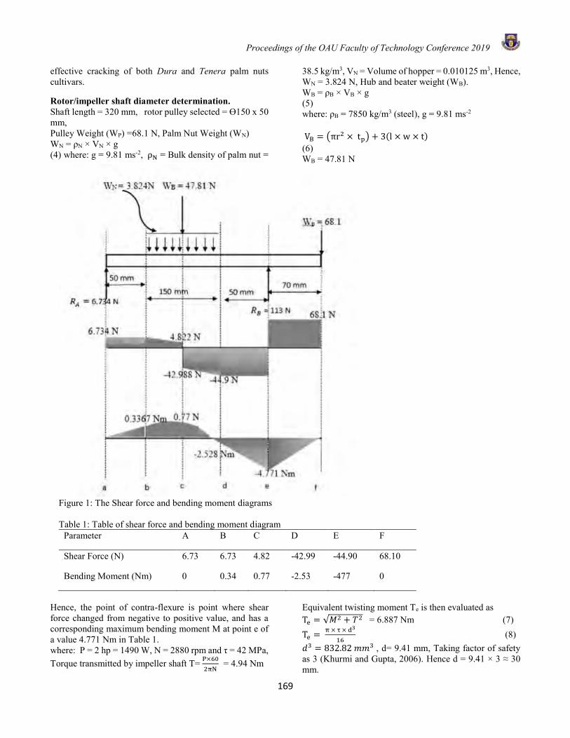
Proceedings of the OAU Faculty of Technology Conference 2019
169
effective cracking of both Dura and Tenera palm nuts cultivars. Rotor/impeller shaft diameter determination. Shaft length = 320 mm, rotor pulley selected = Ө150 x 50 mm, Pulley Weight (WP) =68.1 N, Palm Nut Weight (WN) WN = ρN × VN × g (4) where: g = 9.81 ms-2, ρN = Bulk density of palm nut =
38.5 kg/m3, VN = Volume of hopper = 0.010125 m3, Hence, WN = 3.824 N, Hub and beater weight (WB). WB = ρB × VB × g (5) where: ρB = 7850 kg/m3 (steel), g = 9.81 ms-2
VB = (πr2 × tp) + 3(l × w × t) (6) WB = 47.81 N
Figure 1: The Shear force and bending moment diagrams Table 1: Table of shear force and bending moment diagram
Parameter A B C D E F
Shear Force (N) 6.73 6.73 4.82 -42.99 -44.90 68.10
Bending Moment (Nm) 0 0.34 0.77 -2.53 -477 0
Hence, the point of contra-flexure is point where shear force changed from negative to positive value, and has a corresponding maximum bending moment M at point e of a value 4.771 Nm in Table 1. where: P = 2 hp = 1490 W, N = 2880 rpm and τ = 42 MPa, Torque transmitted by impeller shaft T=
P×60
2πN = 4.94 Nm
Equivalent twisting moment Te is then evaluated as Te = √𝑀2 + 𝑇2 = 6.887 Nm (7) Te =
π × τ × d3
16 (8)
𝑑3 = 832.82 𝑚𝑚3 , d= 9.41 mm, Taking factor of safety as 3 (Khurmi and Gupta, 2006). Hence d = 9.41 × 3 ≈ 30 mm.
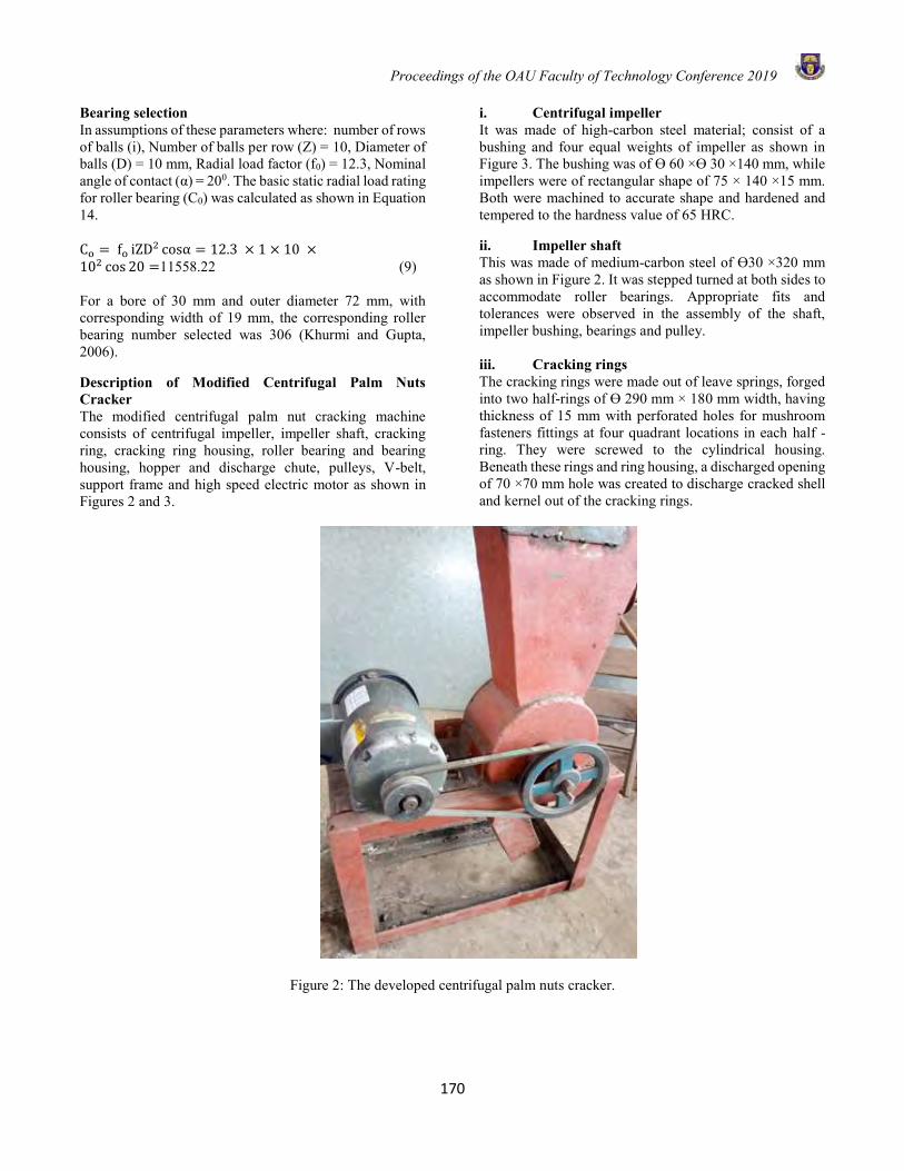
Proceedings of the OAU Faculty of Technology Conference 2019
170
Bearing selection In assumptions of these parameters where: number of rows of balls (i), Number of balls per row (Z) = 10, Diameter of balls (D) = 10 mm, Radial load factor (f0) = 12.3, Nominal angle of contact (α) = 200. The basic static radial load rating for roller bearing (C0) was calculated as shown in Equation 14. Co = fo iZD2 cosα = 12.3 × 1 × 10 ×102 cos 20 =11558.22 (9) For a bore of 30 mm and outer diameter 72 mm, with corresponding width of 19 mm, the corresponding roller bearing number selected was 306 (Khurmi and Gupta, 2006). Description of Modified Centrifugal Palm Nuts Cracker The modified centrifugal palm nut cracking machine consists of centrifugal impeller, impeller shaft, cracking ring, cracking ring housing, roller bearing and bearing housing, hopper and discharge chute, pulleys, V-belt, support frame and high speed electric motor as shown in Figures 2 and 3.
i. Centrifugal impeller It was made of high-carbon steel material; consist of a bushing and four equal weights of impeller as shown in Figure 3. The bushing was of Ɵ 60 ×Ɵ 30 ×140 mm, while impellers were of rectangular shape of 75 × 140 ×15 mm. Both were machined to accurate shape and hardened and tempered to the hardness value of 65 HRC. ii. Impeller shaft This was made of medium-carbon steel of Ɵ30 ×320 mm as shown in Figure 2. It was stepped turned at both sides to accommodate roller bearings. Appropriate fits and tolerances were observed in the assembly of the shaft, impeller bushing, bearings and pulley. iii. Cracking rings The cracking rings were made out of leave springs, forged into two half-rings of Ɵ 290 mm × 180 mm width, having thickness of 15 mm with perforated holes for mushroom fasteners fittings at four quadrant locations in each half -ring. They were screwed to the cylindrical housing. Beneath these rings and ring housing, a discharged opening of 70 ×70 mm hole was created to discharge cracked shell and kernel out of the cracking rings.
Figure 2: The developed centrifugal palm nuts cracker.

Proceedings of the OAU Faculty of Technology Conference 2019
171
Figure 3: Exploded view of the modified centrifugal palm nuts cracker.
iv. Cracking rings housing This was made of low-carbon steel material of a cylindrical shape as shown in Figure 2. It has diameter of 300 mm, width of 150 mm and thickness of 5 mm. There are two outer cover plates made of low-carbon steel of Ɵ 300 × 5 mm thickness with a center hole which accommodate impeller shaft. At the upper part, 150 × 150 mm hole was made to position hopper. v. Hopper The hopper was made of low-carbon steel material of 2.5 mm thickness of a trapezoidal shape; through which the materials were fed into the cracking unit. It has dimensions of 300 × 150 × 150 (mm) equivalent to a volume of 0.010125 m3 using Equation 10. 𝑉ℎ =
1
2(𝑎 + 𝑏) × ℎ × 𝑙 (10)
vi. The frame This was made of angle iron of 60×60×4 (mm) having a vertical height, breadth and length of 410 × 270× 620 (mm), for the positioning of cracking ring housing, bearings and electric motor. Performance Evaluation of the Machine The throughput of the machine was evaluated by weighing 100 pieces of palm nuts and feeding them into the machine through the hopper. The cracker was operated at a constant speed of 2850 rpm, as one of the modifications factor in this prototype, higher than the speed of electric motor previously reported ( Koya, 2006, ; Antia et al., 2014). The cracking period was recorded for each cracking operation. This
procedure was replicated for each sample from three trays for the corresponding size and cultivar. The average machine throughput (Mt) was calculated using Equation 11. Mt =
Weight (kg)
Time Taken (hr) (11)
Cracking efficiency The cracking efficiency is the ratio of the number of cracked nuts to the total number of nuts fed into the cracker expressed in percentage. This was determined using the mathematical expression reported by Gbabo et al. (2013) depicted as Equation (12). CEFF =
NC
NT × 100 (12)
where, CEFF is the Cracking efficiency (%), NC = the number of the cracked NT is the initial total number of the nuts Damaged percentage The damaged percentage is the ratio of the number of broken nuts to the total number of nuts fed into the cracker expressed in percentage. This was determined using the expression reported by Gbabo et al. (2013) depicted as Equation 13. DDP =
NB
NT × 100 (13)
where, DDP is the damaged percentage (%), NB = the number of the broken nuts NT is the initial total number of the nuts

Proceedings of the OAU Faculty of Technology Conference 2019
172
Recovery efficiency The recovery efficiency is the ratio of the un-cracked nuts to the total number of the nuts before cracking. This is expressed in percentage as reported by Gbabo et al. (2013). This was determined using Equation (14). REFF =
NUB
NT × 100 (14)
where, REFF is the recovery efficiency (%), NUN = the number of unbroken shelled nuts NT is the total number of nuts Data Analysis The experimental data of the physical properties were analyzed using descriptive and inferential statistics to
determine means and standard deviation. However, experimental design for the performance characterizations of the modified centrifugal palm nut cracker was generated using Response Surface Method with Multilevel-Categoric Factors of Design-Expert 11.1.0 (Stat-Ease, Inc., 2019). Table 1 showed the 3 Categoric factors of 2×3×3 factorial design as cultivar, geometrical mean diameter (size) and drying period, respectively. Eighteen experimental runs were generated and corresponding four responses (cracking efficiency, throughput, and damage percentage and recovery efficiency) were obtained during each run. The optimum performance characterizations of this machine were established.
Table 2: The Multilevel-Categoric factors for the modified centrifugal palm nut cracker characterization
Categoric factors Unit Type Levels Level 1 Level 2 Level 3
Cultivar Nominal 2 Dura Tenera
Geometrical Mean Diameter Mm Nominal 3 18.80 22.46 26.72
Drying Period Hrs Nominal 3 15.00 18.00 21.00
Table 3: Results of the physical properties of Dura cultivar palm nuts at 23.5% (wet bases) moisture content. Palm nuts size
Length (mm) Breadth (mm) Thickness (mm)
Mass
(g)
Geometric Mean Diameter (mm)
Sphericity (%)
Small 25.19±4.30 18.69±2.07 15.05±1.75 4.60±0.75 19.10±1.32 0.75±0.05
Medium 30.24±4.47 22.44±2.26 17.36±2.03 7.08±1.14 23.05±1.40 0.82±0.03
Large 35.84±4.80 26.44±2.53 21.71±2.27 11.57±2.09 27.58±3.30 0.77±0.02
Table 4: Results of the physical properties of Tenera cultivar palm nuts at 22.8% (wet bases) moisture content Palm nuts size
Length (mm) Breadth (mm) Thickness (mm)
Mass
(g)
Geometric Mean Diameter (mm)
Sphericity (%)
Small 26.90±4.21 17.89±1.90 14.32±1.62 3.28±0.62 18.50±2.86 0.71±0.02
Medium 28.34±4.21 20.90±2.10 16.53±1.52 5.35±0.68 21.86±3.06 0.72±0.06
Large 33.97±5.23 24.57±2.72 20.44±1.93 8.84±1.59 25.84±3.15 0.75±0.07
RESULTS AND DISCUSSIONS Physical properties of the palm nuts Tables 3 -4, showed the results of the physical properties of palm nuts such as length, breadth, thickness, mass,
geometrical mean diameter and sphericity ranges of both palm nuts cultivars at their respective initial moisture contents.
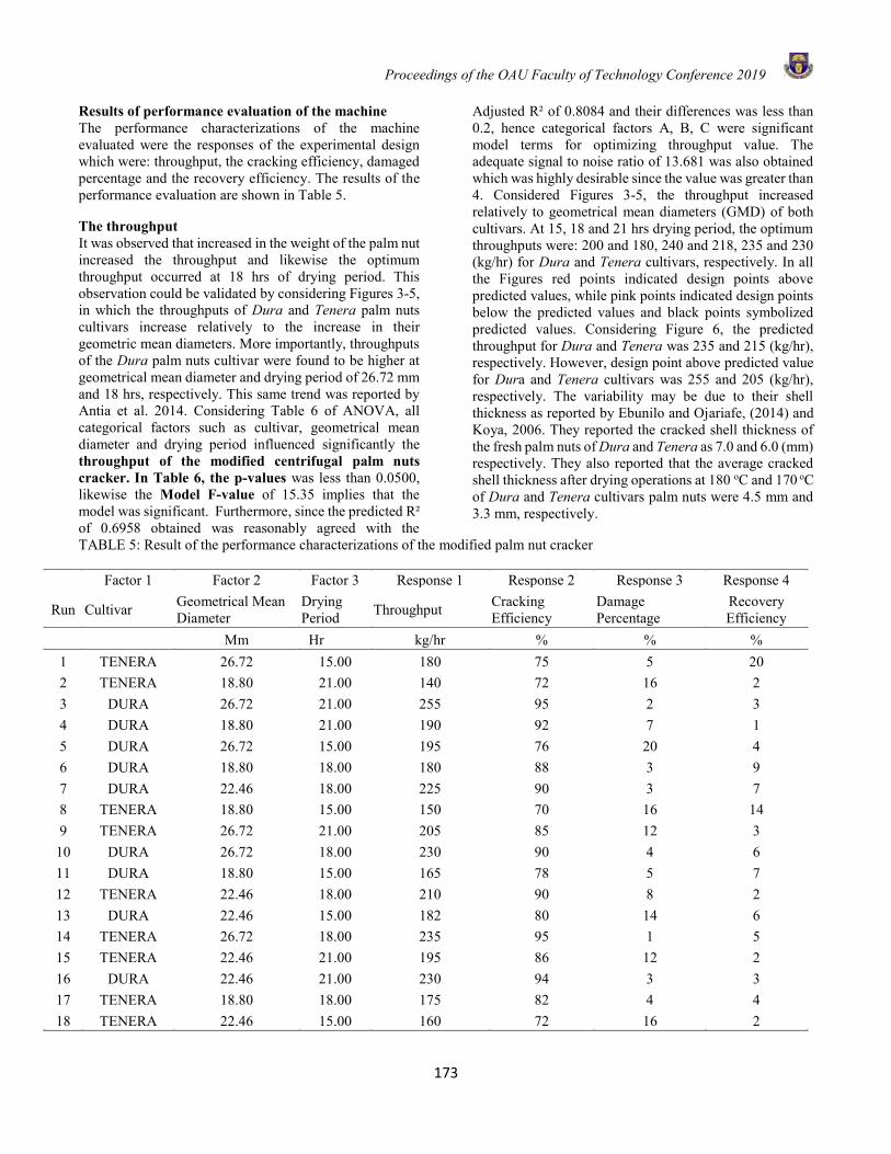
Proceedings of the OAU Faculty of Technology Conference 2019
173
Results of performance evaluation of the machine The performance characterizations of the machine evaluated were the responses of the experimental design which were: throughput, the cracking efficiency, damaged percentage and the recovery efficiency. The results of the performance evaluation are shown in Table 5.
The throughput It was observed that increased in the weight of the palm nut increased the throughput and likewise the optimum throughput occurred at 18 hrs of drying period. This observation could be validated by considering Figures 3-5, in which the throughputs of Dura and Tenera palm nuts cultivars increase relatively to the increase in their geometric mean diameters. More importantly, throughputs of the Dura palm nuts cultivar were found to be higher at geometrical mean diameter and drying period of 26.72 mm and 18 hrs, respectively. This same trend was reported by Antia et al. 2014. Considering Table 6 of ANOVA, all categorical factors such as cultivar, geometrical mean diameter and drying period influenced significantly the throughput of the modified centrifugal palm nuts cracker. In Table 6, the p-values was less than 0.0500, likewise the Model F-value of 15.35 implies that the model was significant. Furthermore, since the predicted R² of 0.6958 obtained was reasonably agreed with the
Adjusted R² of 0.8084 and their differences was less than 0.2, hence categorical factors A, B, C were significant model terms for optimizing throughput value. The adequate signal to noise ratio of 13.681 was also obtained which was highly desirable since the value was greater than 4. Considered Figures 3-5, the throughput increased relatively to geometrical mean diameters (GMD) of both cultivars. At 15, 18 and 21 hrs drying period, the optimum throughputs were: 200 and 180, 240 and 218, 235 and 230 (kg/hr) for Dura and Tenera cultivars, respectively. In all the Figures red points indicated design points above predicted values, while pink points indicated design points below the predicted values and black points symbolized predicted values. Considering Figure 6, the predicted throughput for Dura and Tenera was 235 and 215 (kg/hr), respectively. However, design point above predicted value for Dura and Tenera cultivars was 255 and 205 (kg/hr), respectively. The variability may be due to their shell thickness as reported by Ebunilo and Ojariafe, (2014) and Koya, 2006. They reported the cracked shell thickness of the fresh palm nuts of Dura and Tenera as 7.0 and 6.0 (mm) respectively. They also reported that the average cracked shell thickness after drying operations at 180 oC and 170 oC of Dura and Tenera cultivars palm nuts were 4.5 mm and 3.3 mm, respectively.
TABLE 5: Result of the performance characterizations of the modified palm nut cracker
Factor 1 Factor 2 Factor 3 Response 1 Response 2 Response 3 Response 4
Run Cultivar Geometrical Mean Diameter
Drying Period Throughput Cracking
Efficiency Damage Percentage
Recovery Efficiency
Mm Hr kg/hr % % % 1 TENERA 26.72 15.00 180 75 5 20 2 TENERA 18.80 21.00 140 72 16 2 3 DURA 26.72 21.00 255 95 2 3 4 DURA 18.80 21.00 190 92 7 1 5 DURA 26.72 15.00 195 76 20 4 6 DURA 18.80 18.00 180 88 3 9 7 DURA 22.46 18.00 225 90 3 7 8 TENERA 18.80 15.00 150 70 16 14 9 TENERA 26.72 21.00 205 85 12 3
10 DURA 26.72 18.00 230 90 4 6 11 DURA 18.80 15.00 165 78 5 7 12 TENERA 22.46 18.00 210 90 8 2 13 DURA 22.46 15.00 182 80 14 6 14 TENERA 26.72 18.00 235 95 1 5 15 TENERA 22.46 21.00 195 86 12 2 16 DURA 22.46 21.00 230 94 3 3 17 TENERA 18.80 18.00 175 82 4 4 18 TENERA 22.46 15.00 160 72 16 2
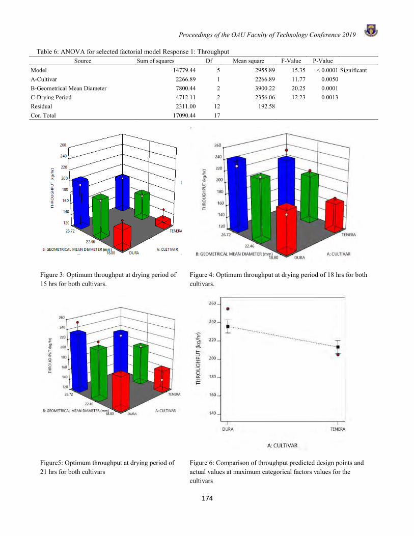
Proceedings of the OAU Faculty of Technology Conference 2019
174
Table 6: ANOVA for selected factorial model Response 1: Throughput Source Sum of squares Df Mean square F-Value P-Value
Model 14779.44 5 2955.89 15.35 < 0.0001 Significant A-Cultivar 2266.89 1 2266.89 11.77 0.0050
B-Geometrical Mean Diameter 7800.44 2 3900.22 20.25 0.0001
C-Drying Period 4712.11 2 2356.06 12.23 0.0013
Residual 2311.00 12 192.58
Cor. Total 17090.44 17
Figure 3: Optimum throughput at drying period of 15 hrs for both cultivars.
Figure 4: Optimum throughput at drying period of 18 hrs for both cultivars.
Figure5: Optimum throughput at drying period of 21 hrs for both cultivars
Figure 6: Comparison of throughput predicted design points and actual values at maximum categorical factors values for the cultivars
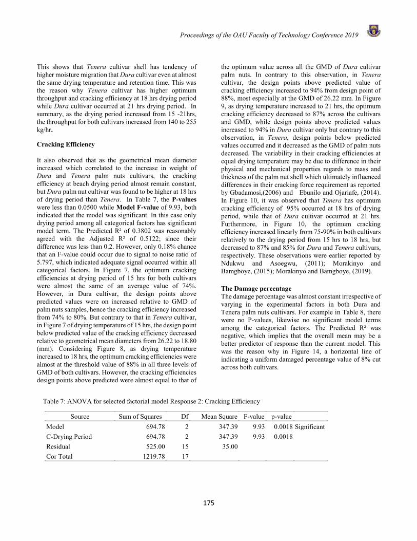
Proceedings of the OAU Faculty of Technology Conference 2019
175
This shows that Tenera cultivar shell has tendency of higher moisture migration that Dura cultivar even at almost the same drying temperature and retention time. This was the reason why Tenera cultivar has higher optimum throughput and cracking efficiency at 18 hrs drying period while Dura cultivar occurred at 21 hrs drying period. In summary, as the drying period increased from 15 -21hrs, the throughput for both cultivars increased from 140 to 255 kg/hr.
Cracking Efficiency
It also observed that as the geometrical mean diameter increased which correlated to the increase in weight of Dura and Tenera palm nuts cultivars, the cracking efficiency at beach drying period almost remain constant, but Dura palm nut cultivar was found to be higher at 18 hrs of drying period than Tenera. In Table 7, the P-values were less than 0.0500 while Model F-value of 9.93, both indicated that the model was significant. In this case only drying period among all categorical factors has significant model term. The Predicted R² of 0.3802 was reasonably agreed with the Adjusted R² of 0.5122; since their difference was less than 0.2. However, only 0.18% chance that an F-value could occur due to signal to noise ratio of 5.797, which indicated adequate signal occurred within all categorical factors. In Figure 7, the optimum cracking efficiencies at drying period of 15 hrs for both cultivars were almost the same of an average value of 74%. However, in Dura cultivar, the design points above predicted values were on increased relative to GMD of palm nuts samples, hence the cracking efficiency increased from 74% to 80%. But contrary to that in Tenera cultivar, in Figure 7 of drying temperature of 15 hrs, the design point below predicted value of the cracking efficiency decreased relative to geometrical mean diameters from 26.22 to 18.80 (mm). Considering Figure 8, as drying temperature increased to 18 hrs, the optimum cracking efficiencies were almost at the threshold value of 88% in all three levels of GMD of both cultivars. However, the cracking efficiencies design points above predicted were almost equal to that of
the optimum value across all the GMD of Dura cultivar palm nuts. In contrary to this observation, in Tenera cultivar, the design points above predicted value of cracking efficiency increased to 94% from design point of 88%, most especially at the GMD of 26.22 mm. In Figure 9, as drying temperature increased to 21 hrs, the optimum cracking efficiency decreased to 87% across the cultivars and GMD, while design points above predicted values increased to 94% in Dura cultivar only but contrary to this observation, in Tenera, design points below predicted values occurred and it decreased as the GMD of palm nuts decreased. The variability in their cracking efficiencies at equal drying temperature may be due to difference in their physical and mechanical properties regards to mass and thickness of the palm nut shell which ultimately influenced differences in their cracking force requirement as reported by Gbadamosi,(2006) and Ebunilo and Ojariafe, (2014). In Figure 10, it was observed that Tenera has optimum cracking efficiency of 95% occurred at 18 hrs of drying period, while that of Dura cultivar occurred at 21 hrs. Furthermore, in Figure 10, the optimum cracking efficiency increased linearly from 75-90% in both cultivars relatively to the drying period from 15 hrs to 18 hrs, but decreased to 87% and 85% for Dura and Tenera cultivars, respectively. These observations were earlier reported by Ndukwu and Asoegwu, (2011); Morakinyo and Bamgboye, (2015); Morakinyo and Bamgboye, (2019).
The Damage percentage The damage percentage was almost constant irrespective of varying in the experimental factors in both Dura and Tenera palm nuts cultivars. For example in Table 8, there were no P-values, likewise no significant model terms among the categorical factors. The Predicted R² was negative, which implies that the overall mean may be a better predictor of response than the current model. This was the reason why in Figure 14, a horizontal line of indicating a uniform damaged percentage value of 8% cut across both cultivars.
Table 7: ANOVA for selected factorial model Response 2: Cracking Efficiency
Source Sum of Squares Df Mean Square F-value p-value
Model 694.78 2 347.39 9.93 0.0018 Significant C-Drying Period 694.78 2 347.39 9.93 0.0018
Residual 525.00 15 35.00
Cor Total 1219.78 17
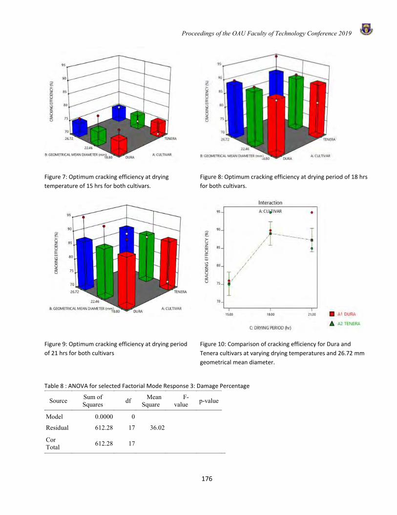
Proceedings of the OAU Faculty of Technology Conference 2019
176
Figure 7: Optimum cracking efficiency at drying
temperature of 15 hrs for both cultivars.
Figure 8: Optimum cracking efficiency at drying period of 18 hrs
for both cultivars.
Figure 9: Optimum cracking efficiency at drying period
of 21 hrs for both cultivars
Figure 10: Comparison of cracking efficiency for Dura and
Tenera cultivars at varying drying temperatures and 26.72 mm
geometrical mean diameter.
Table 8 : ANOVA for selected Factorial Mode Response 3: Damage Percentage
Source Sum of Squares df Mean
Square F-value p-value
Model 0.0000 0
Residual 612.28 17 36.02
Cor Total 612.28 17
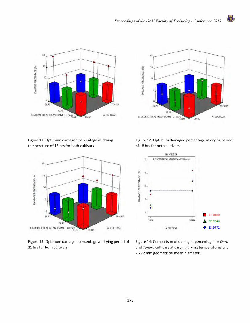
Proceedings of the OAU Faculty of Technology Conference 2019
177
Figure 11: Optimum damaged percentage at drying
temperature of 15 hrs for both cultivars.
Figure 12: Optimum damaged percentage at drying period
of 18 hrs for both cultivars.
Figure 13: Optimum damaged percentage at drying period of
21 hrs for both cultivars
Figure 14: Comparison of damaged percentage for Dura
and Tenera cultivars at varying drying temperatures and
26.72 mm geometrical mean diameter.
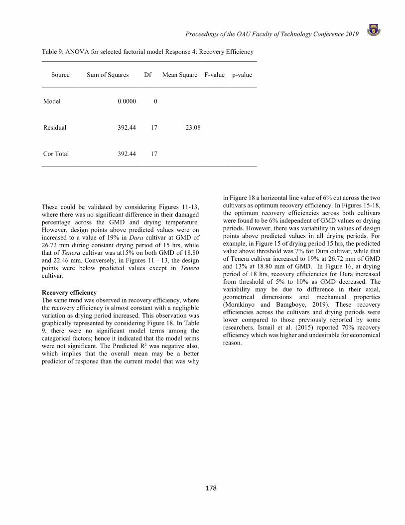
Proceedings of the OAU Faculty of Technology Conference 2019
178
Table 9: ANOVA for selected factorial model Response 4: Recovery Efficiency
Source Sum of Squares Df Mean Square F-value p-value
Model 0.0000 0
Residual 392.44 17 23.08
Cor Total 392.44 17
These could be validated by considering Figures 11-13, where there was no significant difference in their damaged percentage across the GMD and drying temperature. However, design points above predicted values were on increased to a value of 19% in Dura cultivar at GMD of 26.72 mm during constant drying period of 15 hrs, while that of Tenera cultivar was at15% on both GMD of 18.80 and 22.46 mm. Conversely, in Figures 11 - 13, the design points were below predicted values except in Tenera cultivar.
Recovery efficiency The same trend was observed in recovery efficiency, where the recovery efficiency is almost constant with a negligible variation as drying period increased. This observation was graphically represented by considering Figure 18. In Table 9, there were no significant model terms among the categorical factors; hence it indicated that the model terms were not significant. The Predicted R² was negative also, which implies that the overall mean may be a better predictor of response than the current model that was why
in Figure 18 a horizontal line value of 6% cut across the two cultivars as optimum recovery efficiency. In Figures 15-18, the optimum recovery efficiencies across both cultivars were found to be 6% independent of GMD values or drying periods. However, there was variability in values of design points above predicted values in all drying periods. For example, in Figure 15 of drying period 15 hrs, the predicted value above threshold was 7% for Dura cultivar, while that of Tenera cultivar increased to 19% at 26.72 mm of GMD and 13% at 18.80 mm of GMD. In Figure 16, at drying period of 18 hrs, recovery efficiencies for Dura increased from threshold of 5% to 10% as GMD decreased. The variability may be due to difference in their axial, geometrical dimensions and mechanical properties (Morakinyo and Bamgboye, 2019). These recovery efficiencies across the cultivars and drying periods were lower compared to those previously reported by some researchers. Ismail et al. (2015) reported 70% recovery efficiency which was higher and undesirable for economical reason.
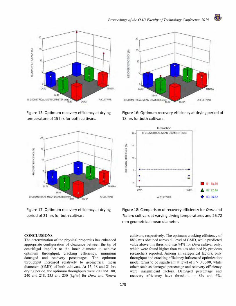
Proceedings of the OAU Faculty of Technology Conference 2019
179
Figure 15: Optimum recovery efficiency at drying
temperature of 15 hrs for both cultivars.
Figure 16: Optimum recovery efficiency at drying period of
18 hrs for both cultivars.
Figure 17: Optimum recovery efficiency at drying
period of 21 hrs for both cultivars
Figure 18: Comparison of recovery efficiency for Dura and
Tenera cultivars at varying drying temperatures and 26.72
mm geometrical mean diameter.
CONCLUSIONS The determination of the physical properties has enhanced appropriate configuration of clearance between the tip of centrifugal impeller to the inner diameter to achieve optimum throughput, cracking efficiency, minimum damaged and recovery percentages. The optimum throughput increased relatively to geometrical mean diameters (GMD) of both cultivars. At 15, 18 and 21 hrs drying period, the optimum throughputs were 200 and 180, 240 and 218, 235 and 230 (kg/hr) for Dura and Tenera
cultivars, respectively. The optimum cracking efficiency of 88% was obtained across all level of GMD, while predicted value above this threshold was 94% for Dura cultivar only, which were found higher than values obtained by previous researchers reported. Among all categorical factors, only throughput and cracking efficiency influenced optimization model terms to be significant at level of P> 0.0500, while others such as damaged percentage and recovery efficiency were insignificant factors. Damaged percentage and recovery efficiency have threshold of 8% and 6%,
Proceedings of the OAU Faculty of Technology Conference 2019
180
respectively. Hence, the determination of physical properties and inferential statistical analysis, before embarking on development of the modified centrifugal palm nuts cracker improved performance characteristics and reduced damaged percentages. ACKNOWLEDGEMENT The author acknowledged the student in person of Chijioke Godwin Nwankpa, who contributed enormously in area of machine construction and data collection and technical staff of Department of Food Science and Technology Faculty of Technology, Obafemi Awolowo University, Ile-Ife.
REFERENCES Adebayo, A. A., Development and performance evaluation
of a motorized palm-nut cracking machine. Proceedings of the Annual Conference of the Nigerian Institution of Agricultural Engineers, 26, 326-330, 2004.
Adejugbe, T., Oyegunwa, O. A., Iliya, D. D., Aigbogun, J. O, Oyelami A. T., Olusunle S. O. O., Design and Development of an Improved Palm Kernel Shelling Machine and Separator. Physical Science International Journal, 14(3): 1-9, 2017.
Adzimah, S. K. and Seckley, E., Modification in the design of an already existing palm nut - fibre separator. AfricaJournal of Environmental Science and Technology. 3(11): 387-398, 2009.
Antia, O.O., Olusunde, W., Offiong, A., Determination of optimum moisture content of palm nut cracking for efficient production of whole kernel. Nigeria Journal of Technological Development. 11(2: 27-30), 2014.
Davies, R. M., Physical and mechanical properties of palm fruit, kernel and nut. Journal of Agricultural Technology 8(7):2147-2156, 2012.
Ebunilo, P., Ojariafe, G., An experimental study on the use of temperaturefor effective separation of cracked palm nuts from their shells, Proceedings of the World Congress on Engineering and Computer Science, WCECS , San Francisco, USA, Vol II, 22-24, 2014.
Emeka, V. E., Olomu, J. M., Nutritional evaluation of palm kernel meal types: proximate composition and metabolizable energy values. African Journal of Biotechnology, 6(21), 2484-2486, 2007.
FAO, Small-scale palm oil processing in Africa. FAO AGRICULTURAL SERVICES BULLETIN 148, ROME. ISSN 1010-1365, ISBN-92-5-104859-23, 2002.
Gbabo, A., Gana, I. M., Amoto, M. S. Design, fabrication and testing of a millet thresher. Net Journal of Agricultural Science 1(4): 100-106, 2013.
Gbadamosi, L., Some engineering properties of palm kernel seeds. Journal of Agricultural Engineering and Technology, 14, 58 – 67, 2006.
Ismail, S. O., Ojolo, S. J., Orisaleye, J. I., Adediran, A. A., Fajuyitan, O. O., Design and development of an improved palm kernel shelling and sorting machine European International Journal of Science and Technology, 4(2):226-240, 2015.
Khurmi, R .S. Engineering mechanics (Applied Mechanics), 2005 reprinted Edition, published by S. Chand & Company Ltd, 7361, Ram Nagar, New Delhi-110055, India, 2005.
Khurmi, R .S., Gupta, J.K., Machine Design, S.I Unit Edition, New Delhi, India, 24-56.Koya, O.A, 2006. Palm nuts cracking under repeated impact load, Journal of Applied Science. 6(1):2471-2475, 2006.
Morakinyo, T. A., Bamgboye, A. I., Effects of Age on some physical properties of oil palm fruitlets. International Journal of Agricultural Engineering Research (CIGR). 17(3): 342-352, 2015.
Morakinyo, T. A., Bamgboye, A. I., Some engineering properties of palm nuts, kernel shell, fibre and woods for effective mill equipment design. American Journal of Material Science and Application. 7(1):1-7, 2019.
Mutsaers, H.T.W., The challenge of the oil palm: using degraded land for its cultivation. Journal of Outlook on Agriculture SAGE publication. DIO: 10: 1177/0030727019858720 Volume xx(x): 1-8, 2019.
Ndukwu, M. C., Asoegwu, S. N., A mathematical model for predicting the cracking efficiency of vertical-shaft centrifugal palm nut cracker. Research Agricultural Engineering. 57: 110–115, 2011.
Stat-Ease, Inc., Design-Expert® Software is a registered trademark of Stat-Ease, Inc.
Privacy Policy. Terms of Service. 1300 Godward St NE, Suite 6400, Minneapolis, MN 55413, 2019.
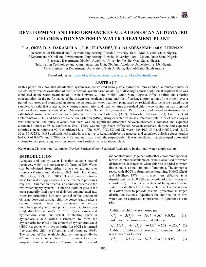
Proceedings of the OAU Faculty of Technology Conference 2019
181
DEVELOPMENT AND PERFORMANCE EVALUATION OF AN AUTOMATED CHLORINATION SYSTEM IN WATER TREATMENT PLANT
I. A, OKE2, D. A. DARAMOLA1 , J. B., ELUSADE3, T.A, ALADESANMI4 and S. LUKMAN5 1Department of Electrical and Electronic Engineering, Elizade University, Ilara - Mokin, Ondo State, Nigeria
2 Department of Civil and Environmental Engineering, Elizade University, Ilara – Mokin, Ondo State, Nigeria 3Pharmacy Department, Obafemi Awolowo University, Ile- Ife, Osun State, Nigeria
4Information Technology and Communications Unit, Obafemi Awolowo University, Ile- Ife, Nigeria 5 Civil Engineering Department, University of Hafr Al-Batin, Hafr Al-Batin, Saudi Arabia
E-mail Addresses: [email protected] or [email protected] ;
ABSTRACT
In this paper, an automated disinfection system was constructed from plastic cylindrical tanks and an automatic controller system. Performance evaluation of the disinfection system based on ability to discharge chlorine solution at required time was conducted at the water treatment of Elizade University, Ilara- Mokin, Ondo State, Nigeria. Effect of time and chlorine concentration on the performance of the system was evaluated using analysis of variance. Application of the system over a period was tested and monitored on-site at the institutional water treatment plant based on residual chlorine in the treated water samples. A model that relates added chlorine concentration and treatment time to residual chlorine concentration was proposed and developed using statistical and Microsoft Excel Solver (MES) methods. Performance and model evaluations were established using statistical methods (Akaike Information Criterion, (AIC), Schwartz Criterion (SC), Coefficient of Determination (CD) and Model of Selection Criterion (MSC)) using expected value as a reference data. A brief cost analysis was conducted. The study revealed that there was no significant difference between observed automated and expected automated timers at 95 % confidence level. There was no significant difference between observed chlorine and expected chlorine concentrations at 99 % confidence level. The MSC, AIC, SC and CD were 44.0, 10.0, 33.0 and 0.9679, and 43, 12, 35 and 0.9523 for MES and statistical methods, respectively. Relationship between actual and calculated chlorine concentration had CD of 0.7078 and 0.7076 for MES and statistical methods, respectively. It was concluded that developed automated chlorinator is a promising device in conventional surface water treatment plant. Keywords: Chlorination, Automated Device, Surface Water, Statistical Evaluation, Institutional water supply system INTRODUCTION Adequate and quality water is major valuable natural resources, which is important to all forms of life. Water can be obtained from either surface or groundwater sources (Martins and Martins, 1993; John De Zuane, 1996; Gray, 1999; JMP, 2017). The difference between these two water supply systems is the treatment processes required. Disinfection process is a common process to the two water supply systems. Chlorine (solid or gas) is the most generally used agent to disinfect contaminated raw water (chlorination). Stringent control of the amount of chlorine dose and residual chlorine concentration after a certain contact time is necessary to ensure microbiologically safe and potable water. Chlorine gas (Cl2) dissolves in water to form hypochlorous and hydrochloric acid. The actual disinfecting agent is hypochlorous acid which dissiociates to form the hypochlorite ion (OCl-). The amount of hypochlorous acid (HOCl) together with hypochlorite ion (OCl-) is termed free available chlorine (Viessman and Hammer, 1993). The residual of free available chlorine must generally be 0.5 mg/l after a contact time of 30 minutes to ensure properly disinfected water. Chlorine in the form of
monochloramine (together with other chloramine species) termed combined available chlorine is also used for water disinfection. It is formed when chlorine is added to water that contains a small amount of ammonia. The ammonia reacts with HOCl to form monochloramine, NH2Cl (Steel and McGhee, 1979). It is much less effective as a disinfectant than HOCl (the same order of effectiveness as chlorite ion). It has the advantage of being much more stable in water than free available chlorine. For this reason it is often used to provide residual protection in larger distribution systems. Equations for chlorination of raw water can be expressed as presented in Equations (1) to (6): Addition of chlorine as chlorine gas:
−+ ++→+ OClHHClOHCl 333 22 (1) Addition of chlorine as as solid chlorine:
−−+ ++→+ OClOHCaOHOClCa 2)( 222 (2)
Addition of chlorine in presence of ammonia, chlorine reactions are as follows:
−+ ++→+ OClHHClOHCl 333 22 (3)
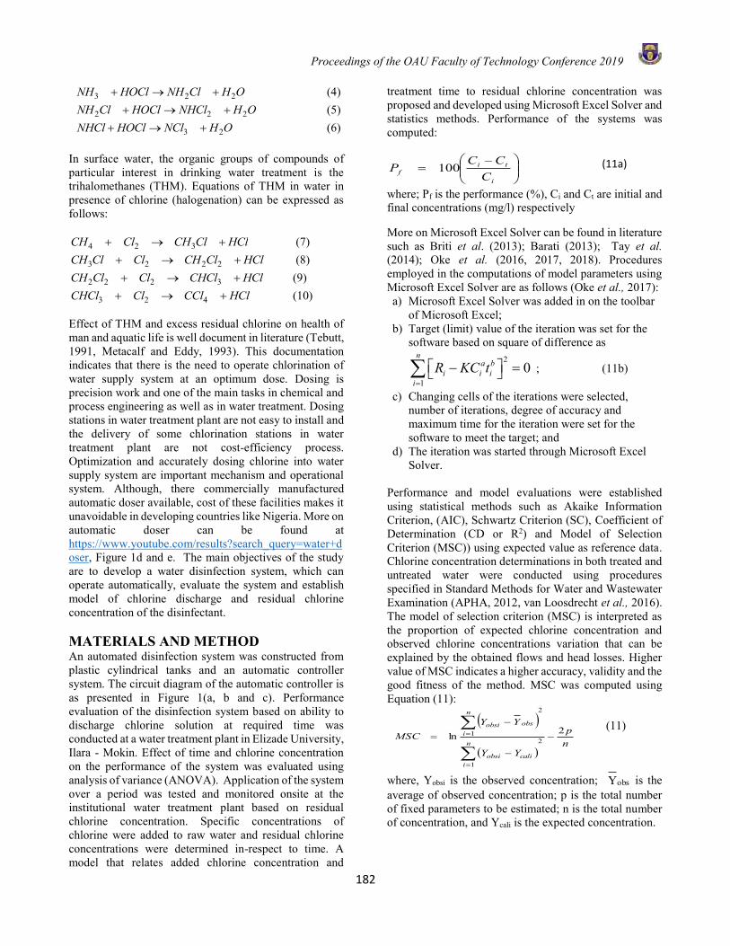
Proceedings of the OAU Faculty of Technology Conference 2019
182
3 2 2NH HOCl NH Cl H O+ → + (4)
2 2 2NH Cl HOCl NHCl H O+ → + (5)
3 2NHCl HOCl NCl H O+ → + (6)
In surface water, the organic groups of compounds of particular interest in drinking water treatment is the trihalomethanes (THM). Equations of THM in water in presence of chlorine (halogenation) can be expressed as follows:
4 2 3CH Cl CH Cl HCl+ → + (7)
3 2 2 2CH Cl Cl CH Cl HCl+ → + (8)
2 2 2 3CH Cl Cl CHCl HCl+ → + (9)
3 2 4CHCl Cl CCl HCl+ → + (10) Effect of THM and excess residual chlorine on health of man and aquatic life is well document in literature (Tebutt, 1991, Metacalf and Eddy, 1993). This documentation indicates that there is the need to operate chlorination of water supply system at an optimum dose. Dosing is precision work and one of the main tasks in chemical and process engineering as well as in water treatment. Dosing stations in water treatment plant are not easy to install and the delivery of some chlorination stations in water treatment plant are not cost-efficiency process. Optimization and accurately dosing chlorine into water supply system are important mechanism and operational system. Although, there commercially manufactured automatic doser available, cost of these facilities makes it unavoidable in developing countries like Nigeria. More on automatic doser can be found at https://www.youtube.com/results?search_query=water+doser, Figure 1d and e. The main objectives of the study are to develop a water disinfection system, which can operate automatically, evaluate the system and establish model of chlorine discharge and residual chlorine concentration of the disinfectant. MATERIALS AND METHOD An automated disinfection system was constructed from plastic cylindrical tanks and an automatic controller system. The circuit diagram of the automatic controller is as presented in Figure 1(a, b and c). Performance evaluation of the disinfection system based on ability to discharge chlorine solution at required time was conducted at a water treatment plant in Elizade University, Ilara - Mokin. Effect of time and chlorine concentration on the performance of the system was evaluated using analysis of variance (ANOVA). Application of the system over a period was tested and monitored onsite at the institutional water treatment plant based on residual chlorine concentration. Specific concentrations of chlorine were added to raw water and residual chlorine concentrations were determined in-respect to time. A model that relates added chlorine concentration and
treatment time to residual chlorine concentration was proposed and developed using Microsoft Excel Solver and statistics methods. Performance of the systems was computed:
−=
i
tif C
CCP 100 (11a)
where; Pf is the performance (%), Ci and Ct are initial and final concentrations (mg/l) respectively More on Microsoft Excel Solver can be found in literature such as Briti et al. (2013); Barati (2013); Tay et al. (2014); Oke et al. (2016, 2017, 2018). Procedures employed in the computations of model parameters using Microsoft Excel Solver are as follows (Oke et al., 2017): a) Microsoft Excel Solver was added in on the toolbar
of Microsoft Excel; b) Target (limit) value of the iteration was set for the
software based on square of difference as2
10
na b
i i ii
R KC t=
− = ; (11b)
c) Changing cells of the iterations were selected, number of iterations, degree of accuracy and maximum time for the iteration were set for the software to meet the target; and
d) The iteration was started through Microsoft Excel Solver.
Performance and model evaluations were established using statistical methods such as Akaike Information Criterion, (AIC), Schwartz Criterion (SC), Coefficient of Determination (CD or R2) and Model of Selection Criterion (MSC)) using expected value as reference data. Chlorine concentration determinations in both treated and untreated water were conducted using procedures specified in Standard Methods for Water and Wastewater Examination (APHA, 2012, van Loosdrecht et al., 2016). The model of selection criterion (MSC) is interpreted as the proportion of expected chlorine concentration and observed chlorine concentrations variation that can be explained by the obtained flows and head losses. Higher value of MSC indicates a higher accuracy, validity and the good fitness of the method. MSC was computed using Equation (11):
( )
( )np
YY
YYMSC
n
icaliobsi
n
iobsobsi
2ln 2
1
2
1 −
−
−
=
=
= (11)
where, Yobsi is the observed concentration; obsY is the average of observed concentration; p is the total number of fixed parameters to be estimated; n is the total number of concentration, and Ycali is the expected concentration.
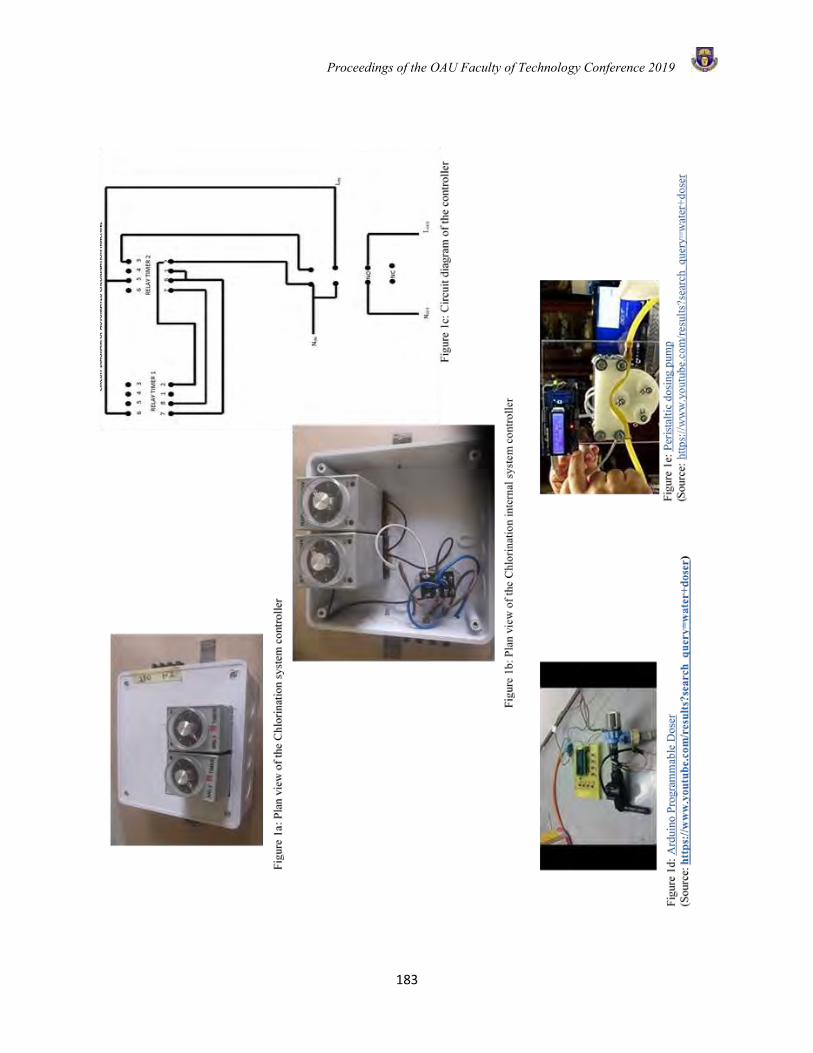
Proceedings of the OAU Faculty of Technology Conference 2019
183
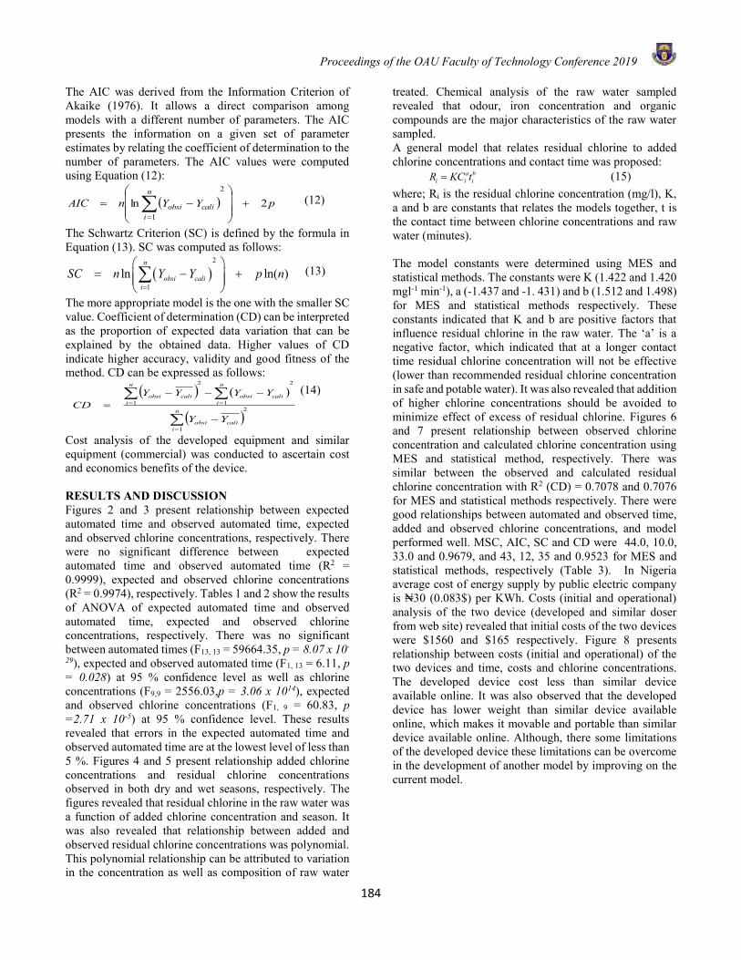
Proceedings of the OAU Faculty of Technology Conference 2019
184
The AIC was derived from the Information Criterion of Akaike (1976). It allows a direct comparison among models with a different number of parameters. The AIC presents the information on a given set of parameter estimates by relating the coefficient of determination to the number of parameters. The AIC values were computed using Equation (12):
( ) pYYnAICn
icaliobsi 2ln
2
1
+
−= =
(12)
The Schwartz Criterion (SC) is defined by the formula in Equation (13). SC was computed as follows:
( )2
1ln ln( )
n
obsi calii
SC n Y Y p n=
= − +
(13)
The more appropriate model is the one with the smaller SC value. Coefficient of determination (CD) can be interpreted as the proportion of expected data variation that can be explained by the obtained data. Higher values of CD indicate higher accuracy, validity and good fitness of the method. CD can be expressed as follows:
( ) ( )
( )2
1
2
1
2
1
=
==
−
−−−=
n
icaliobsi
n
icaliobsi
n
icaliobsi
YY
YYYYCD
(14)
Cost analysis of the developed equipment and similar equipment (commercial) was conducted to ascertain cost and economics benefits of the device.
RESULTS AND DISCUSSION Figures 2 and 3 present relationship between expected automated time and observed automated time, expected and observed chlorine concentrations, respectively. There were no significant difference between expected automated time and observed automated time (R2 = 0.9999), expected and observed chlorine concentrations (R2 = 0.9974), respectively. Tables 1 and 2 show the results of ANOVA of expected automated time and observed automated time, expected and observed chlorine concentrations, respectively. There was no significant between automated times (F13, 13 = 59664.35, p = 8.07 x 10-
29), expected and observed automated time (F1, 13 = 6.11, p = 0.028) at 95 % confidence level as well as chlorine concentrations (F9,9 = 2556.03,p = 3.06 x 10¹⁴), expected and observed chlorine concentrations (F1, 9 = 60.83, p =2.71 x 10⁻⁵) at 95 % confidence level. These results revealed that errors in the expected automated time and observed automated time are at the lowest level of less than 5 %. Figures 4 and 5 present relationship added chlorine concentrations and residual chlorine concentrations observed in both dry and wet seasons, respectively. The figures revealed that residual chlorine in the raw water was a function of added chlorine concentration and season. It was also revealed that relationship between added and observed residual chlorine concentrations was polynomial. This polynomial relationship can be attributed to variation in the concentration as well as composition of raw water
treated. Chemical analysis of the raw water sampled revealed that odour, iron concentration and organic compounds are the major characteristics of the raw water sampled. A general model that relates residual chlorine to added chlorine concentrations and contact time was proposed:
a bi i iR KC t= (15)
where; Ri is the residual chlorine concentration (mg/l), K, a and b are constants that relates the models together, t is the contact time between chlorine concentrations and raw water (minutes). The model constants were determined using MES and statistical methods. The constants were K (1.422 and 1.420 mgl-1 min-1), a (-1.437 and -1. 431) and b (1.512 and 1.498) for MES and statistical methods respectively. These constants indicated that K and b are positive factors that influence residual chlorine in the raw water. The ‘a’ is a negative factor, which indicated that at a longer contact time residual chlorine concentration will not be effective (lower than recommended residual chlorine concentration in safe and potable water). It was also revealed that addition of higher chlorine concentrations should be avoided to minimize effect of excess of residual chlorine. Figures 6 and 7 present relationship between observed chlorine concentration and calculated chlorine concentration using MES and statistical method, respectively. There was similar between the observed and calculated residual chlorine concentration with R2 (CD) = 0.7078 and 0.7076 for MES and statistical methods respectively. There were good relationships between automated and observed time, added and observed chlorine concentrations, and model performed well. MSC, AIC, SC and CD were 44.0, 10.0, 33.0 and 0.9679, and 43, 12, 35 and 0.9523 for MES and statistical methods, respectively (Table 3). In Nigeria average cost of energy supply by public electric company is ₦30 (0.083$) per KWh. Costs (initial and operational) analysis of the two device (developed and similar doser from web site) revealed that initial costs of the two devices were $1560 and $165 respectively. Figure 8 presents relationship between costs (initial and operational) of the two devices and time, costs and chlorine concentrations. The developed device cost less than similar device available online. It was also observed that the developed device has lower weight than similar device available online, which makes it movable and portable than similar device available online. Although, there some limitations of the developed device these limitations can be overcome in the development of another model by improving on the current model.
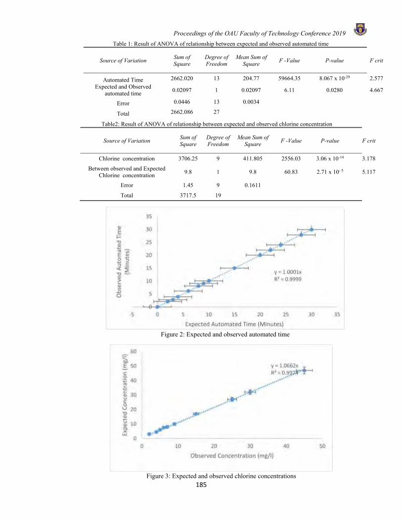
Proceedings of the OAU Faculty of Technology Conference 2019
185
Figure 3: Expected and observed chlorine concentrations
Table 1: Result of ANOVA of relationship between expected and observed automated time
Source of Variation Sum of Square
Degree of Freedom
Mean Sum of Square F -Value P-value F crit
Automated Time 2662.020 13 204.77 59664.35 8.067 x 10⁻²⁹ 2.577 Expected and Observed
automated time 0.02097 1 0.02097 6.11 0.0280 4.667
Error 0.0446 13 0.0034
Total 2662.086 27
Table2: Result of ANOVA of relationship between expected and observed chlorine concentration
Source of Variation Sum of Square
Degree of Freedom
Mean Sum of Square F -Value P-value F crit
Chlorine concentration 3706.25 9 411.805 2556.03 3.06 x 10⁻¹⁴ 3.178
Between observed and Expected Chlorine concentration 9.8 1 9.8 60.83 2.71 x 10- 5 5.117
Error 1.45 9 0.1611
Total 3717.5 19
Figure 2: Expected and observed automated time
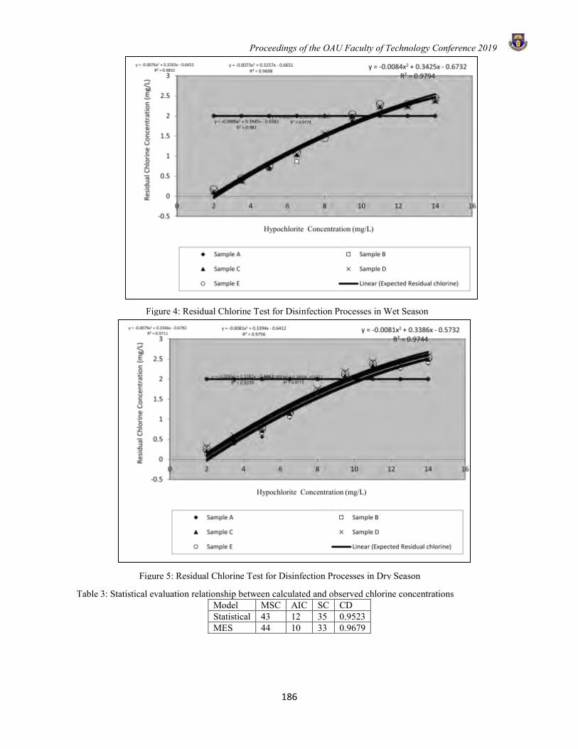
Proceedings of the OAU Faculty of Technology Conference 2019
186
Table 3: Statistical evaluation relationship between calculated and observed chlorine concentrations
Model MSC AIC SC CD Statistical 43 12 35 0.9523 MES 44 10 33 0.9679
Figure 4: Residual Chlorine Test for Disinfection Processes in Wet Season
Figure 5: Residual Chlorine Test for Disinfection Processes in Dry Season
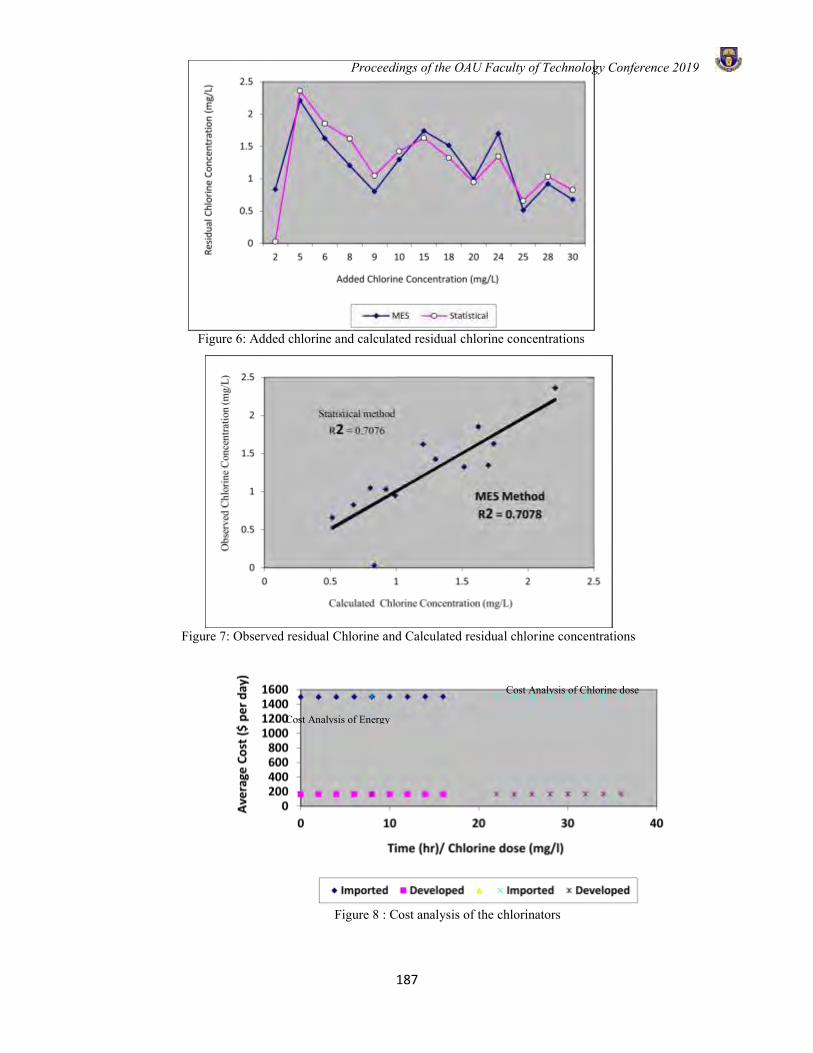
Proceedings of the OAU Faculty of Technology Conference 2019
187
Figure 6: Added chlorine and calculated residual chlorine concentrations
Figure 7: Observed residual Chlorine and Calculated residual chlorine concentrations
Figure 8 : Cost analysis of the chlorinators
Cost Analysis of Energy
Cost Analysis of Chlorine dose
Proceedings of the OAU Faculty of Technology Conference 2019
188
CONCLUSION It can be concluded based on the study that: Performance of the automated raw water chlorination
system was adequate (no significant differences between observed automated and expected automated time, expected and observed residual chlorine concentrations),
Predictions of the proposed models (based on MES and statistical methods) were good based on MSC, AIC, CD and SC.
REFERENCES Akaike, H. (1976). An information criterion (AIC), Math.
Sci. 14,1-5. APHA, (2012) Standard Method for the Examination of
Water and Wastewater, 22nd Edn., America Water Works Association and Water Pollution Control Federation, Washington DC.
Barati, R. (2013) Application of Excel solver for parameter estimation of the nonlinear Muskingum models. Korean Society of Civil Engineer, Journal of Civil Engineering, 17(5), 1139-1148
Briti S.'S.; Preetam B.; Ajeet K, P.;Jarken Band Pallavi S. (2013). Use of excel-solver as an optimization tool in design of pipe network. International Journal of Hydraulic Engineering, 2(4), 59-63
Gray, N. F. (1999). Water Technology: An introduction for Environmental Scientists and Engineers, 1st edn, Arnold and John Wiley and Sons, New York.
JMP (2017) update Progress on sanitation and drinking-water - 2017 update (http://www.who.int/about/licensing/copyright_form/en/. Access on 23th March 2019
John De Zuane, P.E (1996). Handbook of Drinking Water Quality. 2nd Edn, Van Nostrand Reinhold, Toronto.
Martins, J. E. and Martins, T. E.(1993).Technologies For Small Water And Wastewater Systems, 2nd edn, Van Nostrand Reinhold Company, New York.
Metcalf and Eddy Inc. (1991) Wastewater Engineering Treatment Disposal and Reuse, 3rd edn, McGraw-Hill Book Company, New York.
Oke, I. A, S. Lukman, J. S. Amoko and E. O. Fehintola (2018) An Evaluation Of Solutions To Moment Method Of Biochemical Oxygen Demand Kinetics. Nigerian Journal of Technology (NIJOTECH) 37,(1), 1 – 12
Oke, I. A. ; Ismail, A. ; Lukman, S. ; S. O. Ojo, O. O. Adeosun, and M. O. Nwude (2016). Economics and Statistical Evaluations of Using Microsoft Excel Solver in Pipe Network Analysis. J. Pipeline Syst. Eng. 7(4): 06016002-1- 9
Oke, I. A.; Lukman, S. and Ismail, A (2017). Development And Performance Evaluation Of A New Numerical Model For Groundwater Recharge Estimation. Nigeria Journal of Engineering , 23(2), 56 -65.
Steel, E.W. and McGhee, J.T. (1979). Water Supply and Sewerage, 1st edn, McGraw Hill Book Company, Tokyo.
Tay,K G; Kek, S. L. and Rosmila A. K (2014). Solving non-linear systems by newton's method using spreadsheet excel. Http://recsam.edu.my/cosmed! cosmed 09/AbstractsFullPa pers2009/ Abstract/Ma t hematics%20Parallel%20PDF/Full%20Paper/M3 3.pdE Accessed on21stDecember2014
Tebbutt, T. H. Y. (1991). Principles of Water Quality Control, 3rd edn, Pergamon Press, Oxford.
van Loosdrecht, M.C.M., Nielsen, P.H.,Lopez-Vazquez, C.M., Brdjanovic, D., (2016). Experimental Methods in Wastewater Treatment. 1st Edition, International Water Publishing Alliance House, London.
Viessman, W, and Hammer, M. (1993). Water Supply and Pollution Control. New York: Harper Collins College Publishers.
Proceedings of the OAU Faculty of Technology Conference 2019
189
DEVELOPMENT OF A LABORATORY ROTARY SHAFT TORQUEMETER
Ajayi O. K.* and Ghazal T. O. Department of Mechanical Engineering, Obafemi Awolowo University, Ile Ife
*Email of Corresponding Author: [email protected]
ABSTRACT This load cell torquemeter design is based on the principle of strain gauges, The load cell was with bonded strain gauges was used and a microcontroller was used for processing signal sensed by the load cell. When the component is loaded, strains develop and are transmitted to the foil grid and thus electrical resistance of the grid changes in proportion to the load-induced strain. Results were displayed on a LCD screen and also acquired on a PC through a USB serial port using Arduino software GUI. Initial readings of known weights and torques were used to calibrate the equipment. New readings were obtained for weights and torques and the readings showed improvement and correctness over the reading taking before calibration. The error in weight and torque value vis a vis measured value was close to unity, while performance analysis at 95% confidence level showed that there is no significance difference in these values. Therefore, the developed torquemeter is cable of being used for the laboratory experimental purpose for student projects and learning.
Keywords: Torquemeter, Load cell, Strain gauge, Arduino
INTRODUCTION Many of the machines that we use in everyday life employ rotating shafts to transmit mechanical power. Manufacturers are faced with competitive pressure to improve efficiency as well as product quality. This drives the desire to measure and control this mechanical power in the industrial environment. A means to measure the power transmitted is to measure the torque and the rotational velocity of the shaft. Derived from the latin word ‘torquere’ meaning 'to twist', torque is part of our everyday life (Tullis, 2000). Torque measurement instruments are used extensively on agricultural and industrial processing machinery (Husak et al., 2002). Normally the performance of rotating drives is described by torque and rotational speed and there is the need to accurately measure rotational speed and torque. There is a need for an economical, universal, continuous range, precision torque meter (Buchele, 1955). To determine shaft torque in rotating machinery, a common technique is the measurement of the twist in a torque bar inserted between the source and load. The use of strain gages mounted on the torque bar to measure twist is one of the means used to measure the torque of the rotating devices while slip rings or telemetry is used to transfer the strain gauge outputs. Field performance testing and monitoring with the aid of torque meter device is essential in turbo-machinery to assess its current condition. For example, the objective of field testing gas turbine driven compressor sets is typically to verify acceptance criteria such as heat rate, specific fuel consumption, turbine shaft power and compressor gas power (Lebow, 1999).
Generally, performance testing is done on a machine to determine the accuracy and correctness of its output against predetermined standard or function. Piotr (2014) presented a method of measurement for a complex system comprising a cooling system to measure the strain in a charge air cooler during an experiment for specific thermal cycle tests. Wheatstone bridge arrangement was used to investigate noise level for a sensor measurement system to ensure accurate measurement. The result shows the AC-excitation to have hiugher noise level than the DC-excitation (Khan et al. 2014). Earlier, a ‘V’ shape strain gauge was attached to the end of a shaft coupled with a slip-ring assembly for a more accurate and simple arrangement torque measurement (Muftah and Haris, 2011). More recently, a torque transducer based on twist angle deformation for torque measurement using wireless transmission was studied (Ali et al, 2018). The objective of this work was to develop a torquemeter which is suitable for laboratory experiments and students project work in a university. The principle is based on the strain gauge ability to measure force which can be converted to both weight and torque. METHODS These section discusses the sensor, the microprocessor and the data acquisition units used for this study. The sensor Load cells are electromechanical devices used to measure force, stress and strain in a system or a surface, with the aid
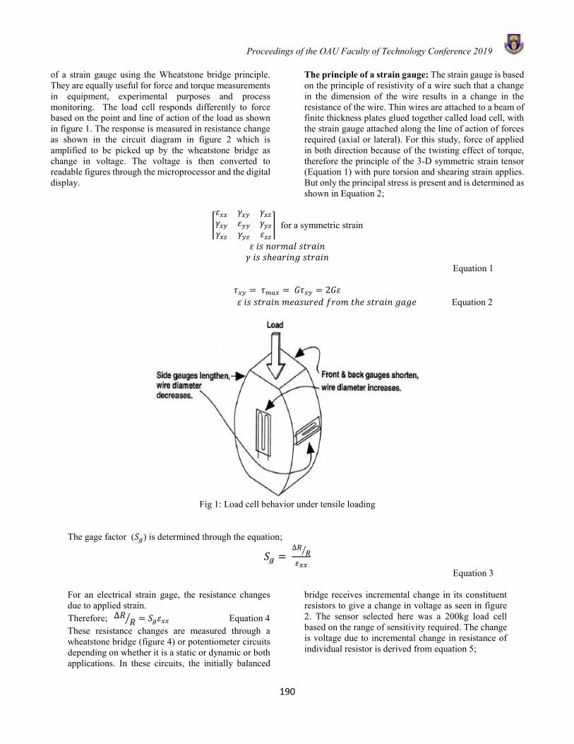
Proceedings of the OAU Faculty of Technology Conference 2019
190
of a strain gauge using the Wheatstone bridge principle. They are equally useful for force and torque measurements in equipment, experimental purposes and process monitoring. The load cell responds differently to force based on the point and line of action of the load as shown in figure 1. The response is measured in resistance change as shown in the circuit diagram in figure 2 which is amplified to be picked up by the wheatstone bridge as change in voltage. The voltage is then converted to readable figures through the microprocessor and the digital display.
The principle of a strain gauge: The strain gauge is based on the principle of resistivity of a wire such that a change in the dimension of the wire results in a change in the resistance of the wire. Thin wires are attached to a beam of finite thickness plates glued together called load cell, with the strain gauge attached along the line of action of forces required (axial or lateral). For this study, force of applied in both direction because of the twisting effect of torque, therefore the principle of the 3-D symmetric strain tensor (Equation 1) with pure torsion and shearing strain applies. But only the principal stress is present and is determined as shown in Equation 2;
⌈
𝜀𝑥𝑥 𝛾𝑥𝑦 𝛾𝑥𝑧
𝛾𝑥𝑦 𝜀𝑦𝑦 𝛾𝑦𝑧
𝛾𝑥𝑧 𝛾𝑦𝑧 𝜀𝑧𝑧
⌉ for a symmetric strain
𝜀 𝑖𝑠 𝑛𝑜𝑟𝑚𝑎𝑙 𝑠𝑡𝑟𝑎𝑖𝑛 𝛾 𝑖𝑠 𝑠ℎ𝑒𝑎𝑟𝑖𝑛𝑔 𝑠𝑡𝑟𝑎𝑖𝑛
Equation 1
𝜏𝑥𝑦 = 𝜏𝑚𝑎𝑥 = 𝐺𝜏𝑥𝑦 = 2𝐺𝜀 𝜀 𝑖𝑠 𝑠𝑡𝑟𝑎𝑖𝑛 𝑚𝑒𝑎𝑠𝑢𝑟𝑒𝑑 𝑓𝑟𝑜𝑚 𝑡ℎ𝑒 𝑠𝑡𝑟𝑎𝑖𝑛 𝑔𝑎𝑔𝑒 Equation 2
Fig 1: Load cell behavior under tensile loading
The gage factor (𝑆𝑔) is determined through the equation;
𝑆𝑔 = ∆𝑅
𝑅⁄
𝜀𝑥𝑥
Equation 3 For an electrical strain gage, the resistance changes due to applied strain. Therefore; ∆𝑅
𝑅⁄ = 𝑆𝑔𝜀𝑥𝑥 Equation 4 These resistance changes are measured through a wheatstone bridge (figure 4) or potentiometer circuits depending on whether it is a static or dynamic or both applications. In these circuits, the initially balanced
bridge receives incremental change in its constituent resistors to give a change in voltage as seen in figure 2. The sensor selected here was a 200kg load cell based on the range of sensitivity required. The change is voltage due to incremental change in resistance of individual resistor is derived from equation 5;
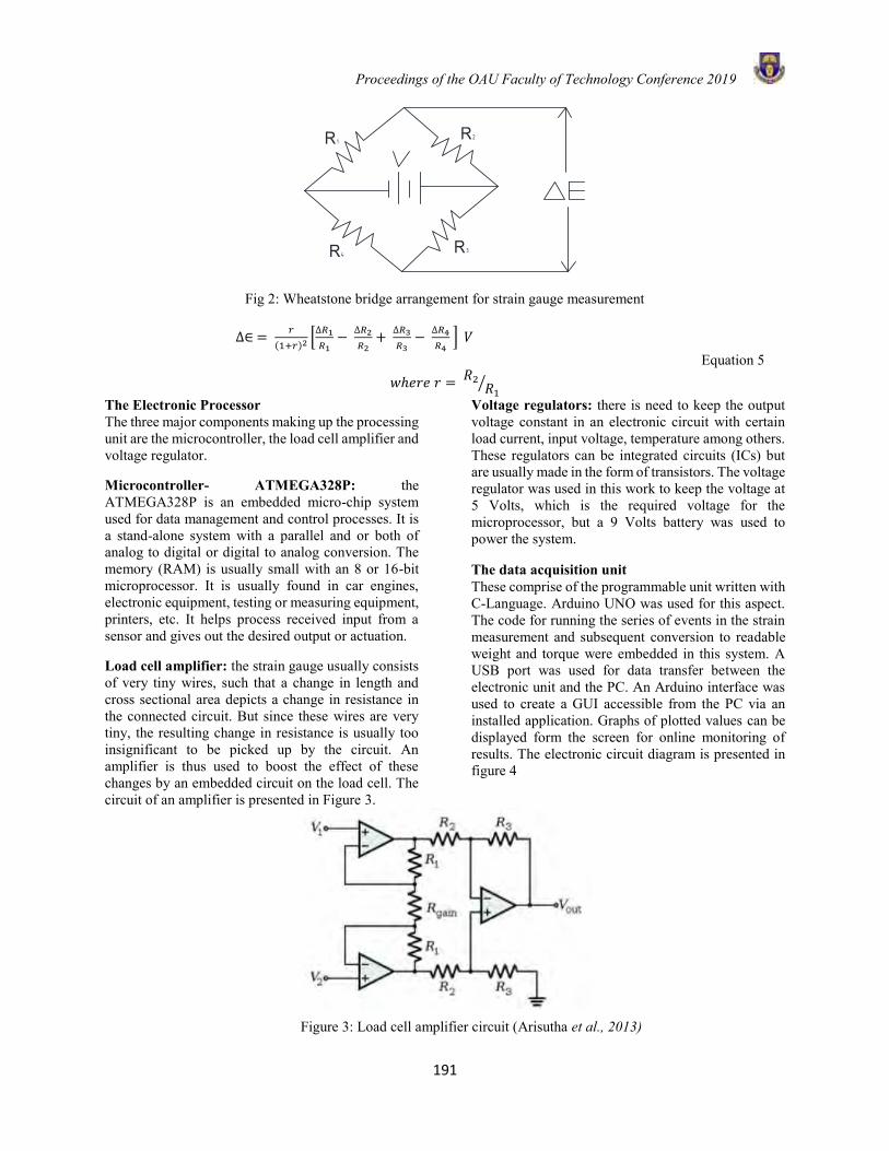
Proceedings of the OAU Faculty of Technology Conference 2019
191
R2R 1
R4R3
Fig 2: Wheatstone bridge arrangement for strain gauge measurement
∆∈ =
𝑟
(1+𝑟)2[∆𝑅1
𝑅1−
∆𝑅2
𝑅2+
∆𝑅3
𝑅3−
∆𝑅4
𝑅4 ] 𝑉
Equation 5 𝑤ℎ𝑒𝑟𝑒 𝑟 =
𝑅2𝑅1
⁄ The Electronic Processor The three major components making up the processing unit are the microcontroller, the load cell amplifier and voltage regulator. Microcontroller- ATMEGA328P: the ATMEGA328P is an embedded micro-chip system used for data management and control processes. It is a stand-alone system with a parallel and or both of analog to digital or digital to analog conversion. The memory (RAM) is usually small with an 8 or 16-bit microprocessor. It is usually found in car engines, electronic equipment, testing or measuring equipment, printers, etc. It helps process received input from a sensor and gives out the desired output or actuation. Load cell amplifier: the strain gauge usually consists of very tiny wires, such that a change in length and cross sectional area depicts a change in resistance in the connected circuit. But since these wires are very tiny, the resulting change in resistance is usually too insignificant to be picked up by the circuit. An amplifier is thus used to boost the effect of these changes by an embedded circuit on the load cell. The circuit of an amplifier is presented in Figure 3.
Voltage regulators: there is need to keep the output voltage constant in an electronic circuit with certain load current, input voltage, temperature among others. These regulators can be integrated circuits (ICs) but are usually made in the form of transistors. The voltage regulator was used in this work to keep the voltage at 5 Volts, which is the required voltage for the microprocessor, but a 9 Volts battery was used to power the system. The data acquisition unit These comprise of the programmable unit written with C-Language. Arduino UNO was used for this aspect. The code for running the series of events in the strain measurement and subsequent conversion to readable weight and torque were embedded in this system. A USB port was used for data transfer between the electronic unit and the PC. An Arduino interface was used to create a GUI accessible from the PC via an installed application. Graphs of plotted values can be displayed form the screen for online monitoring of results. The electronic circuit diagram is presented in figure 4
Figure 3: Load cell amplifier circuit (Arisutha et al., 2013)

Proceedings of the OAU Faculty of Technology Conference 2019
192
Figure 4. The circuit design of the electronic processor
Calibration Standard weights and known torques were selected for this purpose. Initial readings of the weights and torque were taken with the load cell. The graph of the standard values were plotted against the measured values. The equation of the resulting plot was determined and this was inserted into the code to make necessary output for the sensor read out. The readings of the calibrated torquemeter was taken three times to ascertain its correctness.
The Testing After the calibration process the torquemeter was used to measure the previous weights (20g, 50g, 100g, 200g, 300g, 500g, 600g, 700g, 800g, and 1000g) and the drilling machine torque. The result of the measurement was then recorded.
The percentage error was also calculated to determine the accuracy of the torquemeter.
% Error = x 100 Equation 6
The standard deviation between readings of the same quantity taken at different time were calculated thus:
𝑆. 𝐷 = √∑ (𝑥−)2𝑥=𝑗
𝑥=𝑖
𝑛−1 Equation 7
Where i= first reading j= last reading 𝑥= individual reading = mean n = no of reading
RESULTS AND DISCUSSION The strain gauge torquemeter is intended as a practical measuring instrument and its operating range is limited by the capacity of the load cell sensor used. The final outcome of the equipment is shown in Plate 1 while the display when in idle position is presented in Plate 2. The signal received by the microcontroller (ATMEGA328P) as a result of what the load cell sensed was processed and interpreted by the microcontroller. The microcontroller was connected to the alphanumeric LCD to display whatever results been processed by the microcontroller and also the microcontroller was connected with USB to TTL converter, which enable display of result on the output device such as computer in the case of multiple or instantaneous output which need to be noted or recorded during the measurement operation. The later operation was performed with the Arduino software.
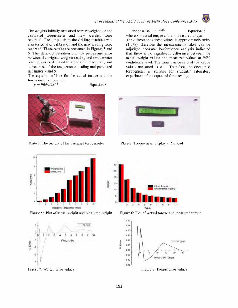
Proceedings of the OAU Faculty of Technology Conference 2019
193
The weights initially measured were reweighed on the calibrated torquemeter and new weights were recorded. The torque from the drilling machine was also tested after calibration and the new reading were recorded. These results are presented in Figures 5 and 6. The standard deviation and the percentage error between the original weights reading and torquemeter reading were calculated to ascertain the accuracy and correctness of the torquemeter reading and presented in Figures 7 and 8. The equation of line for the actual torque and the torquemeter values are;
𝑦 = 9069.2𝑥−1 Equation 8
and 𝑦 = 8411𝑥−0.988 Equation 9 where x = actual torque and y = measured torque The difference is these values is approximately unity (1.078), therefore the measurements taken can be adjudged accurate. Performance analysis indicated that there is no significant difference between the actual weight values and measured values at 95% confidence level. The same can be said of the torque values measured as well. Therefore, the developed torquemeter is suitable for students’ laboratory experiments for torque and force testing.
Plate 1: The picture of the designed torquemeter Plate 2: Torquemeter display at No load
Figure 5: Plot of actual weight and measured weight Figure 6: Plot of Actual torque and measured torque
Figure 7: Weight error values Figure 8: Torque error values
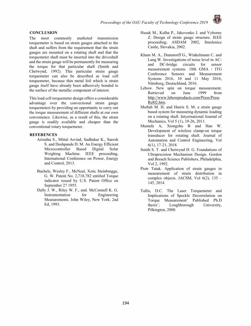
Proceedings of the OAU Faculty of Technology Conference 2019
194
CONCLUSION The most commonly marketed transmission torquemeter is based on strain gauges attached to the shaft and suffers from the requirement that the strain gauges are mounted on a rotating shaft and that the torquemeter shaft must be inserted into the driveshaft and the strain gauge will be permanently for measuring the torque for that particular shaft (Smith and Chetwynd, 1992). This particular strain gauge torquemeter can also be described as load cell torquemeter, because thin metal foil which is strain gauge itself have already been adhesively bonded to the surface of the metallic component of interest.
This load cell torquemeter design offers a considerable advantage over the convectional strain gauge torquemeters by providing an opportunity to carry out the torque measurement of different shafts at our own convenience. Likewise, as a result of this, the strain gauge is readily available and cheaper than the conventional rotary torquemeter.
REFERENCES Arisutha S., Mittal Arvind, Sudhakar K., Suresh
S. and Deshpande D. M. An Energy Efficient Microcontroller Based Digital Solar Weighing Machine. IEEE proceeding, International Conference on Power, Energy and Control, 2013.
Buchele, Wesley F., McNeal, Xzin; Steinbmgge, G. W. Patent No. 2,718,782 entitled Torque indicator issued by U.S. Patent Office on September 27 1955.
Dally J. W., Riley W. F., and. McConnell K. G. Instrumentation for Engineering Measurements. John Wiley, New York. 2nd Ed, 1993.
Husak M., Kulha P., Jakovenko J. and Vyborny Z. Design of strain gauge structure. IEEE proceeding; ASDAM 2002, Smolenice Castle, Slovakia, 2002.
Kham M. A., Dumstorff G., Winkelmann C. and Lang W. Investigations of noise level in AC-and DC-bridge circuits for sensor measurement systems. 18th GMA / ITG Conference Sensors and Measurement Systems 2016, 10 and 11 May 2016, Nürnberg, Deutschland, 2016.
Lebow. New spin on torque measurement. Retrieved on June 1999 from http://www.lebowproducts.com/Press/PressRel02.htm.
Muftah M. H. and Harris S. M. a strain gauge based system for measuring dynamic loading on a rotating shaft. Intyernational Journal of Mechanics, Vol 5 (1), 19-26, 2011.
Mustafa A, Xiongzhu B and Han W. Development of wireless clamp-on torque transducer for rotating shaft. Journal of Automation and Control Engineering, Vol 6(1), 17-21, 2018.
Smith S. T. and Chetwynd D. G. Foundations of Ultraprecision Mechanism Design. Gordon and Breach Science Publishers, Philadelphia, Vol 2, 1992.
Piotr Tutak. Application of strain gauges in measurement of strain distribution in complex objects. JACSM, Vol 6(2), 135 – 145, 2014.
Tullis, D.C. The Laser Torquemeter and Implications of Speckle Decorrelation on Torque Measurement’ Published Ph.D thesis’; Loughborough University, Pilkington, 2000.
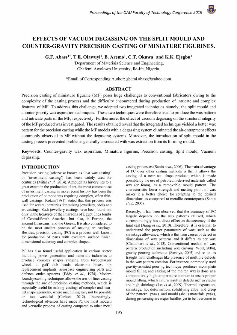
Proceedings of the OAU Faculty of Technology Conference 2019
195
EFFECTS OF VACUUM DEGASSING ON THE SPLIT MOULD AND COUNTER-GRAVITY PRECISION CASTING OF MINIATURE FIGURINES.
G.F. Abass1*, T.E. Olawuyi1, B. Aremo1, C.T. Okuwa1 and K.K. Ejegbu1 1Department of Materials Science and Engineering,
Obafemi Awolowo University, Ile-Ife, Nigeria.
*Email of Corresponding Author: [email protected]
ABSTRACT Precision casting of miniature figurine (MF) poses huge challenges to conventional fabricators owing to the complexity of the casting process and the difficulty encountered during production of intricate and complex features of MF. To address this challenge, we adapted two integrated techniques namely, the split mould and counter-gravity wax aspiration techniques. These two techniques were therefore used to produce the wax pattern and intricate parts of the MF, respectively. Furthermore, the effect of vacuum degassing on the structural integrity of the MF produced was investigated. The results obtained reveal that the integrated technique yielded a better wax pattern for the precision casting while the MF models with a degassing system eliminated the air-entrapment effects commonly observed in MF without the degassing systems. Moreover, the introduction of split mould in the casting process prevented problems generally associated with wax extraction from its forming mould.
Keywords: Counter-gravity wax aspiration, Miniature figurine, Precision casting, Split mould, Vacuum degassing.
INTRODUCTION Precision casting (otherwise known as ‘lost wax casting’ or ‘investment casting’) has been widely used for centuries (Mital et al., 2014). Although its history lies to a great extent in the production of art, the most common use of investment casting in more recent history has been the production of components requiring complex, often thin-wall castings. Kotzin(1981) stated that this process was used for several centuries for making jewellery, idols and art castings. Such jewellery castings have been found not only in the treasures of the Pharaohs of Egypt, Inca tombs of Central/South America, but also, in Europe, the ancient Etruscans, and the Greeks. It is also considered to be the most ancient process of making art castings. Besides, precision casting (PC) is a process well known for production of parts with excellent surface finish, dimensional accuracy and complex shapes. PC has also found useful application in various sector including power generation and materials industries to produce complex shapes ranging from turbocharger wheels to golf club heads, electronic boxes, hip replacement implants, aerospace engineering parts and defence outlet systems (Eddy et al., 1974). Modern foundry/casting techniques allows the use of finer casting through the use of precision casting methods, which is especially useful for making castings of complex and near-net shape geometry, where machining may not be possible or too wasteful (Carlton, 2012). Interestingly, technological advances have made PC the most modern and versatile process of casting compared to other metal
casting processes (Sanin et al., 2006). The main advantage of PC over other casting methods is that it allows the casting of a near net- shape product, which is made possible by the use of petroleum-derived materials called wax (or foam), as a removable mould pattern. The characteristic lower strength and melting point of wax makes it a better choice for sculpting to the desired dimensions as compared to metallic counterparts (Sanin et al., 2006). Recently, it has been observed that the accuracy of PC largely depends on the wax patterns utilized, which correspondingly has a direct effect on the accuracy of the final cast (Jiang et al., 2010). Therefore, it is essential to understand the proper parameters of wax, such as the shrinkage allowance, which is the main causes of defect in dimensions of wax patterns and it differs as per wax (Chaudhari et al., 2013). Conventional method of wax pattern production including wax carving (Wolf, 2004), gravity pouring technique (Saraiya, 2003) and so on, is fraught with challenges like presence of multiple defects in the wax pattern creation. For instance, commonly used gravity-assisted pouring technique produces incomplete mould filling and casting of the molten wax is done at a comparatively high temperature in order to ensure proper mould filling, which in turn result in defects such as cracks and high shrinkage (Lee et al., 2009). Thermal expansion, shrinkage, hot deformation, solidifying alloy, and creep of the pattern (wax) and mould (shell) materials (wax), during processing are major hurdles yet to be overcome in
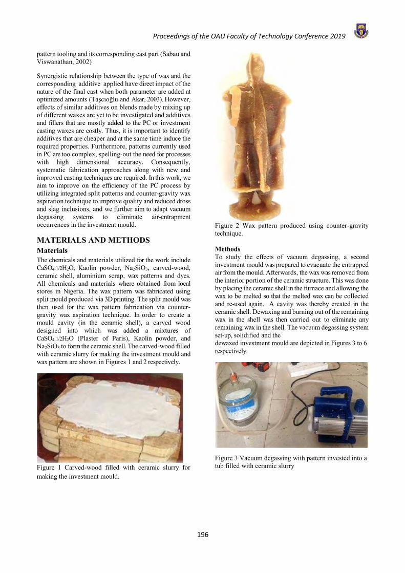
Proceedings of the OAU Faculty of Technology Conference 2019
196
pattern tooling and its corresponding cast part (Sabau and Viswanathan, 2002) Synergistic relationship between the type of wax and the corresponding additive applied have direct impact of the nature of the final cast when both parameter are added at optimized amounts (Taşcıoğlu and Akar, 2003). However, effects of similar additives on blends made by mixing up of different waxes are yet to be investigated and additives and fillers that are mostly added to the PC or investment casting waxes are costly. Thus, it is important to identify additives that are cheaper and at the same time induce the required properties. Furthermore, patterns currently used in PC are too complex, spelling-out the need for processes with high dimensional accuracy. Consequently, systematic fabrication approaches along with new and improved casting techniques are required. In this work, we aim to improve on the efficiency of the PC process by utilizing integrated split patterns and counter-gravity wax aspiration technique to improve quality and reduced dross and slag inclusions, and we further aim to adapt vacuum degassing systems to eliminate air-entrapment occurrences in the investment mould.
MATERIALS AND METHODS Materials The chemicals and materials utilized for the work include CaSO4.1/2H2O, Kaolin powder, Na2SiO3, carved-wood, ceramic shell, aluminium scrap, wax patterns and dyes. All chemicals and materials where obtained from local stores in Nigeria. The wax pattern was fabricated using split mould produced via 3D printing. The split mould was then used for the wax pattern fabrication via counter-gravity wax aspiration technique. In order to create a mould cavity (in the ceramic shell), a carved wood designed into which was added a mixtures of CaSO4.1/2H2O (Plaster of Paris), Kaolin powder, and Na2SiO3 to form the ceramic shell. The carved-wood filled with ceramic slurry for making the investment mould and wax pattern are shown in Figures 1 and 2 respectively.
Figure 1 Carved-wood filled with ceramic slurry for making the investment mould.
Figure 2 Wax pattern produced using counter-gravity technique. Methods To study the effects of vacuum degassing, a second investment mould was prepared to evacuate the entrapped air from the mould. Afterwards, the wax was removed from the interior portion of the ceramic structure. This was done by placing the ceramic shell in the furnace and allowing the wax to be melted so that the melted wax can be collected and re-used again. A cavity was thereby created in the ceramic shell. Dewaxing and burning out of the remaining wax in the shell was then carried out to eliminate any remaining wax in the shell. The vacuum degassing system set-up, solidified and the dewaxed investment mould are depicted in Figures 3 to 6 respectively.
Figure 3 Vacuum degassing with pattern invested into a tub filled with ceramic slurry
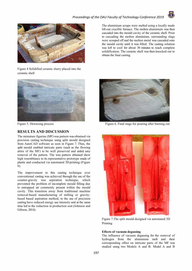
Proceedings of the OAU Faculty of Technology Conference 2019
197
Figure 4 Solidified ceramic slurry placed into the ceramic shell
The aluminium scraps were melted using a locally made lift-out crucible furnace. The molten aluminium was then cascaded into the mould cavity of the ceramic shell. Prior to cascading the molten aluminium, surrounding slags were scooped off and the molten metal was cascaded onto the mould cavity until it was filled. The casting solution was left to cool for about 30 minutes to reach complete solidification. The ceramic shell was then knocked out to obtain the final casting.
Figure 5. Dewaxing process Figure 6. Final stage for pouring after burning out RESULTS AND DISCUSSION The miniature figurine (MF) wax pattern was obtained via precision casting technique using split mould designed from AutoCAD software as seen in Figure 7. Thus, the split mould enabled intricate parts (such as the flowing attire of the MF) to be well preserved and aided easy removal of the pattern. The wax pattern obtained show high resemblance to its representative prototype made of plastic and conducted via automated 3D printing (Figure 8). The improvement to this casting technique over conventional casting was achieved through the use of the counter-gravity wax aspiration technique, which prevented the problem of incomplete mould filling due to entrapped air commonly present within the mould cavity. This transition away from traditional machine removal-based manufacturing of milling or gravity-based based aspiration method, to the use of precision casting have reduced energy use intensity and at the same time led to the reduction in production cost (Johnson and Gibson, 2014).
Figure 7.The split mould designed via automated 3D Printing Effects of vacuum degassing The influence of vacuum degassing for the removal of hydrogen from the aluminium melt and their corresponding effect on intricate parts of the MF was studied using two Models A and B. Model A and B
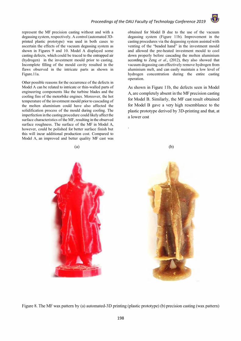
Proceedings of the OAU Faculty of Technology Conference 2019
198
represent the MF precision casting without and with a degassing system, respectively. A control (automated 3D-printed plastic prototype) was used in both cases to ascertain the effects of the vacuum degassing system as shown in Figures 9 and 10. Model A displayed some casting defects, which could be traced to the entrapped air (hydrogen) in the investment mould prior to casting. Incomplete filling of the mould cavity resulted in the flaws observed in the intricate parts as shown in Figure.11a. Other possible reasons for the occurrence of the defects in Model A can be related to intricate or thin-walled parts of engineering components like the turbine blades and the cooling fins of the motorbike engines. Moreover, the hot temperature of the investment mould prior to cascading of the molten aluminium could have also affected the solidification process of the mould during cooling. The imperfection in the casting procedure could likely affect the surface characteristics of the MF, resulting in the observed surface roughness. The surface of the MF in Model A, however, could be polished for better surface finish but this will incur additional production cost. Compared to Model A, an improved and better quality MF cast was
obtained for Model B due to the use of the vacuum degassing system (Figure 11b). Improvement in the casting procedures via the degassing system assisted with venting of the “beaded hand” in the investment mould and allowed the pre-heated investment mould to cool down properly before cascading the molten aluminium according to Zeng et al., (2012), they also showed that vacuum degassing can effectively remove hydrogen from aluminium melt, and can easily maintain a low level of hydrogen concentration during the entire casting operation. As shown in Figure 11b, the defects seen in Model A, are completely absent in the MF precision casting for Model B. Similarly, the MF cast result obtained for Model B gave a very high resemblance to the plastic prototype derived by 3D-printing and that, at a lower cost
.
(a)
(b)
Figure 8. The MF wax pattern by (a) automated-3D printing (plastic prototype) (b) precision casting (wax pattern)

Proceedings of the OAU Faculty of Technology Conference 2019
199
(a) (b)
Figure 9 Comparison between (a) MF from 3D-printing (plastic prototype) (b) MF cast for Model A without vacuum degassing.
(a) (b)
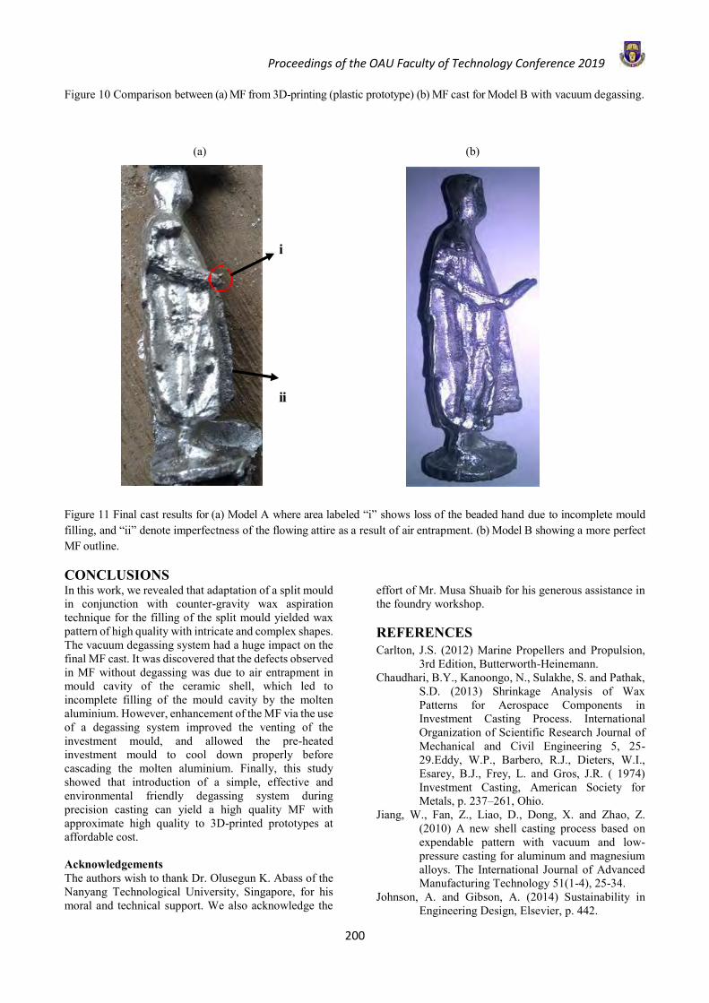
Proceedings of the OAU Faculty of Technology Conference 2019
200
Figure 10 Comparison between (a) MF from 3D-printing (plastic prototype) (b) MF cast for Model B with vacuum degassing.
(a) (b)
i
ii
Figure 11 Final cast results for (a) Model A where area labeled “i” shows loss of the beaded hand due to incomplete mould filling, and “ii” denote imperfectness of the flowing attire as a result of air entrapment. (b) Model B showing a more perfect MF outline.
CONCLUSIONS In this work, we revealed that adaptation of a split mould in conjunction with counter-gravity wax aspiration technique for the filling of the split mould yielded wax pattern of high quality with intricate and complex shapes. The vacuum degassing system had a huge impact on the final MF cast. It was discovered that the defects observed in MF without degassing was due to air entrapment in mould cavity of the ceramic shell, which led to incomplete filling of the mould cavity by the molten aluminium. However, enhancement of the MF via the use of a degassing system improved the venting of the investment mould, and allowed the pre-heated investment mould to cool down properly before cascading the molten aluminium. Finally, this study showed that introduction of a simple, effective and environmental friendly degassing system during precision casting can yield a high quality MF with approximate high quality to 3D-printed prototypes at affordable cost. Acknowledgements The authors wish to thank Dr. Olusegun K. Abass of the Nanyang Technological University, Singapore, for his moral and technical support. We also acknowledge the
effort of Mr. Musa Shuaib for his generous assistance in the foundry workshop. REFERENCES Carlton, J.S. (2012) Marine Propellers and Propulsion,
3rd Edition, Butterworth-Heinemann. Chaudhari, B.Y., Kanoongo, N., Sulakhe, S. and Pathak,
S.D. (2013) Shrinkage Analysis of Wax Patterns for Aerospace Components in Investment Casting Process. International Organization of Scientific Research Journal of Mechanical and Civil Engineering 5, 25-29.Eddy, W.P., Barbero, R.J., Dieters, W.I., Esarey, B.J., Frey, L. and Gros, J.R. ( 1974) Investment Casting, American Society for Metals, p. 237–261, Ohio.
Jiang, W., Fan, Z., Liao, D., Dong, X. and Zhao, Z. (2010) A new shell casting process based on expendable pattern with vacuum and low-pressure casting for aluminum and magnesium alloys. The International Journal of Advanced Manufacturing Technology 51(1-4), 25-34.
Johnson, A. and Gibson, A. (2014) Sustainability in Engineering Design, Elsevier, p. 442.

Proceedings of the OAU Faculty of Technology Conference 2019
201
Kotzin, E.L. (1981) Metal Casting and Moulding Processes, American Foundrymen Society Inc., Illinois, USA.
Mital, A., Desai, A., Subramanian, A. and Mital, A. (2014) A Structured Approach to Consumer Product Development, Design, and Manufacture, Second Edition, Product Development, Elsevier.
Sabau, A.S. and Viswanathan, S. (2002) Prediction of Wax Pattern Dimensions in Investment Casting. Transactions-American Foundrymen Society 1, 733-746.
Sanin, V., Yukhvid, V., Sytschev, A. and Andreev, D. (2006) Combustion synthesis of cast intermetallic Ti-Al-Nb alloys in a centrifugal machine. Kovove Material 44, 49–55.
Saraiya, R.D. (2003) Understanding Investment Casting Waxes-Pattern Making, Allied Publishers Private Limited, New Delhi, India, pp.113-114.
Taşcıoğlu, S. and Akar, N. (2003) Conversion of an Investment Casting Sprue Wax to a Pattern Wax by Chemical Agents. Materials and Manufacturing Processes 18(5),753-768.
Wolf, K. (2004) Ganoskin Jewelry Making Resources, Cut Loose-Wax Carving Basics Part 1, Manufacturing Jewelers and Suppliers of America, https://www.Ganoskin.Com/Article/Cut-Loose-Wax-Carving-Basics-Parrt-1/. Accessed: 12th January, 2018.
Zeng, J., Gu, P. and Wang, Y. (2012) Investigation of Inner Vacuum Sucking method for degassing of molten aluminum. Materials Science and Engineering: B 177(19), 1717-1720.
Proceedings of the OAU Faculty of Technology Conference 2019
202
ENGINEERING ECONOMY STUDIES ON DEVELOPMENT AND PRODUCTION OF SPORTS DRINK FROM INDIGENOUS FRUITS
A. B. Ilori1,*, B. O. Oyedoyin2, O. B. Oluwole3, T. E. Akinwale4 and O. V. Oke5 *1,2Department of Planning Technology Transfer and Information Management
3,4,5Department of Food Technology Federal Institute of Industrial Research, Oshodi (FIIRO) Lagos.
*Corresponding Author E-Mail: [email protected]
ABSTRACT This study determined the economic viability of the industrial production of sports drink developed at FIIRO laboratory from indigenous fruits.Based on an output of 50 x 106litres/year, and the yield of the products, the quantities and costs of the raw materials, date fruit, watermelon, glucose, sodium chloride, ascorbic acid and sodium metabisulphiteusing their market prices, were estimated at 100% capacity utilizations (CU). The costs of land acquisition and factory building were obtained from contractors. The labour cost was also estimated for 120 staffs. The selling price ₦250/litre of a similar product was adopted. Annual worth (AW) and present worth (PW) were calculated and used to establish the profitability of the products. The results showed that the proposed plant would produce 50 x 106 units of each of the sports drink at full CU. The PW and AW showed that all the products were economically viable with PW and AW greater than zero at 100% CU. At 100%, all the profitability indices for the products were positive. In conclusion, production of sports drinks using indigenous fruits is technologically and economically viable. Keywords: Economic, date fruit, watermelon and production INTRODUCTION Susan (2003) opined that sports drinks are different things to different people. Sports drink is a drink consumed either in preparation for exercise, during exerciseitself or as a recovery drink after exercise. A drink is a liquid substance and as such, water isa main ingredient(Susan, 2003). However, in a sports drink a variety of nutrientsand other substances will be dissolved in the water to make thefinal consumed product.Sport drink is a beverage designed to help athletes rehydrate, as well as replenish electrolytes and sugars that are lost or depleted after exercise, training or competition (Berninget al., 1998; Mettleret al.,2006; Vaibhavi and Bhakti, 2014). The main role of sports drinks is probably,therefore, to provide a large amount of water in addition toother components which could otherwise be obtained from food. However, there is currently no sport drink produced from indigenous fruits in Nigeria despite our national and international prominence in sports such as nation’s cup, world cup and Olympics among others. Production of sport drinks from our local raw materials will bring enormous benefits for the country. Post-harvest losses of indigenous fruits in Nigeria is about 15% (FAOSTAT, 2017), this loss could be reduced with the production of isotonic sport drink using indigenous fruits. Recently, the technology for the sport drinks production has been established at the Federal Institute of Industrial Research, Oshodi, Lagos state. The physiological test have been carried out on toad to determine the effect of the sport drink on strain of contraction, duration of muscle contraction and load and work done by the
muscle. The raw materials include date fruit, watermelon and other ingredients. According to Anjiliet al., (2015) date palm (Phoenix dactyliferaL.) is a palm in the genus Phoenix, cultivated for its edible sweet fruit. Dates are widely distributed and facilitated by the fact that dates have high calorie food, with a long-keeping quality (FAO, 2012). Date fruit also can be made into juice, vinegar, wine, beer, sugar, syrup, honey, chutney, pickle, paste, dip, and food flavoring (Barreveld, 1993 and Glasneret al., 2002). It is an ideal food for people of different ages, providing the most important essential nutrients such as protein, fiber, carbohydrates, fat and minerals (Al-Farsi et al., 2005 and Vyawahareet al., 2009). It has also been considered a complete diet and a very important item of food. It has plenty of vitamins and minerals, 25% more potassium than bananas free of fat, sodium and cholesterol. Date plays an important role in the diet and treatment of obesity. It is also the most important source of energy and food in date producing and non date producing areas (Foroogh, 2009). Al-Shahib and Marshall (2003a) posited that worldwide production of date fruit has increasedalmost threefold over the last 40 years, reaching 7.68 million tons in 2010. Dates fruits are loaded with various nutrients withmedicinal importance for ailment of certain diseases. As a result of its high nutritional value and its long life the date palm hasbeen mentioned as the ‘tree of life’ (Augstburger, et al., 2002).Whole part of date fruits is useful, also the by-products arising from date processing are used for different purposes. Date fruits are also used in the preparationof sweets, snacks,
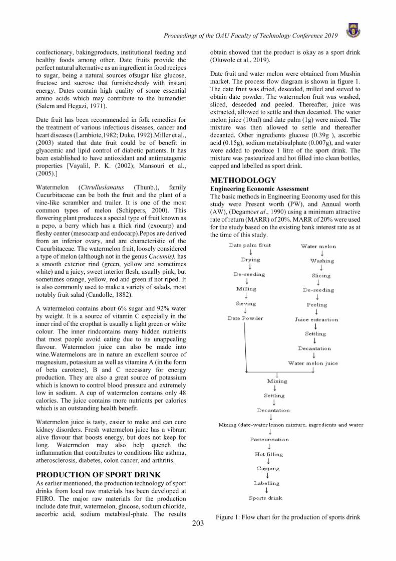
Proceedings of the OAU Faculty of Technology Conference 2019
203
confectionary, bakingproducts, institutional feeding and healthy foods among other. Date fruits provide the perfect natural alternative as an ingredient in food recipes to sugar, being a natural sources ofsugar like glucose, fructose and sucrose that furnishesbody with instant energy. Dates contain high quality of some essential amino acids which may contribute to the humandiet (Salem and Hegazi, 1971). Date fruit has been recommended in folk remedies for the treatment of various infectious diseases, cancer and heart diseases (Lambiote,1982; Duke, 1992).Miller et al., (2003) stated that date fruit could be of benefit in glyacemic and lipid control of diabetic patients. It has been established to have antioxidant and antimutagenic properties [Vayalil, P. K. (2002); Mansouri et al., (2005).] Watermelon (Citrulluslanatus (Thunb.), family Cucurbitaceae can be both the fruit and the plant of a vine-like scrambler and trailer. It is one of the most common types of melon (Schippers, 2000). This flowering plant produces a special type of fruit known as a pepo, a berry which has a thick rind (exocarp) and fleshy center (mesocarp and endocarp).Pepos are derived from an inferior ovary, and are characteristic of the Cucurbitaceae. The watermelon fruit, loosely considered a type of melon (although not in the genus Cucumis), has a smooth exterior rind (green, yellow and sometimes white) and a juicy, sweet interior flesh, usually pink, but sometimes orange, yellow, red and green if not riped. It is also commonly used to make a variety of salads, most notably fruit salad (Candolle, 1882). A watermelon contains about 6% sugar and 92% water by weight. It is a source of vitamin C especially in the inner rind of the cropthat is usually a light green or white colour. The inner rindcontains many hidden nutrients that most people avoid eating due to its unappealing flavour. Watermelon juice can also be made into wine.Watermelons are in nature an excellent source of magnesium, potassium as well as vitamins A (in the form of beta carotene), B and C necessary for energy production. They are also a great source of potassium which is known to control blood pressure and extremely low in sodium. A cup of watermelon contains only 48 calories. The juice contains more nutrients per calories which is an outstanding health benefit. Watermelon juice is tasty, easier to make and can cure kidney disorders. Fresh watermelon juice has a vibrant alive flavour that boosts energy, but does not keep for long. Watermelon may also help quench the inflammation that contributes to conditions like asthma, atherosclerosis, diabetes, colon cancer, and arthritis. PRODUCTION OF SPORT DRINK As earlier mentioned, the production technology of sport drinks from local raw materials has been developed at FIIRO. The major raw materials for the production include date fruit, watermelon, glucose, sodium chloride, ascorbic acid, sodium metabisul-phate. The results
obtain showed that the product is okay as a sport drink (Oluwole et al., 2019). Date fruit and water melon were obtained from Mushin market. The process flow diagram is shown in figure 1. The date fruit was dried, deseeded, milled and sieved to obtain date powder. The watermelon fruit was washed, sliced, deseeded and peeled. Thereafter, juice was extracted, allowed to settle and then decanted. The water melon juice (10ml) and date palm (1g) were mixed. The mixture was then allowed to settle and thereafter decanted. Other ingredients glucose (0.39g ), ascorbic acid (0.15g), sodium metabisulphate (0.007g), and water were added to produce 1 litre of the sport drink. The mixture was pasteurized and hot filled into clean bottles, capped and labelled as sport drink. METHODOLOGY Engineering Economic Assessment The basic methods in Engineering Economy used for this study were Present worth (PW), and Annual worth (AW), (Degamoet al., 1990) using a minimum attractive rate of return (MARR) of 20%. MARR of 20% were used for the study based on the existing bank interest rate as at the time of this study.
Figure 1: Flow chart for the production of sports drink

Proceedings of the OAU Faculty of Technology Conference 2019
204
Present worth (PW): The present worth (PW) method is based on the concept of all cash flows relative to some base or beginning point in time called the present. That is all cash inflows and outflows are discounted to the base point at a minimum attractive rate of return (MARR) (Degamoet al., 1990).
=
=
=
=
−=kn
n
kn
nki NiAPENiAPRPW
1 1)%,.,./(.).%.,./( -
I(A/P, i%, N) + St (P/F, i%, N) (1) Where
Ri = future cash inflows at the end of each year or a period
Eĸ = future cash outflow at the end of each year S is Salvage value at period k A is annual amount i is the MARR P is present amount N is study period or life (years) of the project F is future amount I is Investment cost Annual worth (AW): is a uniform annual series of amounts, for a stated study period that is equivalent to cash inflows (receipts or savings) and/or cash outflows (expenses) under consideration. In other words, the annual worth of a project is its annual equivalent receipts (or savings) (R) minus annual equivalent expenses (E), less its annual equivalent capital recovery (CR) amount which is defined below. An annual equivalent value of R, E, and CR is computed as the MARR. The study period is denoted by N, which is usually years. In equation form, the annual worth is AW = R – E – CR (2) CR = I (A/P, i%, N) – S(A/F, i%, N) (3) Where R = annual equivalent receipt E = annual equivalent expenses CR = annual equivalent capital recovery The project is worthwhile if AW > 0. (DeGarmo et al., 1990). As long as the annual worth is greater than or equal to zero, the project is economically attractive; otherwise, it is not. Engineering Economic Analysis Investment costs The investment cost which is usually referred to as first cost (Degarmo et al., 1990) is made up of costs of land, building and equipment/machinery acquisition. It also includes costs of utilities and working capital. The cost of the plant/machinery was obtained from an industry in Lagos while the costs of land, factory building utilities were obtained from professionals (surveyors and estate managers) in the fields. The working capital was estimated as 10% of the cost of the plant. Operating and Maintenance Cost The raw material estimates was based on (i) the output of 50 million litres per year of the plant at
100% capacity utilization.
(ii) the market prices, the costs of raw materials for the products were then estimated.
Labour and other operating costs were estimated based on what obtains currently in a similar organization. The salvage value (Sĸ) for period k was assumed to be the book value (BVĸ) of the asset at period (k). The straight line depreciation method was used for the study. It was assumed that the loss in value is directly proportional to the age of the asset (Degarmo et al., 1990). Thus depreciation BVĸ was calculated thus:
dĸ = B – S (4) N
Dĸ = K (B - S) (5) N
BVĸ ≡ B – Dĸ ≡ Sĸ (6) Where: N = the depreciable life of the asset B = cost of the machinery/equipment dĸ = annual depreciation deduction in the kth year 1 ≤ K ≤ N S = salvage value at the end of the depreciation life of
the asset Dĸ = cumulative depreciation through year k The standard cost per litre of production of the sport drink was calculated (De Garmo, 1990). The selling price of a similar product (N250/litre) in the market was used to estimate the revenue from sales of the drink. RESULT AND DISCUSSION Engineering Economic Analysis Based on an output of 50,000x106litres/year, and the yield of the products, the quantities and costs of the raw materials, costs of the raw materials (date fruit, watermelon, glucose, sodium chloride, ascorbic acid, sodium metabisulphite and ascorbic acid) using their market prices, were estimated at 100% capacity utilizations (CU). Table 1 shows the first cost to be (N1,161,265.1x103)which comprises of costs of land and building (N55,000 x103), plant and machineries (N1,047,171.1x103), auxiliary equipment (N1,500x103) utility equipment (N11,900x103), furniture and fittings (N5,500 x103), motor vehicles (N29,000x103) and working capital (N11,984x103). The data for engineering economic analysis such as investment cost, annual disbursement and revenue are shown in Tables 2. The Product has the investment cost of N1,161,265.1x103. The investment cost includes costs of equipment acquisition, land and building, motor vehicles and working capital (Table 1). The annual disbursements vary with product type. These annual disbursements include the cost ofraw materials, labour cost, energy cost, operating and maintenance cost and insurance cost. The operating and maintenance cost include costs of maintenance of machinery and factory building, office

Proceedings of the OAU Faculty of Technology Conference 2019
205
running, transportation and travels, telephone and auditing and other professional fees. The utility costs are the costs of electricity, fuel, diesel, lubricants and other consumables. The factory would require a general manager, secretary, production manager, accountant and
engineer. Other workers include, among others, professionals and factory labourers. The annual cost estimate for labour is N48,600x103 at 100% capacity utilization (Table 2).
Table 1 Land and machinery acquisition for the production of sports drink using indigenous fruits
Description of Item
Number of Units
Unit Cost x 103
Amount (N:k) x 103
Sub-Total (N:k) x 103
(A) Land and Building (i) 5 hectare of land 5 1000 5000
(ii) Factory Building - - 50,000 Sub-Total - - 55,000 55,000
(B) Plant and Machineries (i) Raw materials processing plant 50million @
N250 -
950,000
(ii) Tetrapak packaging plant
(iii) (iv)
Fruit washing machine Contingencies 10% of imported new equipment
1 -
2,171.1 -
2,171.1 95,000
Sub-Total 1,047,171.1 (C) Auxiliary Equipment
(i) Storage tanks 7 90 630 (ii) Wheel barrows 4 20 80
Sub-Total 710 710 (D) Utility Equipment
(i) Generating Set 200KVA 1 10,000 10,000 (ii) Bore hole 1 650 650
(iii) Electric pump 5 - 1,250 Sub-Total 11,900 11,900
(E) Furniture and Fittings (i) Office tables and chairs - - 2,500
(ii) ACs, fans. - - 3,000 Sub-Total - - 5,500 5,500
(F) Motor Vehicles (i) Delivery Van 2 4,000 8,000
(ii) Pick up Hilux 1 11,000 11,000 (iii) Trucks 2 5,000 10,000
Sub-Total 29,000 29,000 (H) Working Capital
Total - - 11,984 11,984
1,161,265.1
Table 2. Cash Flow of Industrial Production Sports drink using indigenous fruits S/No. Description of Item Amount (N) x103
A. Investment (i) Land and Building 55,000 (ii) Plant and Machinery 1,047,171.1 (iii)
(iv) (v) (vi) (vii)
Auxiliary Equipment Utility Equipment Furniture and Fittings Motor Vehicles Working Capital
710 11,900 5,500
29,000 11,984
Sub-Total 1,161,265.1 B. Annual Disbursement (i)
(ii) Raw materials Labour cost
239,680 48,600
(ii) Energy cost 2,800 (iii) Maintenance cost 15,000 (iv) Insurance cost 114,376.11 Sub-Total 420,436.11
C. Revenue (i)
(ii) Sales of sport drinks (at ₦250/unit) Salvage value Sub – Total
12,500,000 5,000
12,505,000 D. MARR = 20% E. Life of the project = 20 years F. Profitability Index (i) Present Worth (PW) 59,733,082.9 (ii) Amount Worth (AW) 181,912.26
Proceedings of the OAU Faculty of Technology Conference 2019
206
The results showed that the proposed plant would produce 50 million units of each of the sport drinks at full CU. The PW (N59,733,082.9x103) and AW (N181,912.26x103) showed that all the products were economically viable with PW and AW greater than zero at 100% CU. At 100%, all the profitability indices for the products were positive. Production of sports drink using indigenous fruits is therefore technologically and economically viable.
SUMMARY AND CONCLUSION This study assesses the economic viability of the production of sports drink using indigenous fruits. The quantity of raw materials and equipment for the production of the sports drinks using indigenous fruits at industrial level were estimated and the economic viability of the products was determined. The PW and AW for the sport drinks production using indigenous fruits at 100% capacity utilization justified investment in the sports drink production. In conclusion, the development and production of sports drink from indigenous fruits is a good formulation to meet the needs of many athletes or sportsmen in many different situations. It is technologically and economically viable and consumer acceptability should not pose a serious problem. Hence, the production technology is recommended for commercialization to create wealth for people.
REFERENCES Al-Farsi, M., Alasalvar, C., Morris, A., Baron, M. and
Shahidi, F. “Comparison of Antioxidant Activity, Anthocyanins, Carotenoids, and Phenolics of three Native Fresh and Sun-dried Date (Phoenix dactylifera L.) Varieties Grown in Oman,” Journal of Agricultural and Food Chemistry, 53(19): 7592–7599, 2005.
Al-Shahib, W. and Marshall, R. J. The fruit of the datepalm: it’s possible use as the best Emir. J. Food Agric. 2012. 24(5): 371-385 http://ejfa. info/383 food for the future. Int. J. Food Sci. Nutr. 54:247-259, 2003a.
Al-Shahib, W. and Marshall, R. J.. Fatty acid content of the seeds from 14 varieties of date palm Phoenix dactylifera L. Int. J. Food Sci. Tech. 38:709-712, 2003b.
Anjili S. M., Channya F. K., Chimbekujwo I. B. Fungi Associated with Post-harvest Spoilage of Date Palm (Phoenix dactylifera L.), 2015.
Augstburger, F., Berger,J., CenskowskyU., Heid, P. Milz, J. and StreitC. Date Palm. Naturland. Germany. International Journal of Research in Agriculture and Forestry 2(11):14-22, 2002.
Barreveld, W. H. Date Palm Products (Food and Agriculture Organization of the United Nations, Agricultural Services Bulletin no. 101, Food and Agriculture Organization of the United Nations, Rome, Italy), 1993.
Candolle: Origin of Cultivated Plants, pp. 262 ff, S.U., “Water-Melon”, 1882.
Duke J.A. Handbook of Phyto-chemicals of GRAS Herbs and Other Economic Plants. Boca Raton FL: CRC Press, 1992.
FAO, Plant Production and Protection Paper No. 35. Date Production and Protection. FAO. Rome, 198-294, 2012.
FAOSTAT. Food and Agriculture Organization of the United Nations. Retrieved March 21, 2017, from http://www.fao.org/faostat/en/#data/QC, 2017.
Foroogh, B. Assessment of Antioxidant potential of date (phoenix dactylifera) fruits from Iran. (M.Sc Dissertation, University of Sains, Malaysia). 4-18, 2009.
Glasner, B., Botes, A., Zaid, A. and Emmens, J. In Date Palm Cultivation, Date Harvesting, Packing-house Management and Marketing Aspects, ed Zaid A. (Food and Agriculture Organization Plant Production and Protection paper no. 156. Food and Agriculture Organization of the United Nations, Rome, Italy), 177–208, 2002.
Ilori, A.B., Oluwale B.A. and Akanbi C.T. Engineering Economy studies on the Production of Tomato-based fruits Pulp Mixes. Journal of Industrial Research & Technology 4(1):117-130, 2015.
Salem and Hegazi Salem. S. A.and Hegazi. S.M. Chemical composition of the Egiptian dry dates, Journal of the science of Food and Agriculture. 22: 632-633, 1971.
Lambiote B. Some aspects of the role of dates in human nutrition. In: Proceedings of the First inter-national Symposium on Date Palm. Saudi Arabia: King Faisal University, 1982.
Mansouri A., Embarek G., Kokkalou E. and Kefalas P. Phenolic profile and antioxidant activity of the Algerian ripe date palm fruit (Phoenix dactyle-fera). Food Chemistry 89: 411–420, 2005.
Miller C.J., Dunn E.V. and Hashim I.B. The glycaemic index of dates/yoghurt mixed meals. Are dates ‘the candy that grows on tress’? European Journal of Clinical Nutrition 57: 247–430, 2003.
Oluwole O. B., Akinwale T.E.and Oke O.V. Development and Production of Sports Drink from Indigenous Fruits. FIIRO Unpublished Research Report, 2019.
Schippers R.R. African Indigenous Vegetable. pp. 56-60. An Overview of the Cultivated species. Chatthan, U. K., N. R/ACO. EU, 2000.
Susan S. M.S. The optimal sports drink. School of Sport & Exercise Sciences, University of Lough-borough, Lough-borough, United Kingdom. Schweize-rische Zeitschrift für «Sportmedizin und Sporttraumatologie» 51 (1), 25–29, 2003.
Vayalil, P. K. Antioxidantandant imutagenic properties of aqueous extract of date fruit (Phoenix dactyl-lifera L. Arecaceae). J. Agric. Food Chem., 50: 610–17, 2002.
Vyawahare, N., Pujari, R., Khsirsagar, A., Ingawale, D., Patil, M. and Kagathara, V. Phoenix dactyllifera: An Update of its Indegenous Uses Photo-chemistry and Pharmacology. Inter-national Journal of Pharmacology, 7(1): 1531-2976, 2009.
Proceedings of the OAU Faculty of Technology Conference 2019
207
EVALUATION OF CEMENT KILN DUST-PERIWINKLE SHELL ASH BLEND ON THE COMPACTION BEHAVIOUR OF LATERITIC SOILS FOR
SUSTAINABLE HIGHWAY CONSTRUCTION
D.U. Ekpo*1, A.B. Fajobi1 and A.L. Ayodele1 Department of Civil engineering, Obafemi Awolowo University Ile-Ife, Nigeria.
* Email of Corresponding Author: [email protected]
ABSTRACT This paper aims at providing experimental insights on the engineering properties of lateritic soil classified as A-7-5(3) or CL in AASHTO and Unified Soil Classification System(USCS), respectively being stabilized with cement kiln dust-periwinkle shell ash blends with a view of providing an alternative to the conventional stabilizers (cement, lime and bitumen) and to ascertain its use as a sub-base material. The soil sample used in this study were collected from an existing borrow pit, along Ibadan-Ife expressway, south-western Nigeria. Air-dried soil was treated with cement kiln dust (CKD) /periwinkle shell ash (PSA) blend in stepped concentration of 0, 5, 10, 15, and 20% for CKD and 0, 2, 4, 6,8 and 10% for PSA by dry weight of soil and compacted using the British Standard Light (BSL) energy. The index properties such as particle size analysis, specific gravity and the Atterberg’s limits (liquid limit, LL and plastic limit, PL) of the natural soil were determined. Results obtained show an increase in specific gravity (SG), a general decrease in the Atterberg’s limits (liquid limit, LL and plastic limit, PL), increase in maximum dry density (MDD) with correspondingly decrease in optimum moisture content (OMC) for the various concentration of CKD. The Two-way analysis of variance at 95% confidence level for the Atterberg’s limits and compaction properties shows that for the PSA; the LL= FCAL= 9.93>FCRIT=2.711; P-value=1.85E-11; for MDD=FCAL = 7.905> FCRIT = 2.711; P-value=7.8E-10; OMC= FCAL =50.810> FCRIT=2.711; P-value=1.1E-10. There was an improvement in the geotechnical properties of the soil sample for sub-base pavement application. Keywords: Lateritic soil, Periwinkle shell ash, Cement kiln dust, Atterberg limit, Compaction characteristics, Two-way ANOVA INTRODUCTION Laterite is a soil and rock type rich in iron and aluminum, and is commonly considered to have formed in hot and wet tropical areas. The presence of high iron oxide content renders virtually all laterites rusty red coloration. Typically, lateritic soil in its natural form is porous and claylike. Certain occasions arise where a laterite may contain a considerable amount of clay minerals such that its strength and stability cannot be guaranteed under load especially in the presence of moisture. Mustapha (2006) reported that for such type of laterite, rather than sourcing for an alternative soil, the available soil can be improved upon to meet the desired need. In recent times, an extensive research has been carried out to improve deficient soils. This could either be by modification or stabilization, or both. Basically, soil modification improves the index properties of soil while soil stabilization on the other hand improves both the index and strength characteristics respectively so that they become fit for construction and meet engineering design standards (Salahudeen and Akiije, 2014).
Conventional soil stabilizers such as Lime, Portland cement and bitumen have been used to substantially improve the index properties of most soils in order to make them meet the requirement of construction works. However, they are gradually being replaced due to their high cost and negative environmental impact during
production (Al-amoud et al., 2017; Al-homidy et al., 2016). Consequently, in a bid to achieve alternative low-cost roads where the production of aggregates for road is very expensive, effort is being intensified to investigate the possibilities of utilizing potentially cost-effective locally available industrial and agricultural wastes for the modification and stabilization of deficient soils (Eberemu and Sada, 2013; Osinubi et. al., 2015; Ayodele et al.,2016; Etim et al., 2017). Cement kiln dust (CKD) is a cogenerated product of Portland cement manufacturing. It is a by-product of the manufacture of Portland cement which is generated during the calcining process in the kiln (Alabadan et al., 2005). Approximately 14.2 million tons of CKDs are generated and 64% of this amount is re-used within the cement plants themselves as raw feed material. The remaining 36% is considered to be an industrial waste, and only 6% of it is currently used in miscellanies applications. That leaves 4.3 million tons of CKDs to be stockpiled or deposited inland fills (Federal Highway Administrative report, 1998).
A number of researches recently are aimed at investigating the use of CKD for subgrade improvement or stabilization as an alternative to the use of conventional soil stabilizers such as Portland cement or lime and they considered CKD as a potential soil
Proceedings of the OAU Faculty of Technology Conference 2019
208
stabilizer(Wayne and Donald, 2008; Oriola and Moses, 2011; Moses and Saminu, 2012; Iorliam et al., 2012).
Periwinkle shell ash (PSA) on the other hand is an agricultural waste produced from burning of periwinkle shells. One of the ways to dispose periwinkle shell would be employing it as construction materials in order to ease rate of depletion of natural resources such as granite and gravel and to maintain ecological balance (Ohimain et al.,2009). Consequently, recent study by (Nnochiri and Aderinlewo, 2016) opined that PSA could act as a potential soil stabilizer for soil improvement. Several researchers have explored PSA on concrete materials (Umoh and Olusola, 2012; Etim et al.,2017). Etim et al., (2018) concluded that in order to guarantee a sustainable sub-base structure, then PSA should not be employed as “stand-alone” stabilizer but can be incorporated as admixture in either cement or lime stabilization so as to achieve an overestimated strength in soil improvement. Interest in Cement Kiln Dust and Periwinkle Shell ash stems from the need for safe disposal of these agro-industrial waste and PSA being a cheap pozzolanic material can greatly enhance the index properties of lateritic soils for sustainable highway construction.
MATERIALS AND METHODS Lateritic soil
The lateritic soil used in this study was collected from an existing borrow pit along Ibadan-Ile-Ife expressway, Osun State in South West, Nigeria (latitude 07° 29' 53"N and longitude 04° 26' 56"E) by a method of disturbed sampling at a depth of 1-2 m below the ground surface after the removal of 0.2 m thick topsoil layer. Soil sample meant for natural moisture content determination was collected in a watertight polythene bag. The chemical composition of the soil sample was determined using the Particle Induced X-ray Emission (PIXE) test.
Periwinkle shell ash
The periwinkle shell used for the study was obtained from an open dump site in Itu Local Government area, Akwa Ibom State. The periwinkle shell ash (PSA) was produced and the chemical analysis determined as presented in Offiong and Akpan (2017).
Cement Kiln Dust
Freshly prepared cement kiln dust (CKD) was obtained from a cement factory after which it was sealed in a plastic bag in order to avoid loss of some chemical properties. CKD passing sieve size 75 µm was mixed with the soil sample as required by BS1924(1990). Methods Laboratory tests were performed to determine the index properties such as particle size distribution, specific gravity, pH and Atterberg’s limits (liquid limit, LL and plastic limit, PL) of the natural soil and the (Atterberg’s limits and compaction characteristics) of the treated soil. The LL and PL of soil sample passing through 425µm sieve size according to British Standards 1377 and 1924
(BSI 1990). The particle size distribution, LL and PL of the soil sample were used to classify the soil sample according to the American Association of State Highway and Transport Officials (AASHTO) and Unified Soil Classification System (USCS). Particle size distribution was carried out according to the procedure stated in Head (1992). The soil sample were mixed with CKD/PSA blends in stepped concentration of 0,5,10,15, and 20% for CKD and 0,2,4,6, and 8% for PSA by dry weight of the soil, respectively. The optimum moisture content (OMC) and maximum dry density (MDD) of the soil sample was determined using standard proctor method. The results were then subjected to 2-way ANOVA test to determine their statistical significance.
RESULTS AND DISCUSSION Properties of the natural soil: Table 1 shows the summarized properties of the natural soil while Table 2 shows the chemical compositions of the natural soil and periwinkle shell ash respectively. The pH value of the natural soil samples indicate that the soil is acidic which is typical of laterite soils (Gidigasu, 1976). According to FMW (1997c), The liquid limit and the plasticity index of the soil are higher than 35% and 12% respectively (the maximum requirement for a soil to be suitable as sub base material). The plastic limit of the soil sample is typical of a kaolinite while the soil sample is of medium plasticity (Das, 2006). The natural soil sample is classified as CL i.e. medium plasticity silt according to Unified Soil Classification System (USCS). Silt basically are very difficult to compact especially when wet, so the addition of blends of CKD-PSA admixtures might be useful in improving the geotechnical properties of the soil sample.
Table 1: Geotechnical Properties of the Natural Soil
Chemical composition of soil and Periwinkle Shell Ash: The chemical compositions of the soil and periwinkle shell ash used are presented in Table 2. The chemical compounds are in oxide forms. The sum of
Property Quantity Natural Moisture Content, % 19.40 Percentage Passing BS No. 200 Sieve (75 µm aperture)
42.66
Liquid Limit, % 48.33 Plastic Limit, % 35.05 Plasticity Index, % 15.32 Specific Gravity 2.55 AASHTO Classification A-7-5 (3) USCS CL Maximum Dry Density, Mg/m3 1.604 Optimum Moisture Content, % 16.50
Colour Reddish brown
pH 6.60
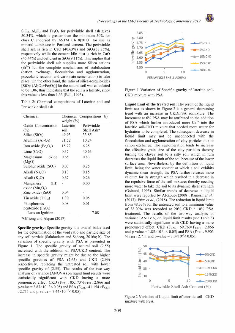
Proceedings of the OAU Faculty of Technology Conference 2019
209
SiO2, Al2O3 and Fe2O3 for periwinkle shell ash gives 50.34%, which is greater than the minimum 50% for class C endorsed by ASTM C618(2013) for use as mineral admixture in Portland cement. The periwinkle shell ash is rich in CaO (40.63%) and SiO2(33.85%), respectively while the cement kiln dust is rich in CaO (45.44%) and deficient in SiO2(9.11%). This implies that the periwinkle shell ash supplies more Silica cations (Si2+) for the complete mechanisms of stabilization (cation exchange, flocculation and agglomeration, pozzolanic reaction and carbonate cementation) to take place. On the other hand, the ratio of silica-sesquioxides [SiO2/ (Al2O3+Fe2O3)] for the natural soil was calculated to be 1.06, thus indicating that the soil is a laterite, since this value is less than 1.33 (Bell, 1993).
Table 2: Chemical compositions of Lateritic soil and Periwinkle shell ash
Chemical Chemical Compositions by weight (%)
Oxide Concentration (%)
Lateritic soil
Periwinkle Shell Ash*
Silica (SiO2) 49.93 33.85 Alumina (Al2O3) 31.52 10.24 Iron oxide (Fe2O3) 15.72 6.25 Lime (CaO) 0.37 40.63 Magnesium oxide (MgO)
0.65 0.83
Sulphur oxide (SO3) 0.03 0.25 Alkali (Na2O) 0.13 0.15 Alkali (K2O) 0.67 0.26 Manganese (III) oxide (Mn2O3)
- 0.00
Zinc oxide (ZnO) 0.04 - Tin oxide (TiO2) 1.30 0.05 Phosphorous pentoxide (P2O5)
0.08 0.01
Loss on Ignition - 7.08 *Offiong and Akpan (2017)
Specific gravity: Specific gravity is a crucial index used for the determination of the void ratio and particle size of any soil particle (Salahudeen and Sadeeq, 2016a; b). The variation of specific gravity with PSA is presented in Figure 1. The specific gravity of natural soil (2.55) increased with the addition of PSA/CKD content. The increase in specific gravity might be due to the higher specific gravities of PSA (2.65) and CKD (2.99) respectively, replacing the untreated soil with lower specific gravity of (2.55). The results of the two-way analysis of variance (ANOVA) on liquid limit results were statistically significant with CKD having a more pronounced effect. CKD (FCAL = 85.173>FCRIT = 2.866 and p-value = 2.87×10⁻¹² ˂ 0.05) and PSA (FCAL = 41.154 >FCRIT
= 2.711 and p-value = 7.44×10⁻¹⁰˂ 0.05).
Figure 1 Variation of Specific gravity of lateritic soil-CKD mixture with PSA
Liquid limit of the treated soil: The result of the liquid limit test as shown in Figure 2 is a general decreasing trend with an increase in CKD/PSA admixture. The increment at 6% PSA may be attributed to the addition of PSA which further introduced more Ca2+ into the lateritic soil-CKD mixture that needed more water for hydration to be completed. The subsequent decrease in liquid limit may not be unconnected with the flocculation and agglomeration of clay particles due to cation exchange. The agglomeration tends to increase the effective grain size of the clay particles thereby turning the clayey soil to a silty soil which in turn decreases the liquid limit of the soil because of the lower surface area. Nevertheless, by the definition of liquid limit, being the water content at which a soil exhibits dynamic shear strength, the PSA further releases more calcium for its strength which resulted in a decrease in the repulsive force of the soil mixture; thereby needing more water to take the soil to its dynamic shear strength (Osinubi, 1995). Similar trends of decrease in liquid limit were reported by Al-Zoubi (2008); Ramesh et al., (2013); Etim et al., (2018). The reduction in liquid limit from 48.33% for the untreated soil to a minimum value of 38.20% was recorded at 20% CKD / 10% PSA treatment. The results of the two-way analysis of variance (ANOVA) on liquid limit results (see Table 3) were statistically significant with CKD having a more pronounced effect. CKD (FCAL = 69.760>FCRIT = 2.866 and p-value = 1.85×10⁻¹¹ ˂ 0.05) and PSA (FCAL = 9.903 >FCRIT = 2.711 and p-value = 7.0×10⁻⁵˂ 0.05).
Figure 2 Variation of Liquid limit of lateritic soil CKD
mixture with PSA.
2.50
2.55
2.60
2.65
2.70
2.75
2.80
2.85
0 5 1 0
spec
ific
gra
vity
PERIWINKLE SHELL ASH(%)
0%CKD
5%CKD
10%CKD
15%CKD
20%CKD
30
35
40
45
50
0 5 1 0
Liqu
id L
imit
(%)
Periwinkle Shell Ash Content (%)
0%CKD
5%CKD
10%CKD
15%CKD
20%CKD
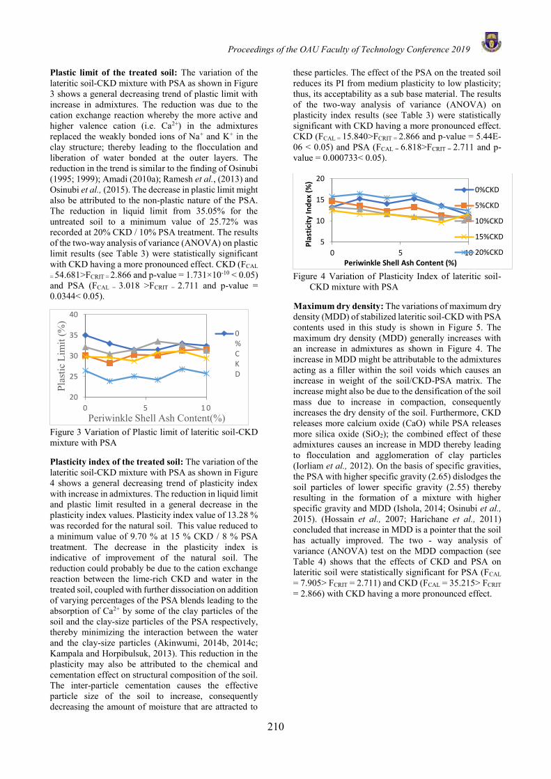
Proceedings of the OAU Faculty of Technology Conference 2019
210
Plastic limit of the treated soil: The variation of the lateritic soil-CKD mixture with PSA as shown in Figure 3 shows a general decreasing trend of plastic limit with increase in admixtures. The reduction was due to the cation exchange reaction whereby the more active and higher valence cation (i.e. Ca2+) in the admixtures replaced the weakly bonded ions of Na+ and K+ in the clay structure; thereby leading to the flocculation and liberation of water bonded at the outer layers. The reduction in the trend is similar to the finding of Osinubi (1995; 1999); Amadi (2010a); Ramesh et al., (2013) and Osinubi et al., (2015). The decrease in plastic limit might also be attributed to the non-plastic nature of the PSA. The reduction in liquid limit from 35.05% for the untreated soil to a minimum value of 25.72% was recorded at 20% CKD / 10% PSA treatment. The results of the two-way analysis of variance (ANOVA) on plastic limit results (see Table 3) were statistically significant with CKD having a more pronounced effect. CKD (FCAL
= 54.681>FCRIT = 2.866 and p-value = 1.731×10⁻¹⁰ ˂ 0.05) and PSA (FCAL = 3.018 >FCRIT = 2.711 and p-value = 0.0344˂ 0.05).
Figure 3 Variation of Plastic limit of lateritic soil-CKD mixture with PSA Plasticity index of the treated soil: The variation of the lateritic soil-CKD mixture with PSA as shown in Figure 4 shows a general decreasing trend of plasticity index with increase in admixtures. The reduction in liquid limit and plastic limit resulted in a general decrease in the plasticity index values. Plasticity index value of 13.28 % was recorded for the natural soil. This value reduced to a minimum value of 9.70 % at 15 % CKD / 8 % PSA treatment. The decrease in the plasticity index is indicative of improvement of the natural soil. The reduction could probably be due to the cation exchange reaction between the lime-rich CKD and water in the treated soil, coupled with further dissociation on addition of varying percentages of the PSA blends leading to the absorption of Ca2+ by some of the clay particles of the soil and the clay-size particles of the PSA respectively, thereby minimizing the interaction between the water and the clay-size particles (Akinwumi, 2014b, 2014c; Kampala and Horpibulsuk, 2013). This reduction in the plasticity may also be attributed to the chemical and cementation effect on structural composition of the soil. The inter-particle cementation causes the effective particle size of the soil to increase, consequently decreasing the amount of moisture that are attracted to
these particles. The effect of the PSA on the treated soil reduces its PI from medium plasticity to low plasticity; thus, its acceptability as a sub base material. The results of the two-way analysis of variance (ANOVA) on plasticity index results (see Table 3) were statistically significant with CKD having a more pronounced effect. CKD (FCAL = 15.840>FCRIT = 2.866 and p-value = 5.44E-06 ˂ 0.05) and PSA (FCAL = 6.818>FCRIT = 2.711 and p-value = 0.000733˂ 0.05).
Figure 4 Variation of Plasticity Index of lateritic soil-
CKD mixture with PSA
Maximum dry density: The variations of maximum dry density (MDD) of stabilized lateritic soil-CKD with PSA contents used in this study is shown in Figure 5. The maximum dry density (MDD) generally increases with an increase in admixtures as shown in Figure 4. The increase in MDD might be attributable to the admixtures acting as a filler within the soil voids which causes an increase in weight of the soil/CKD-PSA matrix. The increase might also be due to the densification of the soil mass due to increase in compaction, consequently increases the dry density of the soil. Furthermore, CKD releases more calcium oxide (CaO) while PSA releases more silica oxide (SiO2); the combined effect of these admixtures causes an increase in MDD thereby leading to flocculation and agglomeration of clay particles (Iorliam et al., 2012). On the basis of specific gravities, the PSA with higher specific gravity (2.65) dislodges the soil particles of lower specific gravity (2.55) thereby resulting in the formation of a mixture with higher specific gravity and MDD (Ishola, 2014; Osinubi et al., 2015). (Hossain et al., 2007; Harichane et al., 2011) concluded that increase in MDD is a pointer that the soil has actually improved. The two - way analysis of variance (ANOVA) test on the MDD compaction (see Table 4) shows that the effects of CKD and PSA on lateritic soil were statistically significant for PSA (FCAL = 7.905> FCRIT = 2.711) and CKD (FCAL = 35.215> FCRIT = 2.866) with CKD having a more pronounced effect.
20
25
30
35
40
0 5 1 0
Plas
tic L
imit
(%)
Periwinkle Shell Ash Content(%)
0%CKD
5
10
15
20
0 5 10
Pla
stic
ity
Ind
ex
(%)
Periwinkle Shell Ash Content (%)
0%CKD
5%CKD
10%CKD
15%CKD
20%CKD
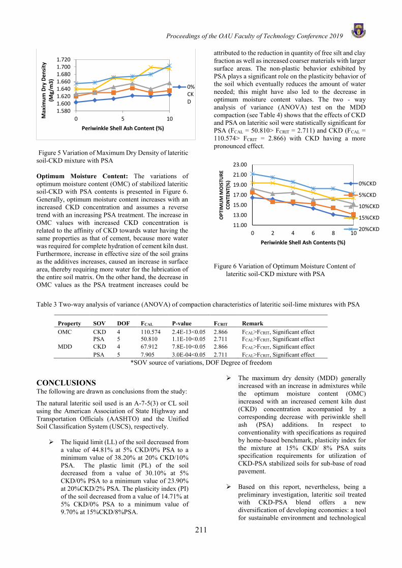
Proceedings of the OAU Faculty of Technology Conference 2019
211
Figure 5 Variation of Maximum Dry Density of lateritic soil-CKD mixture with PSA Optimum Moisture Content: The variations of optimum moisture content (OMC) of stabilized lateritic soil-CKD with PSA contents is presented in Figure 6. Generally, optimum moisture content increases with an increased CKD concentration and assumes a reverse trend with an increasing PSA treatment. The increase in OMC values with increased CKD concentration is related to the affinity of CKD towards water having the same properties as that of cement, because more water was required for complete hydration of cement kiln dust. Furthermore, increase in effective size of the soil grains as the additives increases, caused an increase in surface area, thereby requiring more water for the lubrication of the entire soil matrix. On the other hand, the decrease in OMC values as the PSA treatment increases could be
attributed to the reduction in quantity of free silt and clay fraction as well as increased coarser materials with larger surface areas. The non-plastic behavior exhibited by PSA plays a significant role on the plasticity behavior of the soil which eventually reduces the amount of water needed; this might have also led to the decrease in optimum moisture content values. The two - way analysis of variance (ANOVA) test on the MDD compaction (see Table 4) shows that the effects of CKD and PSA on lateritic soil were statistically significant for PSA (FCAL = 50.810> FCRIT = 2.711) and CKD (FCAL = 110.574> FCRIT = 2.866) with CKD having a more pronounced effect.
Figure 6 Variation of Optimum Moisture Content of lateritic soil-CKD mixture with PSA
Table 3 Two-way analysis of variance (ANOVA) of compaction characteristics of lateritic soil-lime mixtures with PSA
Property SOV DOF FCAL P-value FCRIT Remark OMC CKD 4 110.574 2.4E-13<0.05 2.866 FCAL>FCRIT, Significant effect PSA 5 50.810 1.1E-10<0.05 2.711 FCAL>FCRIT, Significant effect MDD CKD 4 67.912 7.8E-10<0.05 2.866 FCAL>FCRIT, Significant effect PSA 5 7.905 3.0E-04<0.05 2.711 FCAL>FCRIT, Significant effect
*SOV source of variations, DOF Degree of freedom
CONCLUSIONS The following are drawn as conclusions from the study:
The natural lateritic soil used is an A-7-5(3) or CL soil using the American Association of State Highway and Transportation Officials (AASHTO) and the Unified Soil Classification System (USCS), respectively.
The liquid limit (LL) of the soil decreased from a value of 44.81% at 5% CKD/0% PSA to a minimum value of 38.20% at 20% CKD/10% PSA. The plastic limit (PL) of the soil decreased from a value of 30.10% at 5% CKD/0% PSA to a minimum value of 23.90% at 20%CKD/2% PSA. The plasticity index (PI) of the soil decreased from a value of 14.71% at 5% CKD/0% PSA to a minimum value of 9.70% at 15%CKD/8%PSA.
The maximum dry density (MDD) generally increased with an increase in admixtures while the optimum moisture content (OMC) increased with an increased cement kiln dust (CKD) concentration accompanied by a corresponding decrease with periwinkle shell ash (PSA) additions. In respect to conventionality with specifications as required by home-based benchmark, plasticity index for the mixture at 15% CKD/ 8% PSA suits specification requirements for utilization of CKD-PSA stabilized soils for sub-base of road pavement.
Based on this report, nevertheless, being a
preliminary investigation, lateritic soil treated with CKD-PSA blend offers a new diversification of developing economies: a tool for sustainable environment and technological
1.5801.6001.6201.6401.6601.6801.7001.720
0 5 10Max
imu
m D
ry D
en
sity
(M
g/m
3)
Periwinkle Shell Ash Content (%)
0%CKD
11.00
13.00
15.00
17.00
19.00
21.00
23.00
0 2 4 6 8 10
OP
TIM
UM
MO
ISTU
RE
CO
NTE
NT(
%)
Periwinkle Shell Ash Contents (%)
0%CKD
5%CKD
10%CKD
15%CKD
20%CKD
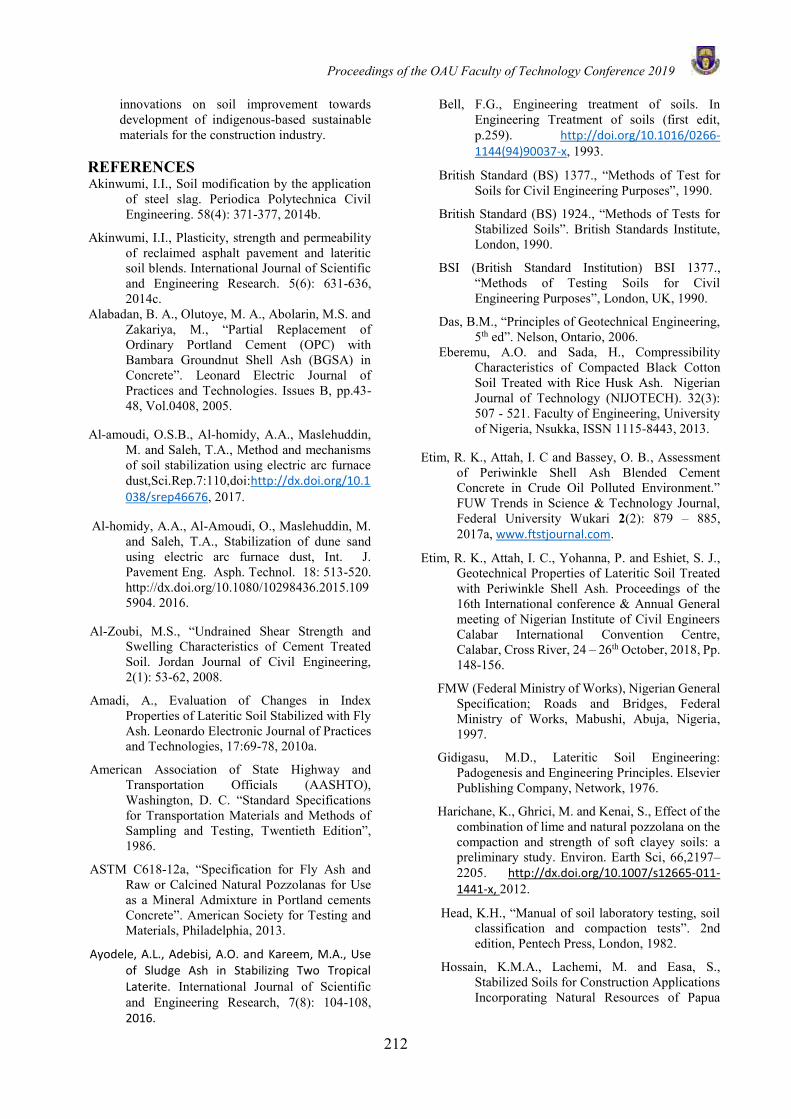
Proceedings of the OAU Faculty of Technology Conference 2019
212
innovations on soil improvement towards development of indigenous-based sustainable materials for the construction industry.
REFERENCES Akinwumi, I.I., Soil modification by the application
of steel slag. Periodica Polytechnica Civil Engineering. 58(4): 371-377, 2014b.
Akinwumi, I.I., Plasticity, strength and permeability of reclaimed asphalt pavement and lateritic soil blends. International Journal of Scientific and Engineering Research. 5(6): 631-636, 2014c.
Alabadan, B. A., Olutoye, M. A., Abolarin, M.S. and Zakariya, M., “Partial Replacement of Ordinary Portland Cement (OPC) with Bambara Groundnut Shell Ash (BGSA) in Concrete”. Leonard Electric Journal of Practices and Technologies. Issues B, pp.43-48, Vol.0408, 2005.
Al-amoudi, O.S.B., Al-homidy, A.A., Maslehuddin, M. and Saleh, T.A., Method and mechanisms of soil stabilization using electric arc furnace dust,Sci.Rep.7:110,doi:http://dx.doi.org/10.1038/srep46676, 2017.
Al-homidy, A.A., Al-Amoudi, O., Maslehuddin, M. and Saleh, T.A., Stabilization of dune sand using electric arc furnace dust, Int. J. Pavement Eng. Asph. Technol. 18: 513-520. http://dx.doi.org/10.1080/10298436.2015.1095904. 2016.
Al-Zoubi, M.S., “Undrained Shear Strength and Swelling Characteristics of Cement Treated Soil. Jordan Journal of Civil Engineering, 2(1): 53-62, 2008.
Amadi, A., Evaluation of Changes in Index Properties of Lateritic Soil Stabilized with Fly Ash. Leonardo Electronic Journal of Practices and Technologies, 17:69-78, 2010a.
American Association of State Highway and Transportation Officials (AASHTO), Washington, D. C. “Standard Specifications for Transportation Materials and Methods of Sampling and Testing, Twentieth Edition”, 1986.
ASTM C618-12a, “Specification for Fly Ash and Raw or Calcined Natural Pozzolanas for Use as a Mineral Admixture in Portland cements Concrete”. American Society for Testing and Materials, Philadelphia, 2013.
Ayodele, A.L., Adebisi, A.O. and Kareem, M.A., Use of Sludge Ash in Stabilizing Two Tropical Laterite. International Journal of Scientific and Engineering Research, 7(8): 104-108, 2016.
Bell, F.G., Engineering treatment of soils. In Engineering Treatment of soils (first edit, p.259). http://doi.org/10.1016/0266-1144(94)90037-x, 1993.
British Standard (BS) 1377., “Methods of Test for Soils for Civil Engineering Purposes”, 1990.
British Standard (BS) 1924., “Methods of Tests for Stabilized Soils”. British Standards Institute, London, 1990.
BSI (British Standard Institution) BSI 1377., “Methods of Testing Soils for Civil Engineering Purposes”, London, UK, 1990.
Das, B.M., “Principles of Geotechnical Engineering, 5th ed”. Nelson, Ontario, 2006.
Eberemu, A.O. and Sada, H., Compressibility Characteristics of Compacted Black Cotton Soil Treated with Rice Husk Ash. Nigerian Journal of Technology (NIJOTECH). 32(3): 507 - 521. Faculty of Engineering, University of Nigeria, Nsukka, ISSN 1115-8443, 2013.
Etim, R. K., Attah, I. C and Bassey, O. B., Assessment of Periwinkle Shell Ash Blended Cement Concrete in Crude Oil Polluted Environment.” FUW Trends in Science & Technology Journal, Federal University Wukari 2(2): 879 – 885, 2017a, www.ftstjournal.com.
Etim, R. K., Attah, I. C., Yohanna, P. and Eshiet, S. J., Geotechnical Properties of Lateritic Soil Treated with Periwinkle Shell Ash. Proceedings of the 16th International conference & Annual General meeting of Nigerian Institute of Civil Engineers Calabar International Convention Centre, Calabar, Cross River, 24 – 26th October, 2018, Pp. 148-156.
FMW (Federal Ministry of Works), Nigerian General Specification; Roads and Bridges, Federal Ministry of Works, Mabushi, Abuja, Nigeria, 1997.
Gidigasu, M.D., Lateritic Soil Engineering: Padogenesis and Engineering Principles. Elsevier Publishing Company, Network, 1976.
Harichane, K., Ghrici, M. and Kenai, S., Effect of the combination of lime and natural pozzolana on the compaction and strength of soft clayey soils: a preliminary study. Environ. Earth Sci, 66,2197–2205. http://dx.doi.org/10.1007/s12665-011-1441-x, 2012.
Head, K.H., “Manual of soil laboratory testing, soil classification and compaction tests”. 2nd edition, Pentech Press, London, 1982.
Hossain, K.M.A., Lachemi, M. and Easa, S., Stabilized Soils for Construction Applications Incorporating Natural Resources of Papua
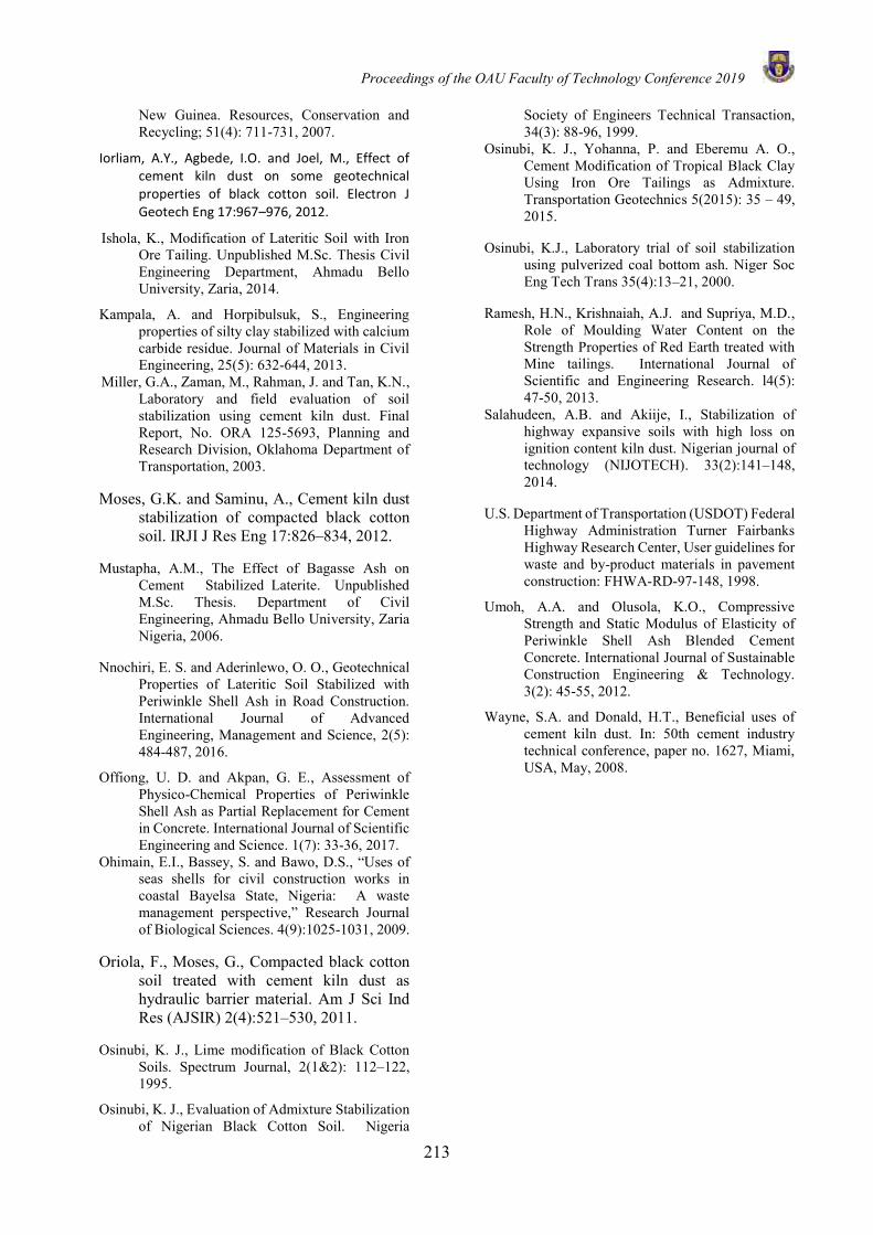
Proceedings of the OAU Faculty of Technology Conference 2019
213
New Guinea. Resources, Conservation and Recycling; 51(4): 711-731, 2007.
Iorliam, A.Y., Agbede, I.O. and Joel, M., Effect of cement kiln dust on some geotechnical properties of black cotton soil. Electron J Geotech Eng 17:967–976, 2012.
Ishola, K., Modification of Lateritic Soil with Iron Ore Tailing. Unpublished M.Sc. Thesis Civil Engineering Department, Ahmadu Bello University, Zaria, 2014.
Kampala, A. and Horpibulsuk, S., Engineering properties of silty clay stabilized with calcium carbide residue. Journal of Materials in Civil Engineering, 25(5): 632-644, 2013.
Miller, G.A., Zaman, M., Rahman, J. and Tan, K.N., Laboratory and field evaluation of soil stabilization using cement kiln dust. Final Report, No. ORA 125-5693, Planning and Research Division, Oklahoma Department of Transportation, 2003.
Moses, G.K. and Saminu, A., Cement kiln dust stabilization of compacted black cotton soil. IRJI J Res Eng 17:826–834, 2012.
Mustapha, A.M., The Effect of Bagasse Ash on Cement Stabilized Laterite. Unpublished M.Sc. Thesis. Department of Civil Engineering, Ahmadu Bello University, Zaria Nigeria, 2006.
Nnochiri, E. S. and Aderinlewo, O. O., Geotechnical Properties of Lateritic Soil Stabilized with Periwinkle Shell Ash in Road Construction. International Journal of Advanced Engineering, Management and Science, 2(5): 484-487, 2016.
Offiong, U. D. and Akpan, G. E., Assessment of Physico-Chemical Properties of Periwinkle Shell Ash as Partial Replacement for Cement in Concrete. International Journal of Scientific Engineering and Science. 1(7): 33-36, 2017.
Ohimain, E.I., Bassey, S. and Bawo, D.S., “Uses of seas shells for civil construction works in coastal Bayelsa State, Nigeria: A waste management perspective,” Research Journal of Biological Sciences. 4(9):1025-1031, 2009.
Oriola, F., Moses, G., Compacted black cotton soil treated with cement kiln dust as hydraulic barrier material. Am J Sci Ind Res (AJSIR) 2(4):521–530, 2011.
Osinubi, K. J., Lime modification of Black Cotton Soils. Spectrum Journal, 2(1&2): 112–122, 1995.
Osinubi, K. J., Evaluation of Admixture Stabilization of Nigerian Black Cotton Soil. Nigeria
Society of Engineers Technical Transaction, 34(3): 88-96, 1999.
Osinubi, K. J., Yohanna, P. and Eberemu A. O., Cement Modification of Tropical Black Clay Using Iron Ore Tailings as Admixture. Transportation Geotechnics 5(2015): 35 – 49, 2015.
Osinubi, K.J., Laboratory trial of soil stabilization using pulverized coal bottom ash. Niger Soc Eng Tech Trans 35(4):13–21, 2000.
Ramesh, H.N., Krishnaiah, A.J. and Supriya, M.D., Role of Moulding Water Content on the Strength Properties of Red Earth treated with Mine tailings. International Journal of Scientific and Engineering Research. l4(5): 47-50, 2013.
Salahudeen, A.B. and Akiije, I., Stabilization of highway expansive soils with high loss on ignition content kiln dust. Nigerian journal of technology (NIJOTECH). 33(2):141–148, 2014.
U.S. Department of Transportation (USDOT) Federal Highway Administration Turner Fairbanks Highway Research Center, User guidelines for waste and by-product materials in pavement construction: FHWA‐RD‐97‐148, 1998.
Umoh, A.A. and Olusola, K.O., Compressive Strength and Static Modulus of Elasticity of Periwinkle Shell Ash Blended Cement Concrete. International Journal of Sustainable Construction Engineering & Technology. 3(2): 45-55, 2012.
Wayne, S.A. and Donald, H.T., Beneficial uses of cement kiln dust. In: 50th cement industry technical conference, paper no. 1627, Miami, USA, May, 2008.
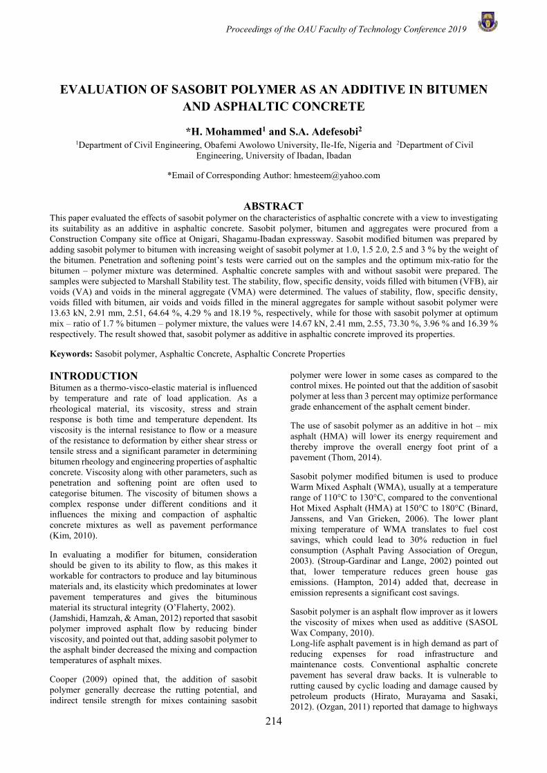
Proceedings of the OAU Faculty of Technology Conference 2019
214
EVALUATION OF SASOBIT POLYMER AS AN ADDITIVE IN BITUMEN AND ASPHALTIC CONCRETE
*H. Mohammed1 and S.A. Adefesobi2 1Department of Civil Engineering, Obafemi Awolowo University, Ile-Ife, Nigeria and 2Department of Civil
Engineering, University of Ibadan, Ibadan
*Email of Corresponding Author: [email protected]
ABSTRACT This paper evaluated the effects of sasobit polymer on the characteristics of asphaltic concrete with a view to investigating its suitability as an additive in asphaltic concrete. Sasobit polymer, bitumen and aggregates were procured from a Construction Company site office at Onigari, Shagamu-Ibadan expressway. Sasobit modified bitumen was prepared by adding sasobit polymer to bitumen with increasing weight of sasobit polymer at 1.0, 1.5 2.0, 2.5 and 3 % by the weight of the bitumen. Penetration and softening point’s tests were carried out on the samples and the optimum mix-ratio for the bitumen – polymer mixture was determined. Asphaltic concrete samples with and without sasobit were prepared. The samples were subjected to Marshall Stability test. The stability, flow, specific density, voids filled with bitumen (VFB), air voids (VA) and voids in the mineral aggregate (VMA) were determined. The values of stability, flow, specific density, voids filled with bitumen, air voids and voids filled in the mineral aggregates for sample without sasobit polymer were 13.63 kN, 2.91 mm, 2.51, 64.64 %, 4.29 % and 18.19 %, respectively, while for those with sasobit polymer at optimum mix – ratio of 1.7 % bitumen – polymer mixture, the values were 14.67 kN, 2.41 mm, 2.55, 73.30 %, 3.96 % and 16.39 % respectively. The result showed that, sasobit polymer as additive in asphaltic concrete improved its properties.
Keywords: Sasobit polymer, Asphaltic Concrete, Asphaltic Concrete Properties INTRODUCTION Bitumen as a thermo-visco-elastic material is influenced by temperature and rate of load application. As a rheological material, its viscosity, stress and strain response is both time and temperature dependent. Its viscosity is the internal resistance to flow or a measure of the resistance to deformation by either shear stress or tensile stress and a significant parameter in determining bitumen rheology and engineering properties of asphaltic concrete. Viscosity along with other parameters, such as penetration and softening point are often used to categorise bitumen. The viscosity of bitumen shows a complex response under different conditions and it influences the mixing and compaction of asphaltic concrete mixtures as well as pavement performance (Kim, 2010). In evaluating a modifier for bitumen, consideration should be given to its ability to flow, as this makes it workable for contractors to produce and lay bituminous materials and, its elasticity which predominates at lower pavement temperatures and gives the bituminous material its structural integrity (O’Flaherty, 2002). (Jamshidi, Hamzah, & Aman, 2012) reported that sasobit polymer improved asphalt flow by reducing binder viscosity, and pointed out that, adding sasobit polymer to the asphalt binder decreased the mixing and compaction temperatures of asphalt mixes. Cooper (2009) opined that, the addition of sasobit polymer generally decrease the rutting potential, and indirect tensile strength for mixes containing sasobit
polymer were lower in some cases as compared to the control mixes. He pointed out that the addition of sasobit polymer at less than 3 percent may optimize performance grade enhancement of the asphalt cement binder. The use of sasobit polymer as an additive in hot – mix asphalt (HMA) will lower its energy requirement and thereby improve the overall energy foot print of a pavement (Thom, 2014). Sasobit polymer modified bitumen is used to produce Warm Mixed Asphalt (WMA), usually at a temperature range of 110°C to 130°C, compared to the conventional Hot Mixed Asphalt (HMA) at 150°C to 180°C (Binard, Janssens, and Van Grieken, 2006). The lower plant mixing temperature of WMA translates to fuel cost savings, which could lead to 30% reduction in fuel consumption (Asphalt Paving Association of Oregun, 2003). (Stroup-Gardinar and Lange, 2002) pointed out that, lower temperature reduces green house gas emissions. (Hampton, 2014) added that, decrease in emission represents a significant cost savings. Sasobit polymer is an asphalt flow improver as it lowers the viscosity of mixes when used as additive (SASOL Wax Company, 2010). Long-life asphalt pavement is in high demand as part of reducing expenses for road infrastructure and maintenance costs. Conventional asphaltic concrete pavement has several draw backs. It is vulnerable to rutting caused by cyclic loading and damage caused by petroleum products (Hirato, Murayama and Sasaki, 2012). (Ozgan, 2011) reported that damage to highways
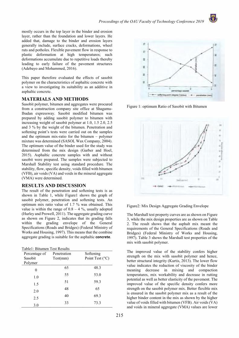
Proceedings of the OAU Faculty of Technology Conference 2019
215
mostly occurs in the top layer in the binder and erosion layer, rather than the foundation and lower layers. He added that, damage to the binder and erosion layers generally include, surface cracks, deformations, wheel ruts and potholes. Flexible pavement flow in response to plastic deformation at high temperatures; such deformations accumulate due to repetitive loads thereby leading to early failure of the pavement structures (Adebayo and Mohammed, 2016). This paper therefore evaluated the effects of sasobit polymer on the characteristics of asphaltic concrete with a view to investigating its suitability as an additive in asphaltic concrete.
MATERIALS AND METHODS Sasobit polymer, bitumen and aggregates were procured from a construction company site office at Shagamu-Ibadan expressway. Sasobit modified bitumen was prepared by adding sasobit polymer to bitumen with increasing weight of sasobit polymer at 1.0, 1.5 2.0, 2.5 and 3 % by the weight of the bitumen. Penetration and softening point’s tests were carried out on the samples and the optimum mix-ratio for the bitumen – polymer mixture was determined (SASOL Wax Company, 2004). The optimum value of the binder used for the study was determined from the mix design (Garber and Hoel, 2015). Asphaltic concrete samples with and without sasobit were prepared. The samples were subjected to Marshall Stability test using standard procedure. The stability, flow, specific density, voids filled with bitumen (VFB), air voids (VA) and voids in the mineral aggregate (VMA) were determined.
RESULTS AND DISCUSSION The result of the penetration and softening tests is as shown in Table 1, while Figure1 shows the graph of sasobit polymer, penetration and softening tests. An optimum mix ratio value of 1.7 % was obtained. This value is within the range of 0.8 – 4 %, usually adopted (Hurley and Prowell, 2011). The aggregate grading curve as shown on Figure 2, indicates that its grading falls within the grading envelope of the General Specifications (Roads and Bridges) (Federal Ministry of Works and Housing, 1997). This means that the combine aggregate grading is suitable for the asphaltic concrete.
Table1: Bitumen Test Results
Percentage of Sasobit Polymer
Penetration Test(mm)
Softening Point Test (°C)
0 65 48.3
1.0 55 53.0
1.5 51 59.3
2.0 48 65
2.5 40 69.3
3.0 33 73.3
Figure 1: optimum Ratio of Sasobit with Bitumen
Figure2: Mix Design Aggregate Grading Envelope
The Marshall test property curves are as shown on Figure 3, while the mix design properties are as shown on Table 2. The result shows that the asphalt mix meant the requirements of the General Specifications (Roads and Bridges) (Federal Ministry of Works and Housing, 1997). Table 3 shows the Marshall test properties of the mix with sasobit polymer. The improved value of the stability confers higher strength on the mix with sasobit polymer and hence, better structural integrity (Kurtis, 2013). The lower flow value indicates the reduction of viscosity of the binder meaning decrease in mixing and compaction temperatures, mix workability and decrease in rutting potential as well as better elasticity of the pavement. The improved value of the specific density confers more strength on the sasobit polymer mix. Better flexible mix is ensured in the sasobit polymer mix as a result of the higher binder content in the mix as shown by the higher value of voids filled with bitumen (VFB). Air voids (VA) and voids in mineral aggregate (VMA) values are lower
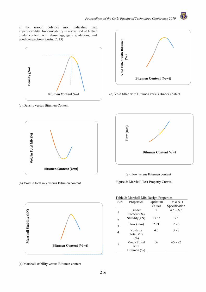
Proceedings of the OAU Faculty of Technology Conference 2019
216
in the sasobit polymer mix; indicating mix impermeability. Impermeability is maximised at higher binder content, with dense aggregate gradations, and good compaction (Kurtis, 2013)
(a) Density versus Bitumen Content
(b) Void in total mix versus Bitumen content
(c) Marshall stability versus Bitumen content
(d) Void filled with Bitumen versus Binder content
(e) Flow versus Bitumen content
Figure 3: Marshall Test Property Curves Table 2: Marshall Mix Design Properties
S/N Properties Optimum Values
FMW&H Specification
1 Binder Content (%)
5 4.5 – 6.5
2 Stability(kN) 13.63 3.5
3 Flow (mm) 2.91 2 - 6
4 Voids in Total Mix
(%)
4.5 3 - 8
5 Voids Filled with
Bitumen (%)
66 65 - 72
De
nsi
ty g
/mL
Bitumen Content %wt
Vo
id in
To
tal M
ix (
%)
Bitumen Content (%wt)
Mar
shal
l Sta
bilit
y (k
N)
Bitumen Content (%wt)
Voi
d Fi
lled
with
Bitu
men
(%
)
Bitumen Content (%wt)
Flow
(mm
)
Bitumen Content %wt
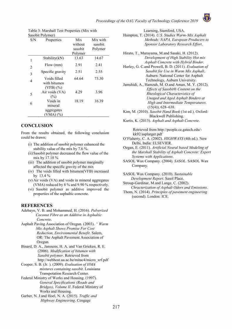
Proceedings of the OAU Faculty of Technology Conference 2019
217
Table 3: Marshall Test Properties (Mix with Sasobit Polymer)
S/N Properties Mix without sasobit
Polymer
Mix with sasobit
Polymer
1 Stability(kN) 13.63 14.67
2 Flow (mm) 2.91 2.41
3 Specific gravity 2.51 2.55
4 Voids filled with bitumen (VFB) (%)
64.64 73.30
5 Air voids (VA) (%)
4.29 3.96
6 Voids in mineral
aggregates (VMA) (%)
18.19 16.39
CONCLUSION From the results obtained, the following conclusion could be drawn;
(i) The addition of sasobit polymer enhanced the stability value of the mix by 7.6 %.
(ii) Sasobit polymer decreased the flow value of the mix by 17.18 %
(iii) The addition of sasobit polymer marginally affected the specific gravity of the mix
(iv) The voids filled with bitumen(VFB) increased by 13.4 %
(v) Air voids (VA) and voids in mineral aggregates (VMA) reduced by 8 % and 9.90 % respectively.
(vi) Sasobit polymer as additive improved the properties of the asphaltic concrete.
REFERENCES Adebayo, V. B. and Mohammed, H. (2016). Pulverized Coconut Fibre as an Additive in Asphaltic Concrete. Asphalt Paving Association of Oregun. (2003). “ Warm Mix Asphalt Shows Promise For Cost Reduction, Environmental Benefit. Salem, OR: The Asphalt Pavement Association of Oregun. Binard, D. A., Janssens, H. A. and Van Grieken, R. E. (2006). Modification of bitumen with Sasobit polymer. Retrieved from http://webhost.ua.ac.be/mitac4/micro_xrf.pdf Cooper, S. B. (Jr. ). (2009). Evaluation of HMA mixtures containing sasobit. Louisiana Transpotation Research Center. Federal Ministry of Works and Housing. (1997). General Specifications (Roads and Bridges), Volume II. Federal Ministry of Works and Housing. Garber, N. J.and Hoel, N. A. (2015). Traffic and Highway Engineering. Cengage
Learning, Stamford, USA. Hampton, T. (2014). U.S. Studies Warm-Mix Asphalt Methods: NAPA, European Producers to Sponsor Laboratory Research Effort. Hirato, T., Murayama, M.and Sasaki, H. (2012). Development of High Stability Hot mix Asphalt Concrete with Hybrid Binder. Hurley, G. C.and Prowell, B. D. (2011). Evaluation of Sasobit for Use in Warm Mix Asphalt. Auburn: National Center for Asphalt Technology, Auburn University. Jamshidi, A., Hamzah, M. O.and Aman, M. Y. (2012). Effects of Sasobit® Content on the Rheological Characteristics of Unaged and Aged Asphalt Binders at High and Intermediate Temperatures. (15(4)), 628–638. Kim, M. (2010). Sasobit Hand Book (1st ed.). Oxford: Blackwell Publishing. Kurtis, K. (2013). Asphalt and Asphalt Concrete. Retrieved from http://people.ce.gatech.edu/- kk92/asplarger.pdf O’Flaherty, C. A. (2002). HIGHWAYS (4th ed.). New Delhi, India: ELSEVIER. Ozgan, E. (2011). Artificial Neural based Modeling of the Marshall Stability of Asphalt Concrete: Expert Systems with Applications. SASOL Wax Company. (2004). SASOL. SASOL Wax Company.
SASOL Wax Company. (2010). Sustainable Development Report. Sasol Place. Stroup-Gardinar, M.and Lange, C. (2002). Chracterization of Asphalt Odors and Emissions. Thom, N. (2014). Principles of pavement engineering (second). London: ICE.
Proceedings of the OAU Faculty of Technology Conference 2019
218
FULFILLING BIOMASS DRYING REQUIREMENT FOR SUSTAINABLE DEVELOPMENT OF BIOENERGY: A COMPARATIVE STUDY OF OPEN
SUN, SOLAR AND HOT AIR DRYING OF ORANGE WASTE
O. O. Agbede*1, A. O. Adebiyi1, E.O. Oke2, K. A. Babatunde1, F.N. Osuolale1, O.O. Ogunleye1, S. E. Agarry1 and A.O. Arinkoola1
1 Department of Chemical Engineering, Ladoke Akintola University of Technology, P.M.B. 4000, Ogbomoso, Nigeria. 2 Department of Chemical Engineering, Michael Okpara University of Agriculture, Umudike, Nigeria
*Email of Corresponding Author: [email protected]
ABSTRACT The thermochemical conversion of biomass to bioenergy through pyrolysis, gasification and combustion may require the removal of moisture from the biomass by drying before the conversion process. This drying step, an energy intensive operation, is essential to the overall efficiency, economic viability and sustainability of biomass conversion to bioenergy. Hence, this study investigated the drying characteristics of biomass (orange waste) by open sun, solar and hot air drying methods. Orange waste (skin) were crushed and then dried in a hot air oven dryer (at 80, 120 and 140 oC), open sun and solar dryer; the mass of the material was measured at interval until constant mass was achieved. Hot air oven drying of orange skin took place in the falling rate period and the drying rate increased with increasing drying temperature. The effective moisture diffusivity increased with drying temperature and varied from 7.0 x 10⁻⁹ to 1.8 x 10⁻⁸ m2 s-1. The temperature dependence of the effective moisture diffusivity was suitably described by an Arrhenius-type equation and an activation energy of 16.1 kJ mol-1 was required for drying the orange skin. The specific energy required for hot air drying was 846 – 1475 kJ/g. The effective moisture diffusivities for the drying of orange skin in open sun and solar dryer were 2.0 x 10⁻⁹ and 2.16 x 10⁻⁹ m2 s-1, respectively. Orange skin dried fastest in hot air dryer compared to open sun and solar dryer, however orange skin drying energy requirement can be cheaply provided by the sun. Keywords: Biomass, bioenergy, orange waste, drying, effective moisture diffusivity
INTRODUCTION Energy is indispensable to sustainable development. However, global energy requirement is still largely provided by non-renewable fossil fuels which are fast depleting and highly polluting (Panwar et al., 2011; Demirbas et al., 2017). Sustainable supply of energy resources coupled with effective and efficient utilization of energy resources are required for sustainable development (Dincer, 2000). Thus the quest for bioenergy is currently on the increase as a solution to the adverse effects of utilization of fossil fuel and a means of achieving sustainable development (Dincer, 2000; Ho et al., 2014). Bioenergy is renewable energy derived from biological sources or biomass. Biomass are materials derived from microorganisms, animals and plants; they include algae, energy crops, animal wastes, food wastes, wood and wood wastes, agricultural residues, municipal solid wastes and industrial residues (Demirbas et al., 2017). They are produced by the process of photosynthesis which combines solar energy and carbon dioxide into chemical energy in the form of carbohydrates, so their utilisation as a fuel is a carbon neutral process since the carbon dioxide captured during photosynthesis is released during its combustion (Kumar et al., 2009). Sustainable supply of energy resource implies that the energy resource is readily and sustainably available at
reasonable cost in the long term and can be utilized for all required tasks without causing negative societal impacts (Dincer, 2000). Biomass are renewable, readily available and their conversion to bioenergy are environmentally benign, they can also stabilize atmospheric concentrations of greenhouse gases below dangerous levels (Long et al., 2013). Hence bioenergy is essential to sustainable energy development. Sustainable development requires a reduction of dependency on fossil fuels and its associated emissions; the continuous increase in atmospheric greenhouse gases especially carbon dioxide which causes global warming and climate change associated with the utilization of fossil fuels is thus a major impetus for the development of bioenergy (Panwar et al., 2011; Demirbas et al., 2017). Biomass may be used directly or first converted into biofuel before it is utilised for transportation or electricity generation. (Ellabban et al., 2014). They can be converted into biofuels or bioenergy through thermochemical, biochemical and physicochemical processes. The thermochemical conversion processes are pyrolysis, gasification, hydrothermal liquefaction and direct combustion, the biochemical processes include fermentation, anaerobic digestion and biophotolysis while the physicochemical process involves oil extraction e.g. from seed biomass followed by transesterification (Kumar, 2009; Kumar 2015).
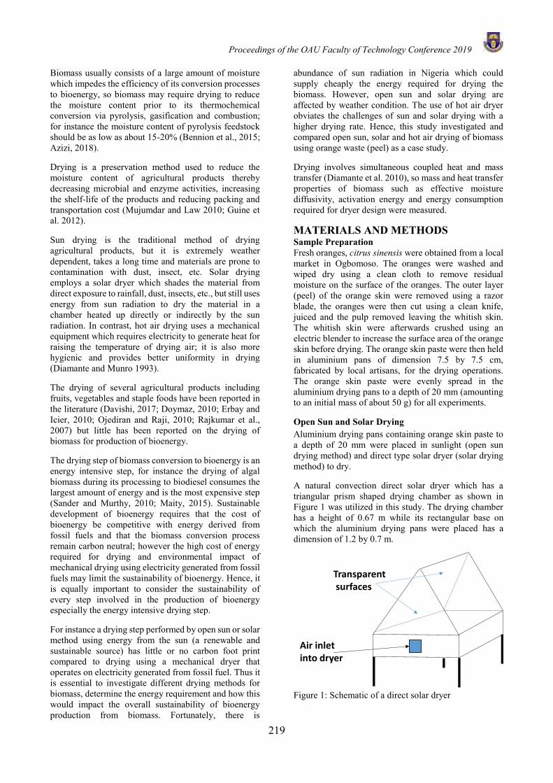
Proceedings of the OAU Faculty of Technology Conference 2019
219
Biomass usually consists of a large amount of moisture which impedes the efficiency of its conversion processes to bioenergy, so biomass may require drying to reduce the moisture content prior to its thermochemical conversion via pyrolysis, gasification and combustion; for instance the moisture content of pyrolysis feedstock should be as low as about 15-20% (Bennion et al., 2015; Azizi, 2018). Drying is a preservation method used to reduce the moisture content of agricultural products thereby decreasing microbial and enzyme activities, increasing the shelf-life of the products and reducing packing and transportation cost (Mujumdar and Law 2010; Guine et al. 2012). Sun drying is the traditional method of drying agricultural products, but it is extremely weather dependent, takes a long time and materials are prone to contamination with dust, insect, etc. Solar drying employs a solar dryer which shades the material from direct exposure to rainfall, dust, insects, etc., but still uses energy from sun radiation to dry the material in a chamber heated up directly or indirectly by the sun radiation. In contrast, hot air drying uses a mechanical equipment which requires electricity to generate heat for raising the temperature of drying air; it is also more hygienic and provides better uniformity in drying (Diamante and Munro 1993). The drying of several agricultural products including fruits, vegetables and staple foods have been reported in the literature (Davishi, 2017; Doymaz, 2010; Erbay and Icier, 2010; Ojediran and Raji, 2010; Rajkumar et al., 2007) but little has been reported on the drying of biomass for production of bioenergy. The drying step of biomass conversion to bioenergy is an energy intensive step, for instance the drying of algal biomass during its processing to biodiesel consumes the largest amount of energy and is the most expensive step (Sander and Murthy, 2010; Maity, 2015). Sustainable development of bioenergy requires that the cost of bioenergy be competitive with energy derived from fossil fuels and that the biomass conversion process remain carbon neutral; however the high cost of energy required for drying and environmental impact of mechanical drying using electricity generated from fossil fuels may limit the sustainability of bioenergy. Hence, it is equally important to consider the sustainability of every step involved in the production of bioenergy especially the energy intensive drying step. For instance a drying step performed by open sun or solar method using energy from the sun (a renewable and sustainable source) has little or no carbon foot print compared to drying using a mechanical dryer that operates on electricity generated from fossil fuel. Thus it is essential to investigate different drying methods for biomass, determine the energy requirement and how this would impact the overall sustainability of bioenergy production from biomass. Fortunately, there is
abundance of sun radiation in Nigeria which could supply cheaply the energy required for drying the biomass. However, open sun and solar drying are affected by weather condition. The use of hot air dryer obviates the challenges of sun and solar drying with a higher drying rate. Hence, this study investigated and compared open sun, solar and hot air drying of biomass using orange waste (peel) as a case study. Drying involves simultaneous coupled heat and mass transfer (Diamante et al. 2010), so mass and heat transfer properties of biomass such as effective moisture diffusivity, activation energy and energy consumption required for dryer design were measured. MATERIALS AND METHODS Sample Preparation Fresh oranges, citrus sinensis were obtained from a local market in Ogbomoso. The oranges were washed and wiped dry using a clean cloth to remove residual moisture on the surface of the oranges. The outer layer (peel) of the orange skin were removed using a razor blade, the oranges were then cut using a clean knife, juiced and the pulp removed leaving the whitish skin. The whitish skin were afterwards crushed using an electric blender to increase the surface area of the orange skin before drying. The orange skin paste were then held in aluminium pans of dimension 7.5 by 7.5 cm, fabricated by local artisans, for the drying operations. The orange skin paste were evenly spread in the aluminium drying pans to a depth of 20 mm (amounting to an initial mass of about 50 g) for all experiments. Open Sun and Solar Drying Aluminium drying pans containing orange skin paste to a depth of 20 mm were placed in sunlight (open sun drying method) and direct type solar dryer (solar drying method) to dry. A natural convection direct solar dryer which has a triangular prism shaped drying chamber as shown in Figure 1 was utilized in this study. The drying chamber has a height of 0.67 m while its rectangular base on which the aluminium drying pans were placed has a dimension of 1.2 by 0.7 m.
Figure 1: Schematic of a direct solar dryer
Air inlet into dryer
Transparentsurfaces
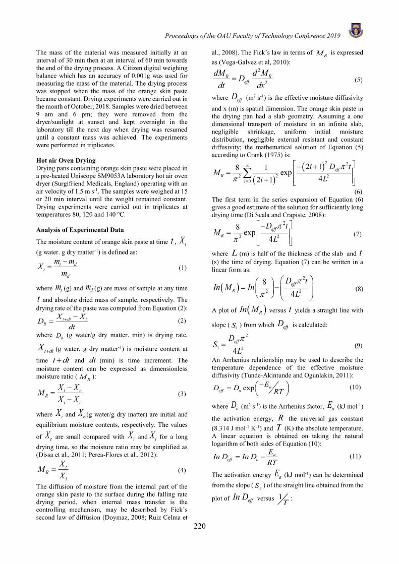
Proceedings of the OAU Faculty of Technology Conference 2019
220
The mass of the material was measured initially at an interval of 30 min then at an interval of 60 min towards the end of the drying process. A Citizen digital weighing balance which has an accuracy of 0.001g was used for measuring the mass of the material. The drying process was stopped when the mass of the orange skin paste became constant. Drying experiments were carried out in the month of October, 2018. Samples were dried between 9 am and 6 pm; they were removed from the dryer/sunlight at sunset and kept overnight in the laboratory till the next day when drying was resumed until a constant mass was achieved. The experiments were performed in triplicates. Hot air Oven Drying Drying pans containing orange skin paste were placed in a pre-heated Uniscope SM9053A laboratory hot air oven dryer (Surgifriend Medicals, England) operating with an air velocity of 1.5 m s-1. The samples were weighed at 15 or 20 min interval until the weight remained constant. Drying experiments were carried out in triplicates at temperatures 80, 120 and 140 oC. Analysis of Experimental Data
The moisture content of orange skin paste at time t , tX (g water. g dry matter-1) is defined as:
t dt
d
m mXm−
= (1)
where tm (g) and dm (g) are mass of sample at any time
t and absolute dried mass of sample, respectively. The drying rate of the paste was computed from Equation (2):
t dt tR
X XDdt
+ −= (2)
where RD (g water/g dry matter. min) is drying rate,
t dtX + (g water. g dry matter-1) is moisture content at
time t dt+ and dt (min) is time increment. The moisture content can be expressed as dimensionless moisture ratio ( RM ):
t eR
i e
X XMX X
−=
− (3)
where iX and eX (g water/g dry matter) are initial and equilibrium moisture contents, respectively. The values
of eX are small compared with tX and iX for a long drying time, so the moisture ratio may be simplified as (Dissa et al., 2011; Perea-Flores et al., 2012):
tR
i
XMX
= (4)
The diffusion of moisture from the internal part of the orange skin paste to the surface during the falling rate drying period, when internal mass transfer is the controlling mechanism, may be described by Fick’s second law of diffusion (Doymaz, 2008; Ruiz Celma et
al., 2008). The Fick’s law in terms of RM is expressed as (Vega-Galvez et al, 2010):
2
2R R
effdM d MD
dt dx= (5)
where effD (m2 s-1) is the effective moisture diffusivity and x (m) is spatial dimension. The orange skin paste in the drying pan had a slab geometry. Assuming a one dimensional transport of moisture in an infinite slab, negligible shrinkage, uniform initial moisture distribution, negligible external resistant and constant diffusivity; the mathematical solution of Equation (5) according to Crank (1975) is:
( )( )2 2
22 20
2 18 1 exp42 1
effR
i
i D tM
Li
=
− +=
+
(6) The first term in the series expansion of Equation (6) gives a good estimate of the solution for sufficiently long drying time (Di Scala and Crapiste, 2008):
2
2 2
8 exp4
effR
D tM
L
−=
(7)
where L (m) is half of the thickness of the slab and t (s) the time of drying. Equation (7) can be written in a linear form as:
( )2
2 2
84eff
R
D tIn M In
L
= − (8)
A plot of ( )RIn M versus t yields a straight line with
slope ( 1S ) from which effD is calculated: 2
1 24effD
SL
= (9)
An Arrhenius relationship may be used to describe the temperature dependence of the effective moisture diffusivity (Tunde-Akintunde and Ogunlakin, 2011):
exp aeff o
ED D RT− =
(10)
where oD (m2 s-1) is the Arrhenius factor, aE (kJ mol-1)
the activation energy, R the universal gas constant (8.314 J mol-1 K-1) and T (K) the absolute temperature. A linear equation is obtained on taking the natural logarithm of both sides of Equation (10):
aeff o
EIn D In DRT
= − (11)
The activation energy aE (kJ mol-1) can be determined from the slope ( 2S ) of the straight line obtained from the
plot of effIn D versus 1T :
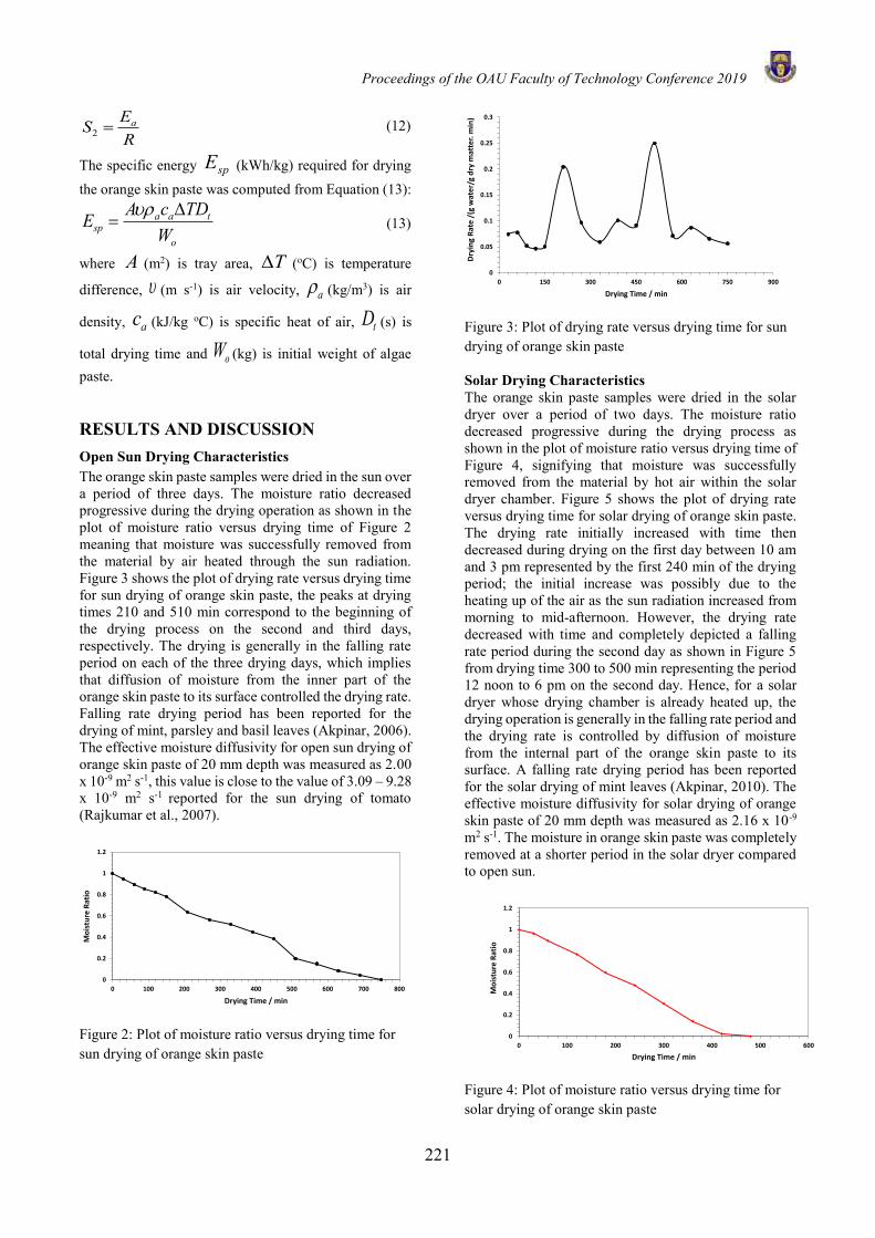
Proceedings of the OAU Faculty of Technology Conference 2019
221
2aES
R= (12)
The specific energy spE (kWh/kg) required for drying the orange skin paste was computed from Equation (13):
a a tsp
o
A c TDEW
= (13)
where A (m2) is tray area, T (oC)
is temperature
difference, (m s-1) is air velocity, a (kg/m3) is air
density, ac (kJ/kg oC) is specific heat of air, tD (s) is
total drying time and oW (kg) is initial weight of algae paste.
RESULTS AND DISCUSSION Open Sun Drying Characteristics The orange skin paste samples were dried in the sun over a period of three days. The moisture ratio decreased progressive during the drying operation as shown in the plot of moisture ratio versus drying time of Figure 2 meaning that moisture was successfully removed from the material by air heated through the sun radiation. Figure 3 shows the plot of drying rate versus drying time for sun drying of orange skin paste, the peaks at drying times 210 and 510 min correspond to the beginning of the drying process on the second and third days, respectively. The drying is generally in the falling rate period on each of the three drying days, which implies that diffusion of moisture from the inner part of the orange skin paste to its surface controlled the drying rate. Falling rate drying period has been reported for the drying of mint, parsley and basil leaves (Akpinar, 2006). The effective moisture diffusivity for open sun drying of orange skin paste of 20 mm depth was measured as 2.00 x 10⁻⁹ m2 s-1, this value is close to the value of 3.09 – 9.28 x 10⁻⁹ m2 s-1 reported for the sun drying of tomato (Rajkumar et al., 2007).
Figure 2: Plot of moisture ratio versus drying time for sun drying of orange skin paste
Figure 3: Plot of drying rate versus drying time for sun drying of orange skin paste
Solar Drying Characteristics The orange skin paste samples were dried in the solar dryer over a period of two days. The moisture ratio decreased progressive during the drying process as shown in the plot of moisture ratio versus drying time of Figure 4, signifying that moisture was successfully removed from the material by hot air within the solar dryer chamber. Figure 5 shows the plot of drying rate versus drying time for solar drying of orange skin paste. The drying rate initially increased with time then decreased during drying on the first day between 10 am and 3 pm represented by the first 240 min of the drying period; the initial increase was possibly due to the heating up of the air as the sun radiation increased from morning to mid-afternoon. However, the drying rate decreased with time and completely depicted a falling rate period during the second day as shown in Figure 5 from drying time 300 to 500 min representing the period 12 noon to 6 pm on the second day. Hence, for a solar dryer whose drying chamber is already heated up, the drying operation is generally in the falling rate period and the drying rate is controlled by diffusion of moisture from the internal part of the orange skin paste to its surface. A falling rate drying period has been reported for the solar drying of mint leaves (Akpinar, 2010). The effective moisture diffusivity for solar drying of orange skin paste of 20 mm depth was measured as 2.16 x 10⁻⁹ m2 s-1. The moisture in orange skin paste was completely removed at a shorter period in the solar dryer compared to open sun.
Figure 4: Plot of moisture ratio versus drying time for solar drying of orange skin paste
0
0.2
0.4
0.6
0.8
1
1.2
0 100 200 300 400 500 600 700 800
Mo
istu
re R
atio
Drying Time / min
0
0.05
0.1
0.15
0.2
0.25
0.3
0 150 300 450 600 750 900
Dry
ing
Rat
e /
(g w
ate
r/g
dry
ma
tte
r. m
in)
Drying Time / min
0
0.2
0.4
0.6
0.8
1
1.2
0 100 200 300 400 500 600
Mo
istu
re R
atio
Drying Time / min
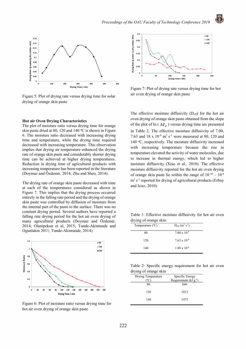
Proceedings of the OAU Faculty of Technology Conference 2019
222
Figure 5: Plot of drying rate versus drying time for solar drying of orange skin paste
Hot air Oven Drying Characteristics The plot of moisture ratio versus drying time for orange skin paste dried at 80, 120 and 140 oC is shown in Figure 6. The moisture ratio decreased with increasing drying time and temperature, while the drying time required decreased with increasing temperature. This observation implies that drying air temperature enhanced the drying rate of orange skin paste and considerably shorter drying time can be achieved at higher drying temperatures. Reduction in drying time of agricultural products with increasing temperature has been reported in the literature (Doymaz and Özdemir, 2014; Zhu and Shen, 2014). The drying rate of orange skin paste decreased with time at each of the temperatures considered as shown in Figure 7. This implies that the drying process occurred entirely in the falling rate period and the drying of orange skin paste was controlled by diffusion of moisture from the internal part of the paste to the surface. There was no constant drying period. Several authors have reported a falling rate drying period for the hot air oven drying of many agricultural products (Doymaz and Özdemir, 2014; Olanipekun et al, 2015; Tunde-Akintunde and Ogunlakin 2011; Tunde-Akintunde, 2014).
Figure 6: Plot of moisture ratio versus drying time for hot air oven drying of orange skin paste
Figure 7: Plot of drying rate versus drying time for hot air oven drying of orange skin paste
The effective moisture diffusivity (Deff) for the hot air oven drying of orange skin paste obtained from the slope of the plot of In ( RM ) versus drying time are presented in Table 2. The effective moisture diffusivity of 7.00, 7.63 and 18 x 10-9 m2 s-1 were measured at 80, 120 and 140 oC, respectively. The moisture diffusivity increased with increasing temperature because the rise in temperature elevated the activity of water molecules, due to increase in thermal energy, which led to higher moisture diffusivity (Xiao et al., 2010). The effective moisture diffusivity reported for the hot air oven drying of orange skin paste lie within the range of 10-10 – 10-8 m2 s-1 reported for drying of agricultural products (Erbay and Icier, 2010).
Table 1: Effective moisture diffusivity for hot air oven drying of orange skin
Temperature (oC) Deff (m2 s-1)
80 7.00 x 10⁻⁹
120 7.63 x 10⁻⁹
140 1.80 x 10⁻⁸
Table 2: Specific energy requirement for hot air oven drying of orange skin
Drying Temperature (oC)
Specific Energy Requirement (kJ g-1)
80 846
120 1013
140 1475
0
0.02
0.04
0.06
0.08
0.1
0.12
0.14
0.16
0.18
0 100 200 300 400 500 600
Dry
ing
Rat
e (
g w
ate
r/g
dry
mat
ter.
min
)
Drying Time / min
0
0.2
0.4
0.6
0.8
1
1.2
0 20 40 60 80 100 120 140 160 180 200 220 240
Mo
istu
re R
ati
o
Drying Time / min
80
120
140
0
0.05
0.1
0.15
0.2
0.25
0.3
0 50 100 150 200 250
Dry
ing
Rat
e (g
wat
er /
g d
ry m
atte
r. M
in)
Drying Time / Min
80
120
140
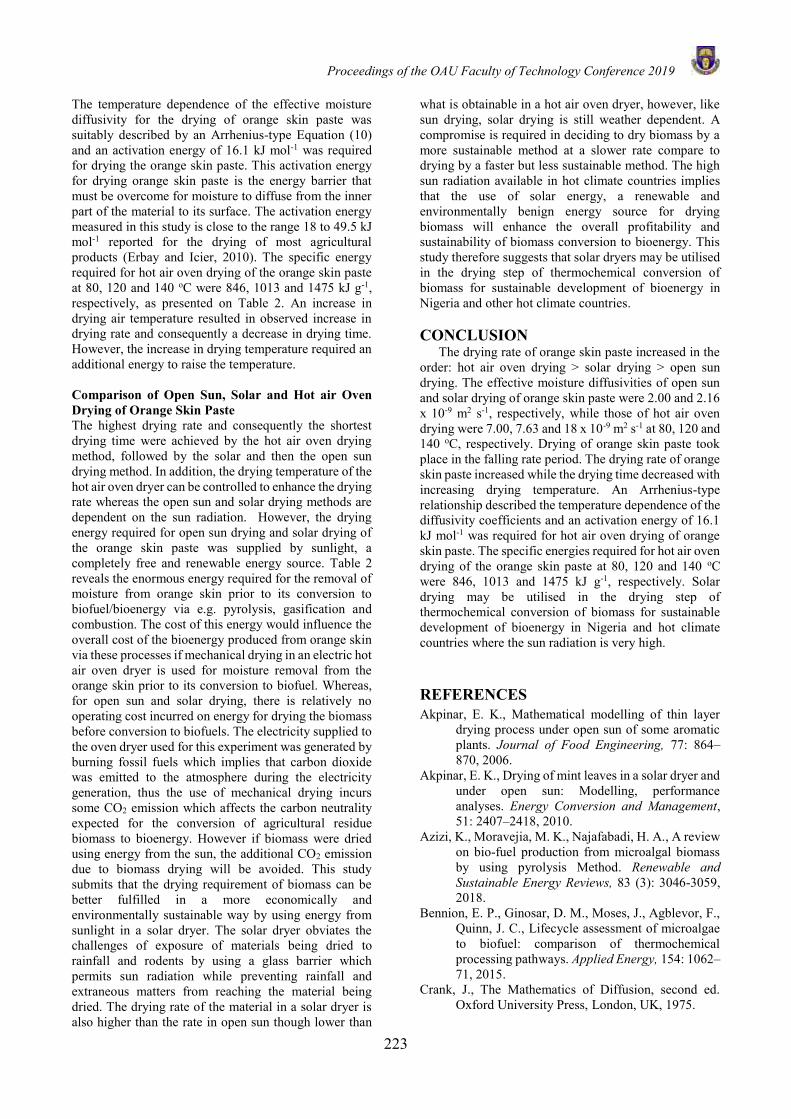
Proceedings of the OAU Faculty of Technology Conference 2019
223
The temperature dependence of the effective moisture diffusivity for the drying of orange skin paste was suitably described by an Arrhenius-type Equation (10) and an activation energy of 16.1 kJ mol-1 was required for drying the orange skin paste. This activation energy for drying orange skin paste is the energy barrier that must be overcome for moisture to diffuse from the inner part of the material to its surface. The activation energy measured in this study is close to the range 18 to 49.5 kJ mol-1 reported for the drying of most agricultural products (Erbay and Icier, 2010). The specific energy required for hot air oven drying of the orange skin paste at 80, 120 and 140 oC were 846, 1013 and 1475 kJ g-1, respectively, as presented on Table 2. An increase in drying air temperature resulted in observed increase in drying rate and consequently a decrease in drying time. However, the increase in drying temperature required an additional energy to raise the temperature. Comparison of Open Sun, Solar and Hot air Oven Drying of Orange Skin Paste The highest drying rate and consequently the shortest drying time were achieved by the hot air oven drying method, followed by the solar and then the open sun drying method. In addition, the drying temperature of the hot air oven dryer can be controlled to enhance the drying rate whereas the open sun and solar drying methods are dependent on the sun radiation. However, the drying energy required for open sun drying and solar drying of the orange skin paste was supplied by sunlight, a completely free and renewable energy source. Table 2 reveals the enormous energy required for the removal of moisture from orange skin prior to its conversion to biofuel/bioenergy via e.g. pyrolysis, gasification and combustion. The cost of this energy would influence the overall cost of the bioenergy produced from orange skin via these processes if mechanical drying in an electric hot air oven dryer is used for moisture removal from the orange skin prior to its conversion to biofuel. Whereas, for open sun and solar drying, there is relatively no operating cost incurred on energy for drying the biomass before conversion to biofuels. The electricity supplied to the oven dryer used for this experiment was generated by burning fossil fuels which implies that carbon dioxide was emitted to the atmosphere during the electricity generation, thus the use of mechanical drying incurs some CO2 emission which affects the carbon neutrality expected for the conversion of agricultural residue biomass to bioenergy. However if biomass were dried using energy from the sun, the additional CO2 emission due to biomass drying will be avoided. This study submits that the drying requirement of biomass can be better fulfilled in a more economically and environmentally sustainable way by using energy from sunlight in a solar dryer. The solar dryer obviates the challenges of exposure of materials being dried to rainfall and rodents by using a glass barrier which permits sun radiation while preventing rainfall and extraneous matters from reaching the material being dried. The drying rate of the material in a solar dryer is also higher than the rate in open sun though lower than
what is obtainable in a hot air oven dryer, however, like sun drying, solar drying is still weather dependent. A compromise is required in deciding to dry biomass by a more sustainable method at a slower rate compare to drying by a faster but less sustainable method. The high sun radiation available in hot climate countries implies that the use of solar energy, a renewable and environmentally benign energy source for drying biomass will enhance the overall profitability and sustainability of biomass conversion to bioenergy. This study therefore suggests that solar dryers may be utilised in the drying step of thermochemical conversion of biomass for sustainable development of bioenergy in Nigeria and other hot climate countries. CONCLUSION
The drying rate of orange skin paste increased in the order: hot air oven drying > solar drying > open sun drying. The effective moisture diffusivities of open sun and solar drying of orange skin paste were 2.00 and 2.16 x 10⁻⁹ m2 s-1, respectively, while those of hot air oven drying were 7.00, 7.63 and 18 x 10-9 m2 s-1 at 80, 120 and 140 oC, respectively. Drying of orange skin paste took place in the falling rate period. The drying rate of orange skin paste increased while the drying time decreased with increasing drying temperature. An Arrhenius-type relationship described the temperature dependence of the diffusivity coefficients and an activation energy of 16.1 kJ mol-1 was required for hot air oven drying of orange skin paste. The specific energies required for hot air oven drying of the orange skin paste at 80, 120 and 140 oC were 846, 1013 and 1475 kJ g-1, respectively. Solar drying may be utilised in the drying step of thermochemical conversion of biomass for sustainable development of bioenergy in Nigeria and hot climate countries where the sun radiation is very high. REFERENCES Akpinar, E. K., Mathematical modelling of thin layer
drying process under open sun of some aromatic plants. Journal of Food Engineering, 77: 864–870, 2006.
Akpinar, E. K., Drying of mint leaves in a solar dryer and under open sun: Modelling, performance analyses. Energy Conversion and Management, 51: 2407–2418, 2010.
Azizi, K., Moravejia, M. K., Najafabadi, H. A., A review on bio-fuel production from microalgal biomass by using pyrolysis Method. Renewable and Sustainable Energy Reviews, 83 (3): 3046-3059, 2018.
Bennion, E. P., Ginosar, D. M., Moses, J., Agblevor, F., Quinn, J. C., Lifecycle assessment of microalgae to biofuel: comparison of thermochemical processing pathways. Applied Energy, 154: 1062–71, 2015.
Crank, J., The Mathematics of Diffusion, second ed. Oxford University Press, London, UK, 1975.
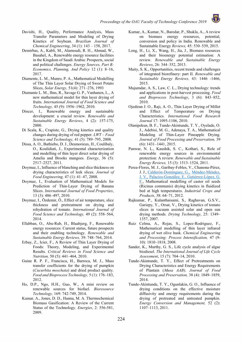
Proceedings of the OAU Faculty of Technology Conference 2019
224
Davishi, H., Quality, Performance Analysis, Mass Transfer Parameters and Modeling of Drying Kinetics of Soybean. Brazilian Journal of Chemical Engineering, 34 (1): 143 – 158, 2017.
Demirbas, A., Kabli, M., Alamoudi, R. H., Ahmad, W., Basahel, A., Renewable energy resource facilities in the Kingdom of Saudi Arabia: Prospects, social and political challenges. Energy Sources, Part B: Economics, Planning, And Policy 12 (1): 8–16, 2017.
Diamente, L. M., Munro, P. A., Mathematical Modelling of The Thin Layer Solar Drying of Sweet Potato Slices, Solar Energy, 51(4): 271–276, 1993
Diamante L. M., Ihns, R., Savage G. P., Vanhanen, L., A new mathematical model for thin layer drying of fruits. International Journal of Food Science and Technology, 45 (9): 1956–1962, 2010.
Dincer, I., Renewable energy and sustainable development: a crucial review. Renewable and Sustainable Energy Reviews, 4 (2): 157-175, 2000.
Di Scala, K., Crapiste, G., Drying kinetics and quality changes during drying of red pepper. LWT – Food Science and Technology, 41 (5): 789–795, 2008.
Dissa, A. O., Bathiebo, D. J., Desmorieux, H., Coulibaly, O., Koulidiati, J., Experimental characterization and modelling of thin layer direct solar drying of Amelia and Brooks mangoes. Energy, 36 (5): 2517–2527, 2011.
Doymaz, I., Influence of blanching and slice thickness on drying characteristics of leek slices. Journal of Food Engineering, 47 (1): 41–47, 2008.
Doymaz, I., Evaluation of Mathematical Models for Prediction of Thin-Layer Drying of Banana Slices. International Journal of Food Properties, 13 (3): 486–497, 2010.
Doymaz, I., Özdemir, Ö., Effect of air temperature, slice thickness and pretreatment on drying and rehydration of tomato. International Journal of Food Science and Technology, 49 (2): 558–564, 2014.
Ellabban, O., Abu-Rub, H., Blaabjerg, F., Renewable energy resources: Current status, future prospects and their enabling technology. Renewable and Sustainable Energy Reviews, 39: 748–764, 2014.
Erbay, Z., Icier, F., A Review of Thin Layer Drying of Foods: Theory, Modeling, and Experimental Results. Critical Reviews in Food Science and Nutrition, 50 (5): 441–464, 2010.
Guine R. P. F., Francisca, H., Barroca, M. J., Mass transfer coefficients for the drying of pumpkin (Cucurbita moschata) and dried product quality. Food and Bioprocess Technology, 5 (1): 176–183, 2012.
Ho, D.P., Ngo, H.H., Guo, W., A mini review on renewable sources for biofuel. Bioresource Technology, 169: 742-749, 2014.
Kumar, A., Jones, D. D., Hanna, M. A. Thermochemical Biomass Gasification: A Review of the Current Status of the Technology. Energies, 2: 556-581, 2009.
Kumar, A., Kumar, N., Baredar, P., Shukla, A., A review on biomass energy resources, potential, conversion and policy in India. Renewable and Sustainable Energy Reviews, 45: 530–539, 2015.
Long, H., Li, X., Wang, H., Jia, J., Biomass resources and their bioenergy potential estimation: A review. Renewable and Sustainable Energy Reviews, 26: 344–352, 2013.
Maity, S. K., Opportunities, recent trends and challenges of integrated biorefinery: part II. Renewable and Sustainable Energy Reviews, 43: 1446 -1466, 2015.
Mujumdar, A. S., Law, C. L., Drying technology: trends and applications in post-harvest processing. Food and Bioprocess Technology, 3 (6): 843–852, 2010.
Ojediran J. O., Raji, A. O., Thin Layer Drying of Millet and Effect of Temperature on Drying Characteristics. International Food Research Journal 17: 1095-1106, 2010.
Olanipekun, B. F., Tunde-Akintunde, T. Y., Oyelade, O. J., Adebisi, M. G., Adenaya, T. A., Mathematical Modeling of Thin-Layer Pineapple Drying. Journal of Food Processing and Preservation, 39 (6): 1431–1441, 2015.
Panwar, N. L., Kaushik, S. C., Kothari, S., Role of renewable energy sources in environmental protection: A review. Renewable and Sustainable Energy Reviews, 15 (3): 1513–1524, 2011.
Perea-Flores, M. J., Garibay-Febles, V., Chanona-Pérez, J. J., Calderón-Domínguez, G., Méndez-Méndez, J. V., Palacios-González, E., Gutiérrez-López, G. F., Mathematical modelling of castor oil seeds (Ricinus communis) drying kinetics in fluidized bed at high temperatures. Industrial Crops and Products, 38: 64–71, 2012.
Rajkumar, P., Kulanthaisami, S., Raghavan, G.S.V., Gariepy, Y., Orsat, V., Drying kinetics of tomato slices in vacuum assisted solar and open sun drying methods. Drying Technology, 25: 1349–1357, 2007.
Ruiz Celma, A., Rojas, S., Lopez-Rodriguez, F., Mathematical modelling of thin layer infrared drying of wet olive husk. Chemical Engineering and Processing: Process Intensification, 47 (9-10): 1810–1818, 2008.
Sander, K., Murthy, G. S., Life cycle analysis of algae biodiesel. The International Journal of Life Cycle Assessment, 15 (7): 704–14, 2010.
Tunde-Akintunde, T. Y., Effect of Pretreatments on Drying Characteristics and Energy Requirements of Plantain (Musa AAB). Journal of Food Processing and Preservation, 38 (4): 1849–1859, 2014.
Tunde-Akintunde, T. Y., Ogunlakin, G. O., Influence of drying conditions on the effective moisture diffusivity and energy requirements during the drying of pretreated and untreated pumpkin. Energy Conversion and Management, 52 (2): 1107–1113, 2011.

Proceedings of the OAU Faculty of Technology Conference 2019
225
Vega-Galvez, A., Miranda, M., Diaz, L. P., Lopez, L., Rodriguez, K., Di Scala, K., Effective moisture diffusivity determination and mathematical modelling of the drying curves of the olive-waste cake. Bioresource Technology, 101 (19): 7265–7270, 2010.
Xiao, H. W., Pang, C. L., Wang, L. H., Bai, J. W., Yang, W. X., Gao, Z. J., Drying kinetics and quality of Monukka seedless grapes dried in an air-impingement jet dryer. Biosystems Engineering, 105 (2): 233–240, 2010.
Zhu, A., Shen, X., The model and mass transfer characteristics of convection drying of peach slices. International Journal of Heat and Mass Transfer 72: 345–351, 2014.
Proceedings of the OAU Faculty of Technology Conference 2019
226
FUNCTIONAL AND PHYSICO-CHEMICAL PROPERTIES OF MALTED AMARANTH AND ROASTED SESAME FLOUR BLENDS: POTENTIAL
BREAKFAST MEAL BASE
A.V. Ikujenlola*, F.O. Ojedokun and S.H. Abiose Department of Food Science and Technology
Obafemi Awolowo University, Ile-Ife, Nigeria.
*Email of Corresponding Author: A.V. Ikujenlola; [email protected]
ABSTRACT Flour blends from malted amaranth and roasted sesame were evaluated for their functional, pasting and physicochemical properties. This was with a view to formulating a breakfast meal flour base that could replace wheat in production of breakfast cereals. Amaranth grains were cleaned, steeped, malted, dried, milled and packaged. The sesame seeds were roasted, milled, defatted, dried and packaged. The flour samples were blended in various ratios (100:0, 90:10, 80:20, 70:30 and 50:50 amaranth: sesame). Wheat flour served as the control. The flour blends were assessed for selected parameters following standard methods. The results showed that malting and addition of roasted sesame to amaranth improved the protein, ash, fat and crude fibre content of the flour blends. These parameters were significantly (p≤0.05) higher than that of the control. The values of water/oil absorption and swelling capacities, viscosity and bulk density decreased with the increase in the level of sesame substitution. The potassium ranged between 344.76 and 422.24mg/100g.The final viscosity ranged from 118.422 to 252.17RVU for malted samples. The study concluded that malting reduced the viscosity and bulk density of the flour blends while other parameters were increased. The inclusion of sesame to amaranth flour produced flour blends of higher nutritional quality. The blends have a potential to serve as a viable replacement in the production of breakfast cereal. Keywords: malting, pasting, roasting, viscosity, water capacity INTRODUCTION Breakfast cereals fall under two broad categories cereals that require namely: traditional and ready-to-eat cereals. Traditional cereals generally require further cooking or processing before consumption and are usually derived from oats, wheat, rice, sorghum, millet and corn. Ready-to-eat cereals may be classified into hot, whole-grain, bran, sugary and organic cereals depending on the production methods (Tribelhorn, 2009). Breakfast cereals formulated to provides-substantial amount of protein, calorie, fibre, iron, zinc, and vitamins in daily diets. Some common breakfast cereal products in Nigeria include: nasco cornflakes, good morning corn flakes, kellogg’s flakes, nabisco flakes, weetabix, quaker oats, rice crisps, and lots more. Most of these industrially produced breakfast cereals are based on wheat.
Wheat is considered nutritionally poor, as cereal proteins are deficient in essential amino acids such as lysine and threonine (Dhingra and Jood, 2001). It has been implicated for the incidence of celiac disease: a systemic immune‐mediated disorder caused by the ingestion of gluten‐containing grains (Lionetti et al., 2015). Also, the persistence rise in wheat import bills occasioned by inability of Nigeria to produce enough wheat for domestic use calls for alternative sourcing.
The Amaranthus genotype species are cultivated as “pseudo cereals” which produce cereal-like grains. It is rich in carbohydrates, proteins and fats, comparable or
even superior to cereals themselves (Toader and Roman, 2009). It is underexploited although awareness about its nutritional quality has directed attention to it full use. Amaranth is not genetically modified, it is rarely allergenic because of the absence of gluten and could be used in foods designed to reduce allergies in sensitive individuals, such as celiac disease patients (Berti, 2004).
Sesame seed (Sesamum indicum L.) is one of these unique healthy foods with multiple beneficial effects including anti-aging, anti-cancer, anti-oxidative activity, anti-hypertensive, modulation of lipid metabolism and lipid peroxidation, enhancement of liver function, immune-regulatory and anti-thrombosis properties (Martinchik, 2011).
Several efforts have been geared towards using composite flour based on cereal and legumes/oil seeds in the production of breakfast cereals/meals. However, there is scanty information on the utilization of amaranth and sesame blends as breakfast cereal/meal base. Therefore, the aim of this study is to evaluate the functional and physicochemical properties of the flour blends of amaranth and sesame for possible utilization as raw materials for breakfast cereal/meal production.
MATERIALS AND METHODS Materials The materials used for this study were amaranth grains (Amaranthus virides), defatted roasted sesame seeds

Proceedings of the OAU Faculty of Technology Conference 2019
227
(Sesamum indicum), and chemical reagents etc. Amaranth grains were purchased from central market, Ondo, Ondo State while sesame seeds were purchased from Makurdi, Benue State. The seeds were taken to Botany Department herbarium at Obafemi Awolowo University, Ile-Ife for identification. The chemical reagent used were of analytical grade. Methods Production of unmalted and malted amaranth flour samples The amaranth grains were cleaned and washed to remove dirt and stones. The grains were dried at 60 ºC for 10 hrs and winnowed. It was then milled, sieved and packaged in high-density polyethylene (HDPE). For malted amaranth flour, it was carried out using the method described by Gamel et al. (2006). Raw amaranth grains were cleaned and washed to remove dirt and stones. The cleaned grains were steeped in water at room temperature (30 ± 2 ºC) for 8 hrs and drained. The steeped grains were spread in a germinating chamber and watered twice a day for 48 hrs after which the sprouts were washed and dried in a cabinet dryer at 60 ºC for 20hrs. The dried grains were devegetated by rubbing the grains in between palms and the malted grains were milled, sieved and packaged in HDPE. Figure1 shows the flow diagram of the production of unmalted and malted amaranth flour. Production of roasted sesame flour Sesame seeds were cleaned to remove all the extraneous materials. Sesame seeds were roasted at 150 ºC for 5 mins until lightly brown. The roasted seeds were milled defatted, dried and packaged in high density polythene bag. The Fig.1 shows the flow chart for production of sesame flour samples. Sample Formulation and Analyses The amaranth (unmalted and malted) flour and roasted sesame flour were blended at various ratios of 100:0; 90:10; 80:20; 70:30; and 50:50 respectively. The blended samples were analysed for their proximate composition, functional, mineral and pasting characteristics. Proximate composition and functional properties determination The samples were analysed for moisture content, crude fat, crude protein, ash content, crude fibre, carbohydrate content based on the method of analysis of the Association of Official Analytical Chemists (AOAC, 2005). Bulk density was determined by the method of Okezie and Bello (1988). A 10 ml graduated cylinder was gently filled with the flours. The bottom of the cylinder was gently tapped on a laboratory bench several times until there was no further diminution of the sample level after filling to the 10 ml mark. Bulk density was calculated as weight of sample per unit volume of sample (g/ml).
Figure 1: Production of unmalted and malted amaranth flour and defatted roasted sesame flour Water absorption capacity was determined by the method of Onwuka (2005). Samples (1g, dry basis) were weighed into conical graduated centrifuge tubes of known weights and mixed with 10ml of distilled water for one minute with a glass rod. The tubes were made to undergo centrifugation at 5000 rpm for 30mins. The volume of supernatant was decanted and each tube together with its content reweighed as water absorbed per
Proceedings of the OAU Faculty of Technology Conference 2019
228
gram of sample. The difference in volume gave the water absorbed by 1g of the tested sample. Swelling capacity was determined using the method described by Akpata and Miachi (2001). One gram of the sample was weighed into centrifuge tube of known weight (2 cm in diameter) and 10 ml of distilled water was added and mixed gently using a glass stirring rod. The slurry formed was heated separately at a constant temperature (60, 70, 80, and 90°C) in a water bath for 15 min. During heating, the slurry was stirred with a glass rod gently to prevent clumping of the starch. At the end of 15 min, the tube containing the paste was centrifuged at 3000 × g for 30 min using a centrifuge (0502-1 Hospibrand, USA). The supernatant was decanted immediately after centrifugation. The tubes were dried at 50°C for 30 min, cooled and then weighed. Centrifuge tubes containing sample alone was weighed prior to adding distilled water. Swelling capacity was expressed as gram.
Pasting Characteristics Determination Pasting characteristics of blends was evaluated using a Rapid viscos analyser (Newport Scientific Pty Ltd. Warrie‐wood NSW, Australia). Flour slurry, containing 12% solids, was heated from 30 to 95°C at a rate of 2.5°C/min, held at 95°C for 15 min, and cooled at the same rate to 50°C (Chinma et al., 2013). The pasting performance was automatically recorded on the graduated sheet of the amylogram. The peak viscosity, trough viscosity, breakdown viscosity, final viscosity, setback viscosity, peak time, and pasting temperature were read off the amylograph.
STATISTICAL ANALYSIS All experiments were performed in triplicate. Data obtained were subjected to one‐way analysis of variance while Duncan's multiple range test was conducted to separate the means. These were achieved using the Statistical Package for the Social Scientists (SPSS) version 23.0).
Mineral Analysis The determination of selected mineral elements (Ca, Fe, Mg, K, Na, P, Pb) was carried out by Atomic Absorption Spectrophotometry method (AOAC, 2005). The sample 0.5 g was weighed into 75ml digestion flask and 5ml digestion mixture was added and left overnight in a hood. It was digested for 2 hrs at 150 ºC, then left to cool for 10 mins. About 3ml of 6M Hydrochloric acid was added and digested for another one and half-hours. It was cooled and 30ml of distilled water was added. The tube was vigorously stirred. A sample aliquot was then transferred to the Auto analyser (Technicon AAU model) for total mineral analysis at 420 nm. Absorption Spectrophotometer (Perkin Elmer, model 402) while sodium and potassium were determined by flame photometery. RESULTS AND DISCUSSION
Proximate and Energy Value of the Samples The proximate composition of the different flour samples is presented in Table 1. The values for crude protein of the flour samples ranged between 11.07–15.04 %. The crude protein content of the control was 11.07%. The malted amaranth had higher crude protein compared to unmalted amaranth sample. Malting improved protein content of samples. This observation is in agreement with the report of Dewar (2016) on the effect of malting on sorghum protein content. The protein content of samples from amaranth enriched with defatted roasted sesame flour were significantly higher (p≤0.05) than the control (100% whole wheat flour). Wheat contains gluten which is lacking in amaranth. However, the high level of protein in amaranth and sesame flour blends would be advantageous to the consumers of product from the blends. Sesame flour which is an edible, creamy and light brown powder from sesame seeds has high protein content (15-20%) with high levels of methionine and tryptophan (Dipasa, 2006). The crude fat content of the flour samples ranged between 1.08 and 8.66 %. There was significant difference (p ≤0.05) in the fat content of the samples and control (100% whole wheat). Enujiagha et al. (2004) explained the activities of lipolytic enzymes produced during the malting process might have degraded the lipid present in the malted samples to fatty acids and glycerol. Similarly, Fasasi et al. (2007) reported that the low fat content recorded in fermented and malted powder samples will help in increasing the shelf life of the samples by decreasing the chances of rancidity and will contribute to the low energy value of the sample. Incorporation of sesame led to significance increase (p ≤ 0.05) in fat content of samples. The ash content of the flour samples ranged from 1.21 to 3.70 %. There was significant increase (p ≤ 0.05) in ash content of enriched samples and the control. Malting improved the ash content of samples. This result showed that there was an increase in total ash content of samples as the amount of sesame incorporation into amaranth increased. Increase in ash content of enriched samples might be attributed to the high value of mineral content of the sesame (Nayar and Mehra, 2002). Ash is an indication of the minerals content in a food sample. The crude fibre contents of the flour varied between 1.22 to 3.76 % with 100 % whole wheat and 50 % amaranth: 50% roasted sesame having lowest and highest values respectively. There was an increase in fibre content of samples as the amount of sesame incorporation into malted amaranth increased. There was no significant difference (p<0.05) in fibre of flour. Dietary fibre helps to prevent constipation, bowel problems and piles, so the richer the food is in fibre, the better for the consumer. The moisture content of the samples ranged between 10.24 and 10.76 %. Storage stability of flour is enhanced when it’s moisture content is low, as low moisture content slows down biochemical dependent reactions
Proceedings of the OAU Faculty of Technology Conference 2019
229
and prevent the growth of mould (Onimawo and Akubor, 2012). The carbohydrate content of the samples ranged between 58.05 and 74.8 % with 100 % whole wheat having the highest and 50 % amaranth and 50 % roasted sesame having the lowest value. Carbohydrate content decreased with increase in proportion of sesame incorporation. The amount of calories in a quantity or volume of a food preparation is called Energy value of the food and is a good index for comparing the true value of different foods. Eating a nutritious breakfast will provide energy that will last throughout the morning and can also help control weight. Adequate energy is required for optimum development and growth; this will promote normal growth and prevent energy malnutrition. FAO/WHO (1993) recommends a range of 400 to 435 and 350 to 400 kcal/100g for men and women respectively. The energy value of the flour blends ranged between 353.44 and 381.77kcal/100g.The implication of this is that the product should meet the energy requirement of an average human. In general, protein, fat, ash and fibre content of the malted amaranths and roasted sesame flour blends were significantly (p≤0.05) higher than that of the control. This implied that the flour blends were of better nutritional quality. Functional Properties of Flour Samples Functional properties of a food material affect how it interacts with other food components and determines its application and end use. Therefore, food items with good functional properties can be easily incorporated into other foods and will yield good quality and acceptable end products. The functional properties (oil absorption capacity, OAC; water absorption capacity, WAC; and bulk density, BD) of the flour blends are presented in Table 2. The oil absorption capacity of the flour samples ranged from 1.55-2.02 g/g. The unmalted amaranth has better OAC than malted amaranth samples. It was also observed that increase in the roasted sesame content in the blends led to decrease in the OAC. This is an indication of the rate at which protein molecules binds fat in food formulation (Onimawo and Akubor, 2012). Water absorption capacity(WAC) shows the ability of a food product to associate with water under conditions when water is limiting such as dough’s and pastes (Akubor et al., 2013). The WAC of the flour samples ranged from 1.54 - 1.97 g/g. According to Osungbaro et al. (2010) processing factors such as fermentation and germination have been found to increase the ability of flour to absorb water. This property is a function of the availability of hydrophilic groups and capacity of gel formation of macro molecules (Gomez et al., 2008). It
was also observed that WAC of the samples decreases with increased concentration of roasted sesame. This might be due to an increasing concentration of hydrophobic molecules as protein content increase. Akubor et al. (2013) reported that African star apple kernel flour (ASAKF) had higher WAC (2.5 g/g) than wheat flour (1.3 g/g) which was associated to the probable presence of higher hydrophilic constituents in ASAKF than in wheat flour. The bulk density (BD) of the flour samples varied between 0.69-0.83 g/ml. The BD of the control samples was 0.81 g/ml. The BD of unmalted amaranth was higher than that of malted amaranth an observation which is in agreement with a previous report by Gernah et al., (2011) who reported unmalted maize flour to have higher bulk density (1.17 g/ml) than malted maize flour (0.86 g/ml). However, the BD of the samples decreased as a result of increase in roasted sesame content of the blends. Malted and unmalted amaranth flour samples have BD comparable to the control sample. The density of flour is important as it affects mixing, packaging, and transportation. Nutritionally, low bulk density is advantageous because it engenders consumption of more quantity of the lighter food item and this will translate into more nutrients for the consumer. Since increase in level of sesame substitution produced flour of comparable bulk density with the control; breakfast cereal based on amaranth and sesame should have similar bulk density with that produced from only wheat. Swelling capacity (SWC) increase with an increase in temperature (Figure 1). The higher SWC of the malted amaranth was expected as the swelling of starch granules leads to the disruption of intermolecular hydrogen bonds, thus allowing more water to enter and enlarge the granules (Gernah et al., 2011). The malted flours, whose starches had been dextrinized could not swell as much as the starch of the unmalted amaranth. When starch dispersion is heated, the swelling of granules and starch polymer solubilisation also occur. Starch solubility is considered as an indicator of the degree of molecule in starch dispersion after cooling (Moongngram et al., 2011). The swelling capacity of wheat flour increase with increase in temperature. Mineral Content of the Flour Samples The mineral composition of the flour samples is shown in Table 3. The calcium content of the flour samples ranged from 2.97 – 4.23 mg/100g. Sample containing 50% malted amaranth and 50 % roasted sesame had the highest value of calcium content (4.23 mg/100g) while unmalted amaranth had the lowest (2.97mg/100g). The calcium content of the control sample (0.98 mg/100g) was lower than those of other samples. The incorporation of sesame improved the calcium content of the samples. It has been reported that sesame seeds have significantly higher amount of calcium (Unal and Yalcin, 2008). Malting process improved the calcium content of malted amaranth (3.64 mg/100g) compared to unmalted amaranth (2.97 mg/100g).
Proceedings of the OAU Faculty of Technology Conference 2019
230
The iron content of the flour samples ranged between 0.29 and 0.38 mg/100g. The iron content of the control (0.87 mg/100g) was lower than those of all the samples. Iron is essential in the formation of protein haemoglobin, which carries oxygen throughout the body in the red blood cells and myoglobin, which transports oxygen in the muscles The magnesium content of the samples ranged from 24.48 to 32.56 mg/100g. Unmalted amaranth had the lowest magnesium content of 24.48 mg/100g while sample containing 50% malted amaranth and 50% roasted amaranth had the highest magnesium content 32.56 mg/100g. This result showed that there was an increase in magnesium content of samples from (20.15 – 25.57 mg/100g) as the amount of sesame incorporated into amaranth increased. This result is in agreement with the report of Alonso et al., 2001 on magnesium content of bread from composite flour of sesame and wheat with the value ranging from 170.30 mg/100g to 235.69 mg/100g. The potassium content ranged between 344 and 422 mg/100g with significant variations (p ≤ 0.05) among the samples. This study showed that potassium was the most abundant and this observation was similar to other findings like Oshodi et al. (1999) who reported potassium to be the most abundant mineral in Nigerian Agricultural products. Sodium content of the flour samples ranged from 30.63 to 54.13 mg/100g. Sample 7 (whole wheat) has the lowest value and sample 6 has the highest sodium content. The body needs a small amount of sodium to help maintain normal blood pressure and normal function of muscles and nerves. It promotes healthy cell development and regulation. Phosphorus content of the flour samples ranged from 109.74 to 136.24 mg/100g. Phosphorus improve digestion, help in bone formation, improve energy extraction, optimize chemical reactions and proper utilization (Heaney et al., 2006). Lead was not detected in the samples. In general, the breakfast cereal base from amaranth blended with defatted roasted sesame had improved mineral levels and compared favourably with the control. Pasting Properties of Flour Samples Pasting properties is essential in categorizing the end-product application of flour. Table 4 summarizes the pasting properties of the various flour samples. This functionality is said to be dependent upon factors such as granule size, amylose/amylopectin ratio and starch property (Simi and Abraham, 2008). When starch-based foods are heated in an aqueous environment, they undergo series of changes known as gelatinization and pasting. These are two of the most important properties that influence quality and aesthetic considerations in the
food industry, since they affect texture and digestibility as well as the end use of starchy foods (Adebowale et al., 2005). Peak viscosity ranged from 20.83 to 66.67 RVU. The relative high peak viscosity of sample containing 100 % unmalted amaranth might be related to the proportion of starch in the unmalted sample, the ratio of amylose to amylopectin and the resistance of the starch granules to swelling (Jideani and Jideani, 2011). The presence of other non-starchy constituents in the other samples may be a contributing factor to the low peak viscosity observed. Low peak viscosities of the formulated samples implied that the samples will form a low viscous pastes rather than a thick gel on cooking and cooling (Adebowale et al., 2005). This will amount to use of more solid which will encourage more nutrients. The 100% unmalted amaranth sample had the highest trough value of 62.42RVU and sample containing 50% malted amaranth and 50 % roasted sesame had the lowest value of 27.25 RVU. The control had the highest trough value of 106.42 RVU of all the samples. Trough viscosity is the minimum viscosity value in the constant temperature phase of Rapid visco analysis profile and measures the ability of paste to withstand breakdown during cooling. Trough and breakdown viscosities are pasting properties which indicate the ability of a food material to remain undisrupted when subjected to long periods of constant high temperature and its ability to withstand breakdown during cooking (Normita and Cruz, 2002). The breakdown viscosity ranged from 2.58 to 5.42 RVU. The 100% unmalted amaranth had the highest breakdown viscosity (5.41 RVU) while sample containing 50% malted amaranth and 50 % roasted sesame had the lowest (2.58 RVU). The breakdown viscosity of the control was 22.08 RVU. The break down viscosity value is an index of stability of starch (Fernandez and Berry, 1989). The higher the breakdown viscosity, the lower the ability of sample to withstand heating and shearing stress during cooking (Adebowale et al., 2005). A higher pasting temperature implies higher water binding capacity, higher gelatinization and lower swelling property of starch due to a high degree of association between starch granules (Oluwamukomi et al., 2005). The pasting temperatures for flour samples ranged from 90.17 to 92.05 °C; lower than the pasting temperature of the control sample (95.43 °C). The pasting temperatures values of the samples were higher than the gelatinization temperature of 70.5 °C reported for Ogi (fermented corn) flour by Oluwamukomi et al., (2005) and Ohizua et al., (2017). In general, the control sample displayed higher values for peak, trough and breakdown viscosities. CONCLUSION

Proceedings of the OAU Faculty of Technology Conference 2019
231
This study elicited that incorporation of roasted sesame to malted amaranth flour samples improved the proximate and mineral compositions. Similarly, the functional and pasting characteristics of the amaranth based flours samples compared favourably with that of the control (wheat) sample. The study therefore
concluded that the flour blends from malted amaranth and roasted sesame have a potential to serve as a good replacement to wheat in the manufacture of breakfast cereal of high nutritional and physical qualities.
Table 1: Proximate composition of Amaranth and Sesame Flour Blends (%)
Samples Crude Protein
Crude Fat Total Ash Crude Fibre
Moisture Carbohydrate Energy (kcal/100g)
1 11.34±0.01f 7.77±0.02e 1.84±0.01f 2.34±0.01d 10.24±0.02g 66.47±0.02b 381.17±0.01a
2 11.55±0.01e 7.67±0.02f 3.34±0.02e 2.54±0.01c 10.35±0.01d 64.55±0.07c 373.43±0.01c
3 12.14±0.01d 8.06±0.01d 3.43±0.01d 2.58±0.01c 10.37±0.01e 63.42±0.01d 374.78±0.01b
4 13.34±0.01c 8.11±0.01c 3.51±0.01b 2.62±0.01b 10.46±0.01d 61.96±0.01e 374.19±0.01c
5 13.87±0.02b 8.23±0.01b 3.47±0.01c 2.65±0.01b 10.65±0.02b 61.13±0.01f 374.07±0.01c
6 15.04±0.01a 8.66±0.01a 3.73±0.01a 3.76±0.02a 10.76±0.01a 58.05±0.01g 361.75±0.01d
7 11.07±0.02g 1.08±0.01g 1.21±0.01g 1.22±0.02e 10.56±0.01c 74.86±0.01a 353.44±0.01e
Values with different Superscript on the same column are significant; Sample 1= 100%Unmalted Amaranth; Sample 2= 100% Malted Amaranth; Sample 3= 90% Malted Amaranth: 10% Roasted Sesame; Sample 4= 80% Malted Amaranth: 20% Roasted Sesame; Sample 5= 70% Malted Amaranth: 30% Roasted Sesame; Sample 6= 50% Malted Amaranth: 50% Roasted Sesame; Sample 7= 100% Whole Wheat Flour.
Table 2: Functional Properties of Amaranth and Sesame Flour Blends
Samples Oil Absorption Water Absorption Bulk Density
1 1.93±0.01b 1.61±0.01d 0.83±0.00a
2 2.02±0.03a 1.97±0.01a 0.80±0.01a
3 1.91±0.01b 1.73±0.02b 0.76±0.01b
4 1.82±0.02c 1.69±0.01c 0.74±0.01c
5 1.72±0.01d 1.63±0.02d 0.72±0.01d
6 1.55±0.01e 1.54±0.02e 0.69±0.01e
7 1.75±0.01d 1.52±0.01e 0.81±0.01a
Values with different Superscript on the same column are significant; Sample 1= 100% Unmalted Amaranth; Sample 2= 100% Malted Amaranth; Sample 3= 90% Malted Amaranth: 10% Roasted Sesame; Sample 4= 80% Malted Amaranth: 20% Roasted Sesame; Sample 5= 70% Malted Amaranth: 30% Roasted Sesame; Sample 6= 50 % Malted Amaranth: 50% Roasted Sesame; Sample 7= 100% Whole
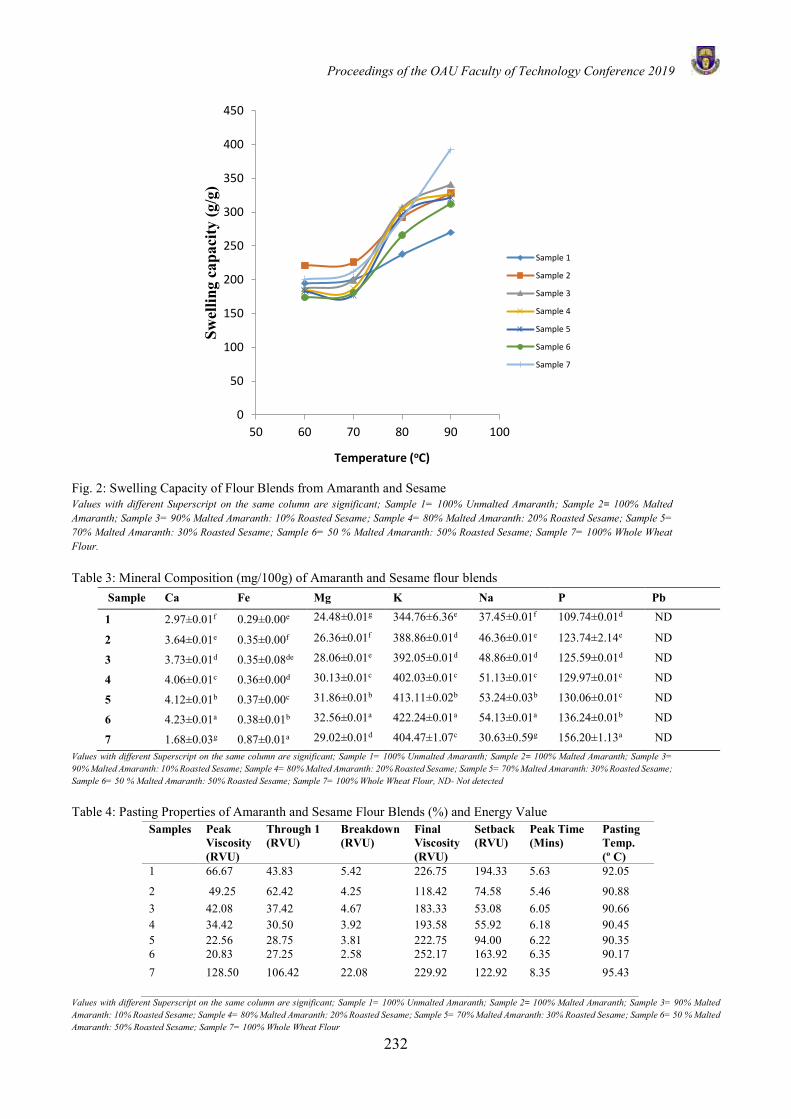
Proceedings of the OAU Faculty of Technology Conference 2019
232
Fig. 2: Swelling Capacity of Flour Blends from Amaranth and Sesame Values with different Superscript on the same column are significant; Sample 1= 100% Unmalted Amaranth; Sample 2= 100% Malted Amaranth; Sample 3= 90% Malted Amaranth: 10% Roasted Sesame; Sample 4= 80% Malted Amaranth: 20% Roasted Sesame; Sample 5= 70% Malted Amaranth: 30% Roasted Sesame; Sample 6= 50 % Malted Amaranth: 50% Roasted Sesame; Sample 7= 100% Whole Wheat Flour. Table 3: Mineral Composition (mg/100g) of Amaranth and Sesame flour blends
Sample Ca Fe Mg K Na P Pb
1 2.97±0.01f 0.29±0.00e 24.48±0.01g 344.76±6.36e 37.45±0.01f 109.74±0.01d ND
2 3.64±0.01e 0.35±0.00f 26.36±0.01f 388.86±0.01d 46.36±0.01e 123.74±2.14e ND
3 3.73±0.01d 0.35±0.08de 28.06±0.01e 392.05±0.01d 48.86±0.01d 125.59±0.01d ND
4 4.06±0.01c 0.36±0.00d 30.13±0.01c 402.03±0.01c 51.13±0.01c 129.97±0.01c ND
5 4.12±0.01b 0.37±0.00c 31.86±0.01b 413.11±0.02b 53.24±0.03b 130.06±0.01c ND
6 4.23±0.01a 0.38±0.01b 32.56±0.01a 422.24±0.01a 54.13±0.01a 136.24±0.01b ND
7 1.68±0.03g 0.87±0.01a 29.02±0.01d 404.47±1.07c 30.63±0.59g 156.20±1.13a ND
Values with different Superscript on the same column are significant; Sample 1= 100% Unmalted Amaranth; Sample 2= 100% Malted Amaranth; Sample 3= 90% Malted Amaranth: 10% Roasted Sesame; Sample 4= 80% Malted Amaranth: 20% Roasted Sesame; Sample 5= 70% Malted Amaranth: 30% Roasted Sesame; Sample 6= 50 % Malted Amaranth: 50% Roasted Sesame; Sample 7= 100% Whole Wheat Flour, ND- Not detected Table 4: Pasting Properties of Amaranth and Sesame Flour Blends (%) and Energy Value
Samples Peak Viscosity (RVU)
Through 1 (RVU)
Breakdown (RVU)
Final Viscosity (RVU)
Setback (RVU)
Peak Time (Mins)
Pasting Temp. (º C)
1 66.67 43.83 5.42 226.75 194.33 5.63 92.05
2 49.25 62.42 4.25 118.42 74.58 5.46 90.88 3 42.08 37.42 4.67 183.33 53.08 6.05 90.66 4 34.42 30.50 3.92 193.58 55.92 6.18 90.45 5 22.56 28.75 3.81 222.75 94.00 6.22 90.35 6 20.83 27.25 2.58 252.17 163.92 6.35 90.17 7 128.50 106.42 22.08 229.92 122.92 8.35 95.43
Values with different Superscript on the same column are significant; Sample 1= 100% Unmalted Amaranth; Sample 2= 100% Malted Amaranth; Sample 3= 90% Malted Amaranth: 10% Roasted Sesame; Sample 4= 80% Malted Amaranth: 20% Roasted Sesame; Sample 5= 70% Malted Amaranth: 30% Roasted Sesame; Sample 6= 50 % Malted Amaranth: 50% Roasted Sesame; Sample 7= 100% Whole Wheat Flour
0
50
100
150
200
250
300
350
400
450
50 60 70 80 90 100
Swel
ling
capa
city
(g/g
)
Temperature (oC)
Sample 1
Sample 2
Sample 3
Sample 4
Sample 5
Sample 6
Sample 7
Proceedings of the OAU Faculty of Technology Conference 2019
233
REFERENCES Akpata M. I., and Miachi O. E., “Proximate composition and
selected functional properties of Detarium microcarpum” Plant Foods for Human Nutrition, 56:297–302, 2001
Akubor, P. I., Yusuf, D. and Obiegunam, J. E. “Proximate composition and some functional properties of flour from the kernel of African star apple (Chrysophyllual albidium)” International Journal of Agricultural Policy and Research 1(3), 062-066, 2013.
AOAC. Official Methods of Analysis Association of Official Analytical Chemist. 16th edition Washington, DC: Association of Official Analytical Chemists, Inc, 2005.
Chinma C. E., Gbadamosi K. B., Ogunsina B. S., Oloyede O. O., and Salami S. O. “Effect of addition of germinated moringa seed flour on the quality attributes of wheat‐based cake” Journal of Food Processing and Preservation, 12(1), 3–6, 2013.
Dewar, J. Influence of Malting on Sorghum Protein Quality. www.afripro.org.uk. dietary_ guidelines. 2016. (Accessed 12th March 2017)
Dhingra, S. and Jood, S. Organoleptic and Nutritional Evaluation of Wheat Breads Supplemented with Soybean and Barley flour. Journal of Food Chemistry 77, 479-488, 2001.
Dipasa, B. M. Sesame honey bits. www.dipasa.nl/seshobit.htm.3-9 Accessed 12th March 2017, 2006.
Enujiugha, V. N., Thani, F. A., Sanni, T. M. and Abigor, R. D. “Lipase activity in dormant seeds of the african oil bean (Pentaclethra macrophylla Benth)” Food Chemistry, 88(3):405-415, 2004.
Fasasi, O. S., Eleyinmi, A. F. and Oyerekua, M. A. Effect of some traditional processing operations on the functional properties of african breadfruit seed (Treculia Africana) flour. Journal Food Science and Technology, 40, 513-519, 2007.
FAO/WHO Amino acid requirements of human ‘WHO’ technical report servious, energy and protein requirements for FAO/WHO nutrition reports series, 52,15-30,1993.
Gamel T. H, Lissen J. P, Messalleem A. S and Shekib L. A. Effect of seed treatments on the chemical composition of two amaranth species: oil, sugars, fibres, minerals and vitamins. Journal of the science of Food and Agriculture, 86, 82 -89, 2006.
Gernah, D. I., Ariahu, C. C., Ingbian, E. K. Effects of malting and fermentation on some chemical and functional properties of maize (Zea mays). America Journal of Food technology 6 (5), 404-412, 2011.
Hasmadi, M., Siti Faridah, A., Salwa,I., Matanjun,P., Abdul Hamid,M.and Rameli, A.S. The effect of sea weed composite flour on the textural properties of dough and bread. Journal of Applied Phycology 26:1057-1062, 2014.
Martinchik, A. N. “Nutritional value of sesame seeds” Journal Voprspitan 80:41-43, 2011.
Moongngram A., Paseephol T. and Phattanakulkaewmorie N. Chemical composition and physico-chemical properties of malted sorghum flour and characteristics of gluten free bread. World Academy of Science, Engineering and Technology pp 57-60, 2011.
Normita, M. and Cruz, R. D. “Rice grain quality evaluation procedure” International Rice Research Institute Discussion Paper Series No. 44 losbanos, Phillippines, 2002.
Ohizua E. R., Adeola A. A., Idowu M. A., Sobukola O. P., Afolabi T. A., Ishola R. O., Falomo A. “Nutrient composition, functional and pasting properties of unripe cooking banana, pigeon pea and sweet potato flour blend” Food Sciences and Nutrition, 5: 750–762, 2017.
Olapade A. A., and Oluwole O. B. Bread making potential of composite flour of wheat‐Acha enriched with cowpea flour. Nigerian Food Journal, 31(1), 6–12, 2013.
Onimawo, I. A. and Akubor, P. I. Food chemistry (Integrated Approach with Biochemical Background). 2nd edn. Joytal printing press, Agowo, Ibadan, Nigeria, 2012.
Onwuka, G. I. Food Analysis and Instrumentation (Theory and Practice) Napthala Prints, Surulere, Lagos, Nigeria. pp 140-160, 2005.
Oluwamukomi, M. O., Eleyinmi, A. F. and Enujiugha, V. M. “Effect of soy supplementation and its stage of inclusion on the quality of ogi- a fermented maize meal” Food chemistry, 55(1):1-6, 2005.
Oshodi, A. J. L., Ogungenle, H. N. and Oladimeji, N. O. Chemical composition, nutritionally valuable minerals and functional properties of benni seed (Sesanum Rediatum), Pearl Millet (Perntiisetimtyphoides) And Quinoa (Chenopodium Quinoa) Flours. International Journal of Food Science and Nutrition, 50: 325-331, 1999.
Osungbaro, T. O., Jimoh, D. and Osundeyi, E.”Functional and pasting properties of composite cassava-sorghum meals.”Agriculture and Biology Journal of North America, 24(2): 91-99, 2010.
Simi, C.K and Abraham T.E “Physicochemical rheological and thermal properties of rice (Oryza sativa) starch” Journal of Agriculture and Food Chemistry, 56, 12105-12113, 2008.
Toader, M. and Roman, G. V. “Experimental results regarding
morphological, biological and yield quality of amaranthus hypocondriacus L. species under the central part of romanian plain conditions” Reserves Journal of Agricultural Science and Nutrition, 41(1):54-57, 2009.
Tribelhorn R. E. Breakfast cereals. Handbook of Cereal
Science and Technology (Lorenz K. J and Kulp K. Eds), 741-762, Marcel Dekker Incorporated: New York, 2009.
Unal, M.K. and H. Yalcin” Proximate composition of Turkish
sesame seeds and characterization of their oils” Grasas Aceites, 59, 23-26, 2008.
Proceedings of the OAU Faculty of Technology Conference 2019
234
INFLUENCE OF WATER-CEMENT RATIO AND WATER REDUCING ADMIXTURES ON THE REBOUND NUMBER OF HARDENED CONCRETE
K. A. Olonade1,*, O. J. Oyebo2 and Y. O. Sulaiman2 1Department of Civil and Environmental Engineering,
University of Lagos, Akoka, Nigeria. 2Department of Civil Engineering,
Obafemi Awolowo University, Ile-Ife, Nigeria
*Email of Corresponding Author: [email protected]
ABSTRACT In this paper, effects of water-cement ratio and type of water reducing admixtures (WRA) on the Schmidt hammer rebound number (RN) were investigated. Concrete of mix ratio 1:2:4 was prepared at the w/c of 0.45. 0.50, 0.55 and 0.60 and with each of the three WRA at the w/c of 0.45. Concrete cubes of size 150 mm were cast and cured in water for 3, 7 and 28 days. RNs of the cubes were determined and the compressive strengths (fc) corresponding to the RNs obtained from the conversion graph supplied by the manufacturer were compared with the compressive strengths obtained from crushing machine (CM). The results showed that as the w/c increased, the RN increased up to when w/c was 0.5 and began to drop, while there was no significant effect of all the WRA on the RN. It was also found that fc obtained from CM and those obtained using the conversion graph differed considerably. A new correlation graph was therefore proposed, which showed a correlation coefficient of 0.96, while coefficient of determination obtained for the regression equation between RN and fc was as high as 0.92. The study concluded that w/c had effect on RN of SH and that the equation developed could be used to determine fc, once RN is known. Keywords: Rebound number, water-reducing admixture, compressive strength, water-cement ratio, correlation INTRODUCTION The frequency at which concrete structures collapse in most developing countries, especially Nigeria, has been a major concern for all stakeholders. In order to forestall a repeat of such preventable disasters, most old concrete structures are subjected to structural integrity assessment to be able to determine their fitness for use. In another situation, when additional storey is to be put on an existing building, there is always need to ascertain the capability of the existing structure to carry or accommodate the new storey. Also, where a concrete structure has been abandoned for a long period of time and there is need to resume construction, structural integrity of the structure would be required to determine its residual strength. It could also be required as routine check for the purpose of maintenance. Similarly, it could be deployed to settle rifts between contractors and consultants over quality of concrete used. In any of these cases, non-destructive testing (NDT) remains the major technique to adopt. Originally, NDT was developed for inspection of metals and pipelines to identify defects in steel. With this application, recognized national and international standards have been developed. Its use in concrete inspection was lately developed due to heterogeneous nature of concrete with varying constituents (Malhotra & Carino, 2004). In the recent past, quite a number of techniques have been developed to monitor concrete performance. Of these techniques, Rebound Hammer (RH) otherwise
known as Schmidt Hammer (SH) becomes more popular due to its simplicity of use and possibly less cost (Zaky, 2001). There are different types of SH that have been developed, depending on the impact energy. Common ones are L and N types, but there is no clear guidelines on what determine the choice of the type to use. While some standards specify a particular type of SH for use, quite a number of them did not specify hammer type, indicating that the type of hammer may not influence the results (Woodson, 2009). This technique, SH, measures the rebound number that is observed, when the plunger is pushed against a hard surface (ASTM C805-13, 2013). The rebound number (RN) measured could be a good representation of compressive strength of concrete, if sizeable numbers of points are measured in a grid (Woodson, 2009). Now, national and international standards have been developed for its use (ASTM C805-13, 2013; BS EN 12504-2, 2013; IS 13311 (Part 2), 2004) A considerable amount of literature has been published on the practical use of SH. These studies seem to assess the reliability of SH for determining in-place concrete quality, when compared with the traditional method of crushing test. Sanchez and Tarranza (2014) used SH to assess compressive strength of existing structure and compared their results with crushing test; it was found that SH test was comparable to crushing test. In a similar study conducted by Rubene and Vilnitis (2014) on series of laboratory tests, the compressive strength obtained from SH was marginally higher than that of crushing test by about 1.6%, which shows a high level of reliability of the
Proceedings of the OAU Faculty of Technology Conference 2019
235
technique. Strengths obtained from SH and Ultrasonic Pulse Velocity (UPV) were also found to be comparable to what was obtained from crushing test. However, combining the SH and UPV tests would give more accurate estimation of compressive strength of in-place concrete (Shariati, Ramli-Sulong, Arabnejad, Shafigh, & Sinaei, 2011). Brozovsky (2012) also monitored the strength of brick, using SH and obtained fairly reliable results, while Tamil et al. (2014) employed the technique to monitor strength development of concrete containing copper slag (CS) as fine aggregate. The results indicated that SH technique mirrors the strength development as CS content varied, when compared with crushing method. Apart from using SH in testing concrete quality, the method is also being used extensively to determine uniaxial strength of rock (Cargill & Shakoor, 1990). It has also been used as dating tool in archeological sciences (Frauenfelder, Laustela, & Kääb, 2005). One major challenge with the use of SH is finding appropriate correlation that will convert RN obtained from SH to compressive strength. Though, the manufacturer of SH often provides conversion curves, yet there have been strong criticisms as to the extent the curve can mimic all the factors affecting concrete strength. This is recognized by ASTM C805 (2013), when it recommends that users should develop a correlation for the device used on the concrete mixture to be tested, for more reliable results. Another limitation of the correlation given by the manufacturer is that surfaces that have low RN could not be used to estimate strength. This is because the relationship between hardness and concrete strength depends on factors affecting the concrete surface such as saturation degree, temperature, carbonation, surface preparation and direction of testing (Amasaki, 1991). Other factors that have been identified to have influence on the SH test include size of the specimen (Mitchell & Hoagland, 1961), aggregate type (Grieb, 1958), type of cement (Kolek, 1958). In similar trend, Yasar and Erdogan (2004) showed that SH rebound number reduced with increase in porosity and they developed an empirical equation, while Aydin and Basu (2005) established a correlation between RN and density of the material. Despite extensive literature on the role water-cement ratio (w/c) and chemical admixtures play on the mechanical and durability properties of concrete, the effect of both on the RN of SH of hardened concrete is still very unclear. In this study, therefore, attempt was made to establish influence of w/c and selected WRA on the RN of SH. An empirical function between the RN and w/c was developed, while correlation between the strength determined from SH and crushing test was equally established. The findings from this study should make an important contribution to the field of NDT. MATERIALS AND METHODS Materials The cement used for this research work was Elephant Lafarge cement acquired from a retail shop at Lagere,
Ile-Ife Osun State Nigeria. Sand of maximum nominal size of 3.35 mm and granite of maximum size of 18 mm were used as fine and coarse aggregates, respectively. Potable water was used for mixing, while WRAs used were plasticizers of brand names Rheobuild 850 and Mapaei NS100 and a superplasticizer, Meflux 101F. Concrete Mixing and Casting Concrete specimen used was batched by weight with mix ratio of 1:2:4 (cement: sand: granite) and varied water cement ratio at with dosage of superplasticizer. For assessing effect of w/c, different w/c ranging from 0.45 to 0.60 at intervals of 0.05 were studied, without WRAs. In the other concrete specimens, different WRAs were used at constant w/c of 0.45. Each WRAs was added to the concrete mix separately at average dosage recommended by their manufacturers. Specifically, the dosage used for every 50 kg of cement was 425.53 ml of Rheobuild, 531.91 ml of Mapaei NS100 and 262.5 g of Meflux 101F. The choice of fixed w/c of 0.45 was based preliminary study. In all, seven different concrete specimens were produced (S1 to S7). For instance, S1 was made with w/c of 0.45 without WRA, while S6 was made with w/c of 0.45 and Mapaei NS100. Prior to casting the concrete specimens into steel moulds of sizes 150 x 150 x 150 mm, slump test was carried out on the fresh concrete. Finally, six concrete cubes were cast for each concrete specimen, three samples each for SH test and crushing test. The moulds and their contents were covered with polythene bags to prevent loss of moisture for 24 hours. Thereafter, the concrete cubes were removed from the moulds and immersed in water for curing until the test dates of 3, 7 and 28 days. Methods Material characterization Chemical composition of the cement was determined using XRF, while its physical properties such as specific gravity (sg) and those of the aggregates were determined along with sieve analysis based on the provisions of BS EN 1097-3 (1998). Particle size distribution curves were plotted and grading coefficients (coefficients of curvature, Cc and uniformity, Cu) determined based on the equations provided by Peck et al. (1974) and reproduced here as Equations (1) and (2).
𝐶𝑢 = 𝐷10/𝐷60 (1)
𝐶𝑐 = (𝐷30)2/(𝐷10 𝑥 𝐷60) (2)
Where D10, D30 and D60 are diameters of the soil particle for which, 10, 30 and 60 percent of the particles are finer, respectively
Slump, Compressive strength and SH Rebound Number The only workability test performed on the fresh concrete mixes was slump test. This test was carried out according to BS EN 12350 (2009). As earlier mentioned, three cube samples from each concrete specimen were tested for compressive strength using crushing method in
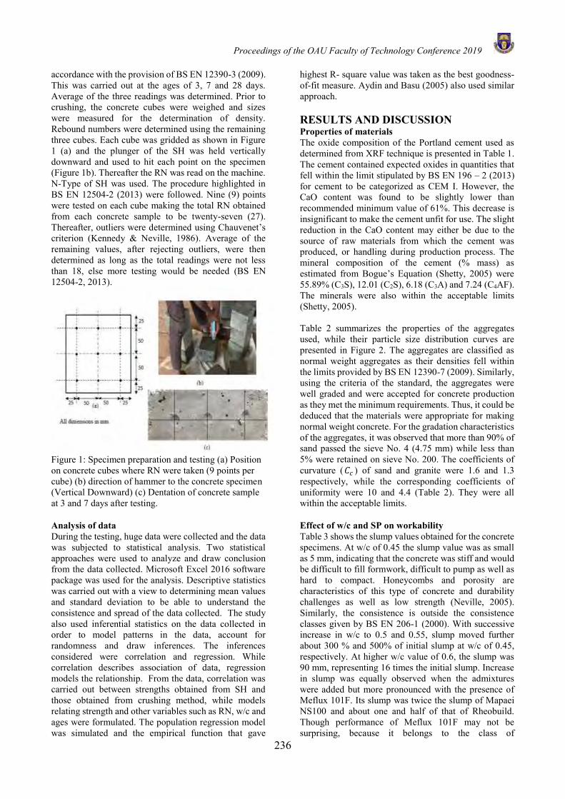
Proceedings of the OAU Faculty of Technology Conference 2019
236
accordance with the provision of BS EN 12390-3 (2009). This was carried out at the ages of 3, 7 and 28 days. Average of the three readings was determined. Prior to crushing, the concrete cubes were weighed and sizes were measured for the determination of density. Rebound numbers were determined using the remaining three cubes. Each cube was gridded as shown in Figure 1 (a) and the plunger of the SH was held vertically downward and used to hit each point on the specimen (Figure 1b). Thereafter the RN was read on the machine. N-Type of SH was used. The procedure highlighted in BS EN 12504-2 (2013) were followed. Nine (9) points were tested on each cube making the total RN obtained from each concrete sample to be twenty-seven (27). Thereafter, outliers were determined using Chauvenet’s criterion (Kennedy & Neville, 1986). Average of the remaining values, after rejecting outliers, were then determined as long as the total readings were not less than 18, else more testing would be needed (BS EN 12504-2, 2013).
Figure 1: Specimen preparation and testing (a) Position on concrete cubes where RN were taken (9 points per cube) (b) direction of hammer to the concrete specimen (Vertical Downward) (c) Dentation of concrete sample at 3 and 7 days after testing.
Analysis of data During the testing, huge data were collected and the data was subjected to statistical analysis. Two statistical approaches were used to analyze and draw conclusion from the data collected. Microsoft Excel 2016 software package was used for the analysis. Descriptive statistics was carried out with a view to determining mean values and standard deviation to be able to understand the consistence and spread of the data collected. The study also used inferential statistics on the data collected in order to model patterns in the data, account for randomness and draw inferences. The inferences considered were correlation and regression. While correlation describes association of data, regression models the relationship. From the data, correlation was carried out between strengths obtained from SH and those obtained from crushing method, while models relating strength and other variables such as RN, w/c and ages were formulated. The population regression model was simulated and the empirical function that gave
highest R- square value was taken as the best goodness-of-fit measure. Aydin and Basu (2005) also used similar approach.
RESULTS AND DISCUSSION Properties of materials The oxide composition of the Portland cement used as determined from XRF technique is presented in Table 1. The cement contained expected oxides in quantities that fell within the limit stipulated by BS EN 196 – 2 (2013) for cement to be categorized as CEM I. However, the CaO content was found to be slightly lower than recommended minimum value of 61%. This decrease is insignificant to make the cement unfit for use. The slight reduction in the CaO content may either be due to the source of raw materials from which the cement was produced, or handling during production process. The mineral composition of the cement (% mass) as estimated from Bogue’s Equation (Shetty, 2005) were 55.89% (C3S), 12.01 (C2S), 6.18 (C3A) and 7.24 (C4AF). The minerals were also within the acceptable limits (Shetty, 2005). Table 2 summarizes the properties of the aggregates used, while their particle size distribution curves are presented in Figure 2. The aggregates are classified as normal weight aggregates as their densities fell within the limits provided by BS EN 12390-7 (2009). Similarly, using the criteria of the standard, the aggregates were well graded and were accepted for concrete production as they met the minimum requirements. Thus, it could be deduced that the materials were appropriate for making normal weight concrete. For the gradation characteristics of the aggregates, it was observed that more than 90% of sand passed the sieve No. 4 (4.75 mm) while less than 5% were retained on sieve No. 200. The coefficients of curvature (𝐶𝑐 ) of sand and granite were 1.6 and 1.3 respectively, while the corresponding coefficients of uniformity were 10 and 4.4 (Table 2). They were all within the acceptable limits.
Effect of w/c and SP on workability Table 3 shows the slump values obtained for the concrete specimens. At w/c of 0.45 the slump value was as small as 5 mm, indicating that the concrete was stiff and would be difficult to fill formwork, difficult to pump as well as hard to compact. Honeycombs and porosity are characteristics of this type of concrete and durability challenges as well as low strength (Neville, 2005). Similarly, the consistence is outside the consistence classes given by BS EN 206-1 (2000). With successive increase in w/c to 0.5 and 0.55, slump moved further about 300 % and 500% of initial slump at w/c of 0.45, respectively. At higher w/c value of 0.6, the slump was 90 mm, representing 16 times the initial slump. Increase in slump was equally observed when the admixtures were added but more pronounced with the presence of Meflux 101F. Its slump was twice the slump of Mapaei NS100 and about one and half of that of Rheobuild. Though performance of Meflux 101F may not be surprising, because it belongs to the class of
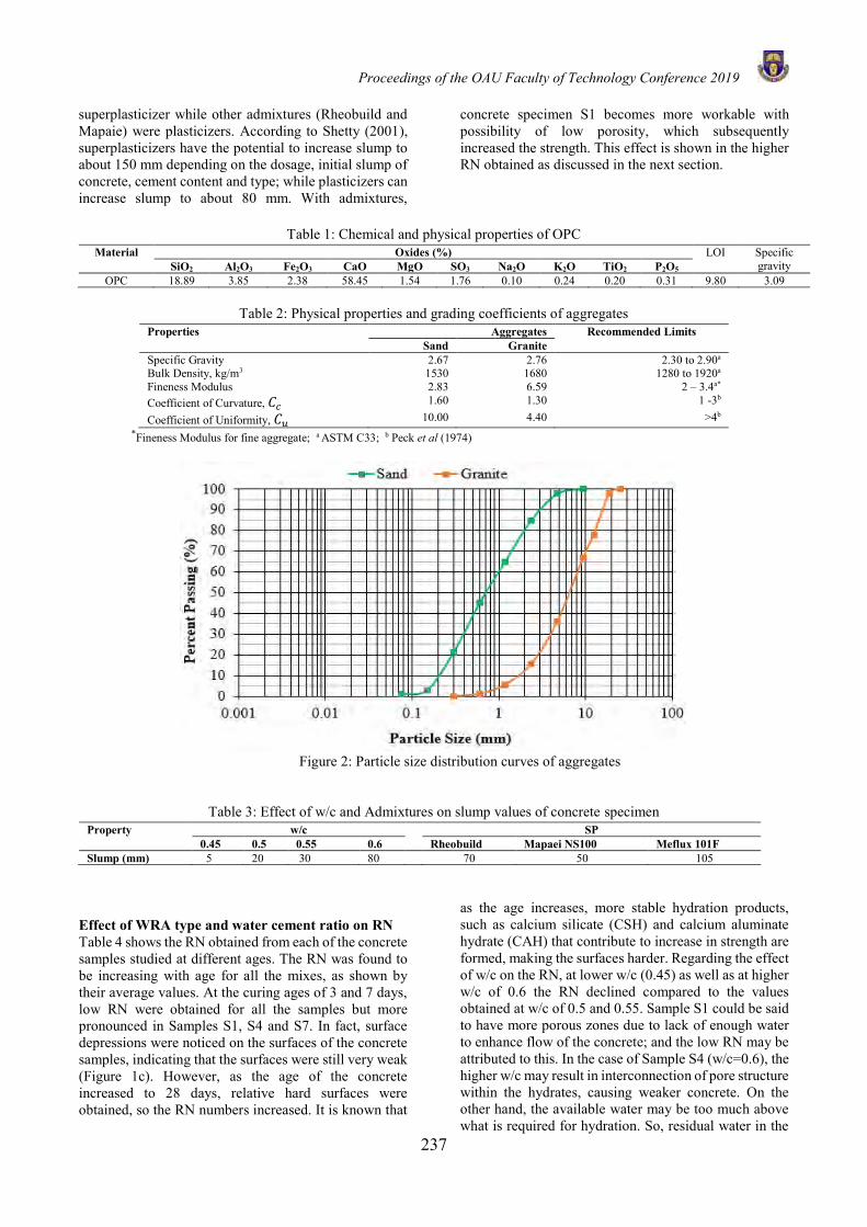
Proceedings of the OAU Faculty of Technology Conference 2019
237
superplasticizer while other admixtures (Rheobuild and Mapaie) were plasticizers. According to Shetty (2001), superplasticizers have the potential to increase slump to about 150 mm depending on the dosage, initial slump of concrete, cement content and type; while plasticizers can increase slump to about 80 mm. With admixtures,
concrete specimen S1 becomes more workable with possibility of low porosity, which subsequently increased the strength. This effect is shown in the higher RN obtained as discussed in the next section.
Table 1: Chemical and physical properties of OPC
Material Oxides (%) LOI Specific gravity SiO2 Al2O3 Fe2O3 CaO MgO SO3 Na2O K2O TiO2 P2O5
OPC 18.89 3.85 2.38 58.45 1.54 1.76 0.10 0.24 0.20 0.31 9.80 3.09
Table 2: Physical properties and grading coefficients of aggregates Properties Aggregates Recommended Limits
Sand Granite Specific Gravity 2.67 2.76 2.30 to 2.90a
Bulk Density, kg/m3 1530 1680 1280 to 1920a
Fineness Modulus 2.83 6.59 2 – 3.4a*
Coefficient of Curvature, 𝐶𝑐 1.60 1.30 1 -3b
Coefficient of Uniformity, 𝐶𝑢 10.00 4.40 >4b
*Fineness Modulus for fine aggregate; a ASTM C33; b Peck et al (1974)
Figure 2: Particle size distribution curves of aggregates
Table 3: Effect of w/c and Admixtures on slump values of concrete specimen Property w/c SP
0.45 0.5 0.55 0.6 Rheobuild Mapaei NS100 Meflux 101F Slump (mm) 5 20 30 80 70 50 105
Effect of WRA type and water cement ratio on RN Table 4 shows the RN obtained from each of the concrete samples studied at different ages. The RN was found to be increasing with age for all the mixes, as shown by their average values. At the curing ages of 3 and 7 days, low RN were obtained for all the samples but more pronounced in Samples S1, S4 and S7. In fact, surface depressions were noticed on the surfaces of the concrete samples, indicating that the surfaces were still very weak (Figure 1c). However, as the age of the concrete increased to 28 days, relative hard surfaces were obtained, so the RN numbers increased. It is known that
as the age increases, more stable hydration products, such as calcium silicate (CSH) and calcium aluminate hydrate (CAH) that contribute to increase in strength are formed, making the surfaces harder. Regarding the effect of w/c on the RN, at lower w/c (0.45) as well as at higher w/c of 0.6 the RN declined compared to the values obtained at w/c of 0.5 and 0.55. Sample S1 could be said to have more porous zones due to lack of enough water to enhance flow of the concrete; and the low RN may be attributed to this. In the case of Sample S4 (w/c=0.6), the higher w/c may result in interconnection of pore structure within the hydrates, causing weaker concrete. On the other hand, the available water may be too much above what is required for hydration. So, residual water in the
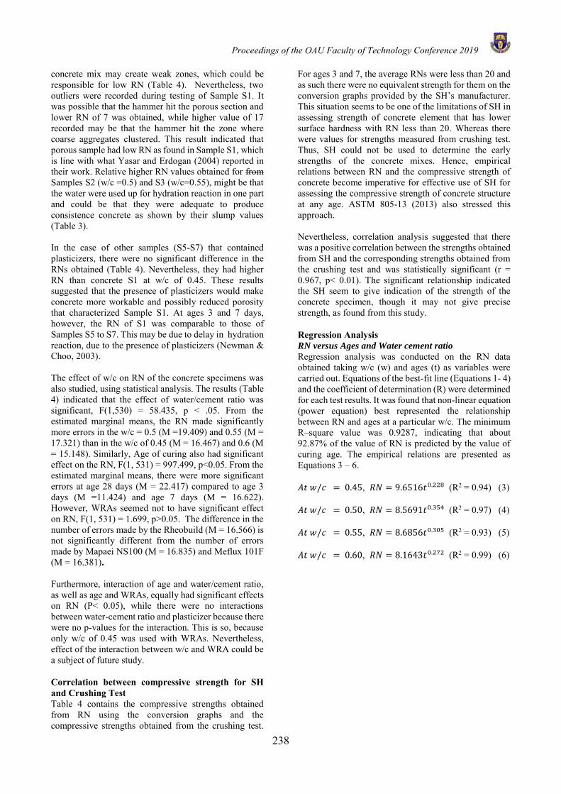
Proceedings of the OAU Faculty of Technology Conference 2019
238
concrete mix may create weak zones, which could be responsible for low RN (Table 4). Nevertheless, two outliers were recorded during testing of Sample S1. It was possible that the hammer hit the porous section and lower RN of 7 was obtained, while higher value of 17 recorded may be that the hammer hit the zone where coarse aggregates clustered. This result indicated that porous sample had low RN as found in Sample S1, which is line with what Yasar and Erdogan (2004) reported in their work. Relative higher RN values obtained for from Samples S2 (w/c =0.5) and S3 (w/c=0.55), might be that the water were used up for hydration reaction in one part and could be that they were adequate to produce consistence concrete as shown by their slump values (Table 3). In the case of other samples (S5-S7) that contained plasticizers, there were no significant difference in the RNs obtained (Table 4). Nevertheless, they had higher RN than concrete S1 at w/c of 0.45. These results suggested that the presence of plasticizers would make concrete more workable and possibly reduced porosity that characterized Sample S1. At ages 3 and 7 days, however, the RN of S1 was comparable to those of Samples S5 to S7. This may be due to delay in hydration reaction, due to the presence of plasticizers (Newman & Choo, 2003). The effect of w/c on RN of the concrete specimens was also studied, using statistical analysis. The results (Table 4) indicated that the effect of water/cement ratio was significant, F(1,530) = 58.435, p < .05. From the estimated marginal means, the RN made significantly more errors in the w/c = 0.5 (M =19.409) and 0.55 (M = 17.321) than in the w/c of 0.45 (M = 16.467) and 0.6 (M = 15.148). Similarly, Age of curing also had significant effect on the RN, F(1, 531) = 997.499, p<0.05. From the estimated marginal means, there were more significant errors at age 28 days (M = 22.417) compared to age 3 days (M =11.424) and age 7 days (M = 16.622). However, WRAs seemed not to have significant effect on RN, F(1, 531) = 1.699, p>0.05. The difference in the number of errors made by the Rheobuild (M = 16.566) is not significantly different from the number of errors made by Mapaei NS100 (M = 16.835) and Meflux 101F (M = 16.381). Furthermore, interaction of age and water/cement ratio, as well as age and WRAs, equally had significant effects on RN (P< 0.05), while there were no interactions between water-cement ratio and plasticizer because there were no p-values for the interaction. This is so, because only w/c of 0.45 was used with WRAs. Nevertheless, effect of the interaction between w/c and WRA could be a subject of future study.
Correlation between compressive strength for SH and Crushing Test Table 4 contains the compressive strengths obtained from RN using the conversion graphs and the compressive strengths obtained from the crushing test.
For ages 3 and 7, the average RNs were less than 20 and as such there were no equivalent strength for them on the conversion graphs provided by the SH’s manufacturer. This situation seems to be one of the limitations of SH in assessing strength of concrete element that has lower surface hardness with RN less than 20. Whereas there were values for strengths measured from crushing test. Thus, SH could not be used to determine the early strengths of the concrete mixes. Hence, empirical relations between RN and the compressive strength of concrete become imperative for effective use of SH for assessing the compressive strength of concrete structure at any age. ASTM 805-13 (2013) also stressed this approach. Nevertheless, correlation analysis suggested that there was a positive correlation between the strengths obtained from SH and the corresponding strengths obtained from the crushing test and was statistically significant (r = 0.967, p< 0.01). The significant relationship indicated the SH seem to give indication of the strength of the concrete specimen, though it may not give precise strength, as found from this study.
Regression Analysis RN versus Ages and Water cement ratio
Regression analysis was conducted on the RN data obtained taking w/c (w) and ages (t) as variables were carried out. Equations of the best-fit line (Equations 1- 4) and the coefficient of determination (R) were determined for each test results. It was found that non-linear equation (power equation) best represented the relationship between RN and ages at a particular w/c. The minimum R–square value was 0.9287, indicating that about 92.87% of the value of RN is predicted by the value of curing age. The empirical relations are presented as Equations 3 – 6.
𝐴𝑡 𝑤/𝑐 = 0.45, 𝑅𝑁 = 9.6516𝑡0.228 (R2 = 0.94) (3)
𝐴𝑡 𝑤/𝑐 = 0.50, 𝑅𝑁 = 8.5691𝑡0.354 (R2 = 0.97) (4)
𝐴𝑡 𝑤/𝑐 = 0.55, 𝑅𝑁 = 8.6856𝑡0.305 (R2 = 0.93) (5)
𝐴𝑡 𝑤/𝑐 = 0.60, 𝑅𝑁 = 8.1643𝑡0.272 (R2 = 0.99) (6)
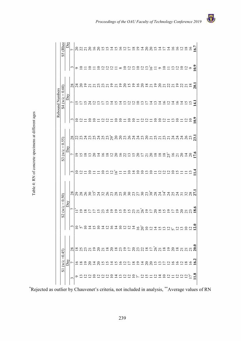
Proceedings of the OAU Faculty of Technology Conference 2019
239
*Rejected as outlier by Chauvenet’s criteria, not included in analysis, **Average values of RN
S/N
Reb
ound
Num
bers
S1 (w
/c =
0.45
)
S2 (w
/c =
0.5
0)
S3
(w/c
= 0
.55)
S4
(w/c
= 0
.60)
S5
(Rhe
obui
ld)
S6
(Map
aei N
S100
) S7
(Mef
lux
101F
)
Day
D
ay
Day
Day
Day
D
ay
D
ay
3
7 28
3
7 28
3
7 28
3
7 28
3
7 28
3
7
28
3 7
28
1 9
16
18
10
11*
29
10
19
22
10
15
24
9 20
22
10
21
22
12
22
20
2
13
18
25
5*
19
28
12
15
23
12
17
20
10
22
21
11
22
22
9 19
23
3
12
19
23
10
18
26
11
18
24
11
15
19
11
21
23
11
19
22
11
17
21
4 12
20
21
1
4 17
30
10
13
23
10
24
21
10
20
20
10
20
22
10
20
22
5
10
14
19
15
17
15*
11
20
25
10
12
21
11
16
20
11
14
22
11
14
24
6 12
20
20
1
0 15
24
11
14
24
11
13
23
10
20
24
12
19
20
12
20
26
7
12
15
21
14
23
32
10
16
25
12
17
23
12
15
25
10
15
20
10
15
23
8 12
15
18
1
2 16
26
13
18
23
12
13
21
12
15
26
13
14
22
9
16
22
9 10
14
20
1
6 19
23
12
12
29
* 11
14
19
12
14
22
12
13
24
12
14
22
10
14
15
18
1
4 19
28
16
* 20
20
10
15
21
11
15
20
12
16
26
12
15
21
11
13
16
23
1
0 15
25
11
16
20
10
14
19
8
16
26
11
16
24
11
16
21
12
12
12
19
12
19
30
11
22
23
11
13
20
10
12
20
11
14
22
11
12
20
13
12
17
17
12
15
30
10
13
26
10
12
15
12
17
23
10
17
23
10
17
20
14
10
18
20
14
23
23
14
15
24
10
12
19
13
18
25
14
18
20
11
18
28*
15
7* 19
23
16
21
27
10
20
24
11
10
16
10
19
21
10
19
20
10
19
20
16
12
14
22
20
* 26
* 30
10
17
23
12
13
20
12
14
20
10
15
23
10
15
22
17
15
20
18
10
19
23
13
21
20
12
17
18
13
20
22
13
19
30
* 13
20
20
18
11
20
17
12
17
38
* 10
20
21
11
14
21
16
* 20
23
10
20
24
10
20
20
19
12
15
26
* 14
20
28
11
18
25
10
13
19
11
15
22
11
15
23
11
15
22
20
14
13
21
15
18
24
12
18
21
10
14
20
9
14
21
12
13
24
12
14
20
21
10
17
18
13
15
14*
12
18
23
12
16
21
10
17
20
14
17
22
10
17
21
22
12
12
19
12
19
24
12
25*
21
11
12
22
11
14
22
12
16
22
12
12
20
23
11
16
20
5* 17
25
10
16
24
13
14
21
13
16
21
10
14
23
10
15
23
24
12
16
18
12
19
24
15
21
24
10
16
19
12
16
23
10
16
22
9
16
24
25
12
12
21
13
20
31
11
20
24
11
14
22
10
12
20
11
12
26
11
12
22
26
12
18
21
10
21
32
11
14
26
12
15
21
12
18
20
11
18
24
11
16
24
27
17*
16
21
12
23
28
13
20
23
10
15
18
9 16
24
13
16
24
13
17
26
A
v.**
11
.8
16.2
20
.0
12.0
18
.6
27.1
11
.4
17.6
23
.1
10.9
14
.1
20.1
10
.9
16.7
22
.1
11.3
16
.6
22.6
10
.9
16.4
21
.9
Tabl
e 4:
RN
of c
oncr
ete
spec
imen
s at d
iffer
ent a
ges

Proceedings of the OAU Faculty of Technology Conference 2019
240
Table 5: RN and compressive strength of the concrete specimens at different curing ages Concrete Specimen
Average RN Strength from SH (N/mm2)
Strength from Crushing (N/mm2)
Curing Ages (Days) Curing Ages (Days) Curing Ages (Days) 3 7 28 3* 7* 28 3 7 28
S1 (c/w =0.45) 11.88 16.18 20.04 - - 15.20 7.31 14.13 19.32 S2 (c/w = 0.50) 12.00 18.56 27.08 - - 25.50 10.23 17.39 27.85 S3 (c/w = 0.55) 11.34 17.58 23.11 - - 19.50 8.68 15.18 23.58 S4 (c/w = 0.60) 10.92 14.04 20.11 - - 15.50 7.13 15.26 21.47 S5 (Rheobuild) 10.88 16.74 22.07 - - 18.00 7.19 14.71 22.35 S6 (Mapaei NS100) 11.30 16.60 22.62 - - 18.50 9.97 13.23 22.12 S7 (Meflux 101F) 10.88 16.41 21.88 - - 16.73 8.74 12.67 20.32
* There is no provision for strength at RN < 20
Interestingly, the difference in the coefficients of the age (t) for all the w/c considered were not significantly different, suggesting that age of the concrete was a major factor influencing the value of RN. Nevertheless, to develop a full picture of effect of age and more exact empirical equations, there is need to consider more ages especially between 7 days and 28 days and/or beyond. Similar trend was observed, when RN was regressed with w/c (w) at ages of 3, 7 and 28 days and the empirical relationships are represented as Equations 7-9. There were strong coefficients of determination between the RN and w/c (w) for all the equations, suggesting that the equations could be used to predict RN once w/c is known for a particular age.
At 3 days, 𝑅𝑁 = −60𝑤2 + 56.2𝑤 – 1.25 (𝑅2 = 0.9304) (7)
𝐴𝑡 7 𝑑𝑎𝑦𝑠: 𝑅𝑁 = −592𝑤2 + 606.8𝑤 −136.96 (𝑅² = 0.9972) (8)
𝐴𝑡 28 𝑑𝑎𝑦𝑠: 𝑅𝑁 = 15973𝑤3 – 26162𝑤2 + 14173𝑤 − 2515.5 ( 𝑅² = 1.000) (9)
Since both w/c and age have been established to have significant impact on the value RN, regression analysis was equally conducted on the data with RN as dependent variable, while w and t were independent variable. The results showed that there was positive and strong correlation between RN and the variables (t and w) (R =0.911). Hence, both t and w have significant effect on
the values of RN (p <0.005). Furthermore, equation of the line of best-fit (Equation 10), has strong coefficient of determination (R2 = 0.8301), indicating that 83% of the variation of the mean value of RN is determined by the combined interaction of age of the concrete (t) and water-cement ratio (w). Therefore, it could be safely concluded that the equation has predictive potential for RN. 𝑅𝑁 = 8𝑡0.3 − 9.707𝑤 + 6.243 (𝑅2 = 0.8302) (10) RN versus compressive strength The main objective of carrying out SH test on concrete is to be able to determine the compressive strength of concrete. Though SH gives RN, which can be related to the hardness of the surface of concrete and further extended to compressive strength. This is achieved by establishing relationship between RN and strength (fc) (Figure 3). The results of regression analysis conducted on the RN data and fc obtained from the crushing tests indicated that coefficient of correlation was 0.96, suggesting that there was a strong and positive relationship. Moreover, empirical function between them is shown in Equation 11, having coefficient of determination of about 0.93. It is possible, therefore, to use this equation to determine compressive strength of the concrete at any age and water-cement ratio within the limit considered in this study. As for other ages or w/c, the equation may be used to give rough estimate of the strength, where preliminary study is required.
Figure 3: RN versus compressive strength
Proceedings of the OAU Faculty of Technology Conference 2019
241
𝑓𝑐 = 0.0095(𝑅𝑁)3 – 0.5909(𝑅𝑁)2 + 12.72(𝑅𝑁) − 72.855 ( 𝑅² = 0.9299) (11)
CONCLUSION Schmidt hammer test was conducted on different concrete specimens made from different water-cement ratio at ages 3, 7 and 28 days. Regression analyses were conducted on the data obtained and the following conclusions were made from the study: i. Water cement ratio and age had significant effect
on the RN of concrete, but admixture dosage did not have influence on the RN.
ii. About 90% of the values of RN are influenced by the values of w/c and age of the concrete.
iii. Conversion tables provided by the manufacture could not account for compressive strength of early age concrete that has RN less than 20.
iv. Regression equation to predict compressive strength of the concrete specimen from the RN were established and had about 92% predictive potential. Thus, the equation could be used to estimate compressive strength of concrete that has RN less than 20.
v. There is need for further study to account for concrete at older ages and effect of direction of application of the
SH on compressive strength.
REFERENCES Amasaki, S. (1991). Estimation of strength of concrete
structures by the rebound hammer. CAJ Proc. Cem. Conc, 45, 345–351.
ASTM C805-13. (2013). Standard Test Method for Rebound Number of Hardened Concrete. American Society for Testing and Materials, West Conshohocken, PA.
Aydin, A., & Basu, A. (2005). The Schmidt hammer in rock material characterization. Eng. Geol, 81, 1–14.
Brozovsky, J. (2012). Implementation of non-destructive impact hammer testing methods in determination of brick strength. Applied Mechanics and Materials, 174–177, 280–285.
BS EN 196 – 2. (2013). Methods of testing cement. Chemical analysis of cement. British Standards Institution.
BS EN 206-1. (2000). Concrete. Specification, performance, production and conformity. British Standards Institution.
BS EN 1097-3. (1998). Tests For Mechanical And Physical Properties Of Aggregates. British Standards Institution.
BS EN 12350-2. (2009). Testing fresh concrete. Slump-test. British Standards Institution.
BS EN 12390-3. (2009). Testing hardened concrete: Compressive strength of test specimens. British Standards Institution.
BS EN 12390-7. (2009). Testing hardened concrete. Density of hardened concrete. British Standards Institution.
BS EN 12504-2. (2013). Testing concrete in structures: non-destructive testing and determination of rebound number. British Standards Institution.
Cargill, J. S., & Shakoor, A. (1990). Evaluation of empirical methods for measuring the uniaxial compressive strength of rock. Int J Rock Mech Min Sci Geomech Abstr, 27, 495–503.
Frauenfelder, R., Laustela, M., & Kääb, A. (2005). Relative age dating of Alpine rock glacier surfaces. Zeitschrift Für Geomorphologie, 49, 145–166.
Grieb, W. (1958). Use of the Swiss Hammer for Estimating the Compressive Strength of Hardened Concrete. FHWA Public Roads,.
IS 13311 (Part 2). (2004). Non-Destructive Testing of Concrete - Methods of Test. Bureau of Indian Standards, new Delhi.
Kennedy, J. B., & Neville, A. M. (1986). Basic Statistical Methods for Engineers and Scientists. Donnelley Publishers.
Kolek, J. (1958). An Appreciation of the Schmidt Rebound Hammer. Magazine of Concrete Research, 10(28), 27–36.
Malhotra, V. M., & Carino, N. J. (2004). Handbook on Nondestructive Testing of Concrete. CRC Press.
Mitchell, L. J., & Hoagland, G. G. (1961). Investigation of the Impact Tube Concrete Test Hammer. Highway Research Board.
Newman, J., & Choo, B. S. (2003). Advanced Concrete Technology - Concrete Properties. Butterworth-Heinemann, Elsevier Ltd., England.
Peck, R. B., Hanson, W. E., & Thornburn, T. H. (1974). Foundation engineering (2nd ed.). John Wiley, New York.
Rubene, S., & Vilnitis, M. (2014). Use of the Schmidt Rebound Hammer for Non Destructive Concrete Structure Testing in Field. Technical Transactions: Civil Engineering, 1-B, 13-19.
Sanchez, K., & Tarranza, N. (2014). Reliability of Rebound Hammer Test in Concrete Compressive

Proceedings of the OAU Faculty of Technology Conference 2019
242
Strength Estimation. International Journal of Advances in Agricultural & Environmental Engg. (IJAAEE), 1(2), 198–202.
Shariati, M., Ramli-Sulong, N. H., Arabnejad, M. M., Shafigh, K. H. P., & Sinaei, H. (2011). Assessing the strength of reinforced concrete structures through Ultrasonic Pulse Velocity and Schmidt Rebound Hammer tests. Scientific Research and Essays, 6(1), 213–220.
Shetty, M. S. (2005). Concrete Technology: Theory and Practice (Multicolour Revised Ed). S. Chand & Company Ltd.New Delhi.
Tamil, S. P., Lakshmi, N. P., & Ramya, G. (2014). Experimental study on concrete using copper slag as replacement material of fie aggregate. Journal of Civil & Environmental Engineering, 4(5), 1–6.
Woodson, R. D. (2009). Evaluating concrete in concrete structures. Concrete Structures, 6, 3–18. https://doi.org/doi:10.1016/b978-1-85617-549-4.00002-2
Yasar, E., & Erdogan, Y. (2004). Estimation of rock physico-mechanical properties using hardness methods. Eng. Geol, 71, 281–288.
Zaky, S. (2001). Evaluation of concrete structural members contained different types of coarse aggregate using Schmidt hammer apparatus after 28-day and at later ages. INTER BUILD, 201–214.
Proceedings of the OAU Faculty of Technology Conference 2019
243
MECHANISM AND MODELS FOR CHLORIDE REMOVAL FROM WASTEWATERS
I.A. OKE1, T. A. ALADESANMI2, S. LUKMAN3, J. S. AMOKO4, O. ADEKUNMBI4, S. O. OJO5, H.O. OLOYEDE4 , M – D. IDI6 and O.T. OYEWOLE2
1Department of Civil Engineering, Obafemi Awolowo University, Ile – Ife, Nigeria 2Information Technology and Communications Unit, Obafemi Awolowo University, Ile- Ife, Nigeria
3 Civil Engineering Department, University of Hafr Al-Batin, Hafr Al-Batin, Saudi Arabia 4Department of Chemistry, Adeyemi College of Education, Ondo; Obafemi Awolowo University, Nigeria.
5 Computer Science and Engineering Department, Obafemi Awolowo University, Ile – Ife, Nigeria 6Land, Air and Water Consulting, Maiduguri, Borno State, Nigeria
E-mail Addresses: [email protected];
ABSTRACT
This paper is a follow-up on our previous studies, which were published as journal articles and contribution to books. The paper provides information on utilization of Microsoft Excel Solver (MES) in the development of models for prediction of chloride removal from selected wastewaters. Carbon resin electrodes were developed from used dry cells and resin using non- heat treatment technique. Performance of the electrodes as anodes during electrochemical treatment process in removing chloride from wastewaters was studied. Effects of selected factors (pH, distance between the electrodes, contact surface area, flow rate, current through the wastewater, treatment time and initial concentration of the chloride) on the performance of the process were evaluated. Models that relate performance of the process to selected factors were developed using MES and statistical methods. The developed models were evaluated statistically(Akaike Information Criterion, (AIC), Schwartz Criterion (SC), coefficient of Determination (CD) and Model of Selection Criterion (MSC)) using expected performance as reference data. The study revealed that at constant current and variable pH, treatment time (F4, 24 = 18.97, p = 3.75 x 10-07) and concentration of chloride (F6, 24 = 12.02, p = 3.16 x 10-06) were significant factors at 99 % confidence level. The models that predict performance of the process based on constant and variable currents were
(%) 3.186 0.080 1.505 0.0006 4.852 9.674 0.0006d a o c t cY X A V A T I= − + − + + + and (%) 93.94 0.116 1.993 0.001 16.284 9.674 0.0087d a o c t cY X A V A T I= − − + − + + − (%) 2752.29 0.195 907.94 18032.64 7764.16 103.20 0.0003d a o c t cY X A V A T I= − − + − + − + and (%) 586.45 0.0051 7.597 1578.23 4282.40 0.00597 0.005d a o c t cY X A V A T I= − + − − + + − for MES and statistical methods,
respectively. It was concluded that MES based model predicted the performance of the treatment process better than statistical based model based on the MSC, AIC, CD and SC.
Keywords: Chlorine, Electrochemical treatment, carbon-resin electrodes, Statistical Evaluation, Microsoft Excel Solver
INTRODUCTION Water is an essential element of life for both animals and plants. Potable and safe drinking water require specific treatment processes to remove various contaminants from it. It has been reported that access to safe and potable drinking water has great influence on the health status, economic value and quality of life of the human. Assessment of water quality and availability to people in the various regions of the world by World Health Organization (WHO) revealed that at least 5 million deaths per year are recorded due to the utilization of unsafe drinking water and not less than 1.4 billion are without access to potable and safe drinking water (Fehintola et al., 2015). It has been reported that most of these deaths took place in developing countries of the world which include Ghana, Nigeria, Somalia, Kenya, India etc. Ishaku et al. (2011) and Fehintola et al. (2015) reported that more than 1.2 billion people did not have access to improved water source, which indicates that these people have to revert to unprotected wells, polluted springs, open canals, contaminated lakes and rivers to
fetch water for use in the house. Provision of safe and potable water is one of the major challenges facing the rural communities of Nigeria today. It has been reported that over 70 % of households in rural communities in Nigeria do not have access to improved water supply. These rural communities depend mainly on self-water supply (free water sources, such as rivers, perennial streams, water ponds and unprotected wells) which is vulnerable to water borne diseases (typhoid fever, cholera, dysentery etc. Ishaku et al., 2011; Fehintola et al., 2015). Recent snapshot of drinking water and sanitation in Africa 2017 update shows that Nigeria is not on track towards the Millennium Development Goals (MDGs) in respect to drinking water and sanitation practises target ( JMP, 2018). More on access to safe water in Nigeria can be found in literature such as Otun et al. (2011); Ince et al. (2013). Literature reported that larger volume of water in the planet is in the form of sea water. Sea water is known to be contaminated with high concentration of chloride ion, which must be removed or reduced to the lowest level (250 mg/l). Electrochemical,
Proceedings of the OAU Faculty of Technology Conference 2019
244
distillation and membrane methods are the important methods for salty water purification. It has been reported that the last two methods are more expensive and require high technologies when in operation than former process. It is therefore necessary to evaluate alternative methods for chloride removal from salty water such as sea water using electrochemical process. More on electrochemical treatment process of water and wastewaters can be found in literature such as Chen (2004), Khemis et al. (2006), Diaz et al. (2008), Oke (2009). The main focus of this study is to evaluate the performance of electrochemical treatment process with carbon –resin electrodes for chloride removal from aqueous salty water. MATERIALS AND METHODS Carbon resin electrodes were developed from used dry cell and resin using non-heat treatment technique. Synthetic wastewaters containing known concentrations of chloride (as individual and combination with other ions, between 500 and 15000 mg/l, Oke, 2009) were prepared and subjected to electrochemical treatment process using carbon – resin electrodes. Chloride determination in both treated and untreated wastewaters were carried out using procedures specified in Standard
Methods for Water and Wastewater Examination (APHA, 2012, van Loosdrecht et al., 2016). Chloride concentrations removed (R, %) during the treatment process were computed as follows:
−=
0
0100(%)C
CCR t (1)
Where, Co and Ct are the initial and final concentrations of chloride, respectively (mg/l). Performance of the electrodes as anodes during electrochemical treatment process in removing chloride from wastewaters was studied. Effects of selected factors (pH, distance between the electrodes, contact surface area, flow rate, current through the wastewater, treatment time, co-ions concentrations and initial concentration of the chloride) on the performance of the process were evaluated. Model that relates the performance of the process to selected factors were developed using MES and statistical methods. The models were evaluated statistically (Akaike Information Criterion, (AIC), Schwartz Criterion (SC), coefficient of Determination (CD) and Model of Selection Criterion (MSC)) using expected value as reference data). The statistical model equations are as shown in Equations 2-8.
1 1 1
1 1 1 1(2)
n n n
d ai i it
n n n n
o c ci i i it
R nA B X C A
D V E A F T G I
= = =
= = = =
= + + +
+ + +
1 1 1 1
1 1 1 1(3)
n n n n
d d d d d ai i i it
n n n n
d o d c d d ci i i it
X R A X B X X C X A
D X V E X A F X T G X I
= = = =
= = = =
= + + +
+ + +
1 1 1 1
1 1 1 1(4)
n n n n
a a a d a ai i i it
n n n n
a o a c a a ci i i it
A R A A B A X C A A
D A V E A A F A T G A I
= = = =
= = = =
= + +
+ + + +
1 1 1 1
1 1 1 1(5)
n n n n
o o o d o ai i i it
n n n n
o o o c o o ci i i it
V R A V B V X C V A
D V V E V A F V T G V I
= = = =
= = = =
= + +
+ + + +
1 1 1 1
1 1 1 1(6)
n n n n
c t c c d c ai i i i
n n n n
c o c c c t c ci i i i
A R A A B A X C A A
D A V E A A F A T G A I
= = = =
= = = =
= + +
+ + + +
1 1 1 1
1 1 1 1(7)
n n n n
t t t t d t ai i i i
n n n n
t o t c t t t ci i i i
T R A T B T X C T A
D TV E T A F TT G T I
= = = =
= = = =
= + +
+ + + +
1 1 1 1
1 1 1 1(8)
n n n n
c t c c d c ai i i i
n n n n
c o c c c t c ci i i i
I R A I B I X C I A
D I V E I A F I T G I I
= = = =
= = = =
= + +
+ + + +
Where; Rt, Ac, Xd, Aa,Vo, Ti, Ic and n are chloride removed, surface area of electrode, separation distance
between electrodes, current through the wastewater, volume of the wastewater, treatment time, initial concentration of chloride and number of samples, respectively. A, B, C, D, E , F and G are model’s constants. Procedures employed in the computations of model constants using Microsoft Excel Solver (MES) are as follows (Oke et al., 2017):
a) Microsoft Excel Solver was added in on the toolbar of Microsoft Excel;
b) Target (limit) value of the iteration was set for the software based on square of difference as
( ) 2
10
n
t d a o c t ci
R A BX CA DV EA FT GI=
− + + + + + + = ; (9)
c) Changing cells of the iterations were selected, number of iterations, degree of accuracy and maximum time for the iteration were set for the software to meet the target; and
d) The iteration started through Microsoft Excel Solver (Figure 1).
More on MES can be found in literature such as Oke et al. (2016; 2017), Barati (2013); Tay et al. (2014) and Hui et al. (2018). Figures 2 and 3 present laboratory setup of the electrochemical treatment process. The Model of Selection Criterion (MSC) is interpreted as the proportion of expected chloride concentration and observed chloride concentrations variation that can be explained by the obtained chloride concentrations. Higher value of MSC indicates higher accuracy, validity and the good fitness of the method. MSC was computed using equation (10) as follows:
Proceedings of the OAU Faculty of Technology Conference 2019
245
( )
( )np
YY
YYMSC
n
icaliobsi
n
iobsobsi
2ln 2
1
2
1 −
−
−
=
=
= (10) where
Yobsi is the observed concentration; obsY is the average of observed concentration; p is the total number of fixed parameters to be estimated in the equation; n is the total number of concentration, and Ycali is the expected concentration. The AIC was derived from the Information Criterion of Akaike (1976). It allows a direct comparison among models with a different number of parameters. The AIC presents the information on a given set of parameter estimates by relating the coefficient of determination to the number of parameters. The AIC values were computed using Equation (11).
( ) pYYnAICn
icaliobsi 2ln
2
1
+
−= =
(11)
The Schwartz Criterion (SC) is defined by Equation (12).
( )2
1ln ln( )
n
obsi calii
SC n Y Y p n=
= − +
(12)
The more appropriate model is the one with the smaller SC value. Coefficient of determination (CD) can be interpreted as the proportion of expected data variation that can be explained by the obtained data. Higher values of CD indicate higher accuracy, validity and good fitness of the method. CD can be expressed as Equation (13).
( ) ( )
( )2
1
2
1
2
1
=
==
−
−−−=
n
icaliobsi
n
icaliobsi
n
icaliobsi
YY
YYYYCD (13)
RESULTS AND DISCUSSION The results of the treatment options are as presented in Figures 4, 5, 6 and 7. Figures 8 to 11 present more information on chloride removal. These figures revealed that removal of chloride ion by electrochemical treatment with carbon – resin system ranges from 20 to 95.4 %. Lower efficacy of the system during controlled system can be attributed to Joule heating energy loss and energy used by the rheostat used in regulating the current. This indicates that part of the energy supplied was used as heat energy by both the electrodes and rheostat. Similarly, lower efficacy in chloride ion removal can be attributed to the following factors:
i. the presence of co-ions which also used part of the energy and
ii. competitive adsorption by the ions present For combination systems lower reduction in chloride ion removal can be attributed to the two factors mentioned
above and the presence of cations such as chromium and cadmium. It has been postulated that in the presence of carbon (activated carbon) chromium (VI) may be reduced to chromium (III) as follows:
2 34 2 23 4 2 4 3 10C CrO OH Cr CO H O− − ++ + → + + (14)
Equation (14) revealed that spent carbon particles (from carbon – resin) were converted to carbon (IV) oxide in the presence of chromium in system, which indicates that reduction in chloride ion by adsorption was made impossible. The figures show that efficacy of the system increases with increasing initial concentration of chloride ion, treatment time and current through the electrolyte. This indicates that chloride ion removal by electrochemical method is a function of current, time and initial concentration. It was noticed that efficacy of the treatment process decreased with decrease in concentration of the pollutant and with treatment time (more energy was required to remove the same amount of chloride when initial concentration is lower than when initial concentration is higher). It was observed generally that chloride removal at the anode was in two stages (through electrolysis, adsorption and or reactions). In the first stage it was experienced that high concentrations of chlorine gas were evolved at the anode indicating that chloride ions were oxidized to chlorine gas (Equation 15) but the intensity decreases with treatment period(Oke et al., 2016).
22 nClennCl oxidation⎯⎯⎯ →⎯−− (15)
In the second stage, chlorine gas was not evolved but reduction in chloride ions was observed. These phenomena in the second stage may be attributed to adsorption of chloride ions by spent carbon particles (carbon as an adsorbent and chloride ion as an adsorbate) or may be attributed to reaction between chlorine gas in water as presented in Equation (16) in which residual chlorine is the end product rather than chlorine gas, but it was observed that the higher the particles the higher chloride ion removal. This result confirms Feleke et al. (1998) conclusions on chloride removal from wastewaters electrochemically that chloride can be removed by electrochemical treatment to a level that will not harm micro -organisms during biological treatment. Further studies on effects of pH, current and treatment time (energy) used on efficacy of the method revealed that energy used (Current and time) could significantly influence efficacy of electrochemical treatment method. This may be attributed to two main reactions, namely:
i. electro- oxidation ; and ii. physical and chemical adsorption of chloride
ions.
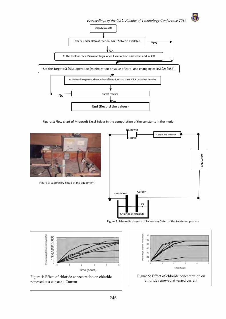
Proceedings of the OAU Faculty of Technology Conference 2019
246
Open Microsoft
Excel
Check under Data at the tool bar if Solver is available
No
Yes
At the toolbar click Microsoft logo, open Excel option and select add in. OK
Set the Target ($L$53), operation (minimization or value of zero) and changing cell($k$2: $k$6)
At Solver dialogue set the number of iterations and time. Click on Solver to solve
Target reached
End (Record the values)
Yes
No
Figure 1: Flow chart of Microsoft Excel Solver in the computation of the constants in the model
Figure 2: Laboratory Setup of the equipment
Control and Rheostat
Am
meter
DC power
source
Figure 3: Schematic diagram of Laboratory Setup of the treatment process
aluminium Carbon-
resin
Chloride electrolyte
Figure 4: Effect of chloride concentration on chloride removed at a constant. Current
Figure 5: Effect of chloride concentration on chloride removed at varied current
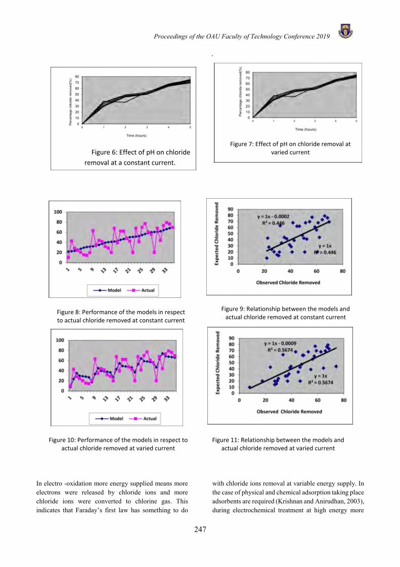
Proceedings of the OAU Faculty of Technology Conference 2019
247
.
In electro -oxidation more energy supplied means more electrons were released by chloride ions and more chloride ions were converted to chlorine gas. This indicates that Faraday’s first law has something to do
with chloride ions removal at variable energy supply. In the case of physical and chemical adsorption taking place adsorbents are required (Krishnan and Anirudhan, 2003), during electrochemical treatment at high energy more
Figure 8: Performance of the models in respect to actual chloride removed at constant current
Figure 9: Relationship between the models and actual chloride removed at constant current
Figure 10: Performance of the models in respect to actual chloride removed at varied current
Figure 11: Relationship between the models and actual chloride removed at varied current
Figure 6: Effect of pH on chloride
removal at a constant current.
Figure 7: Effect of pH on chloride removal at varied current
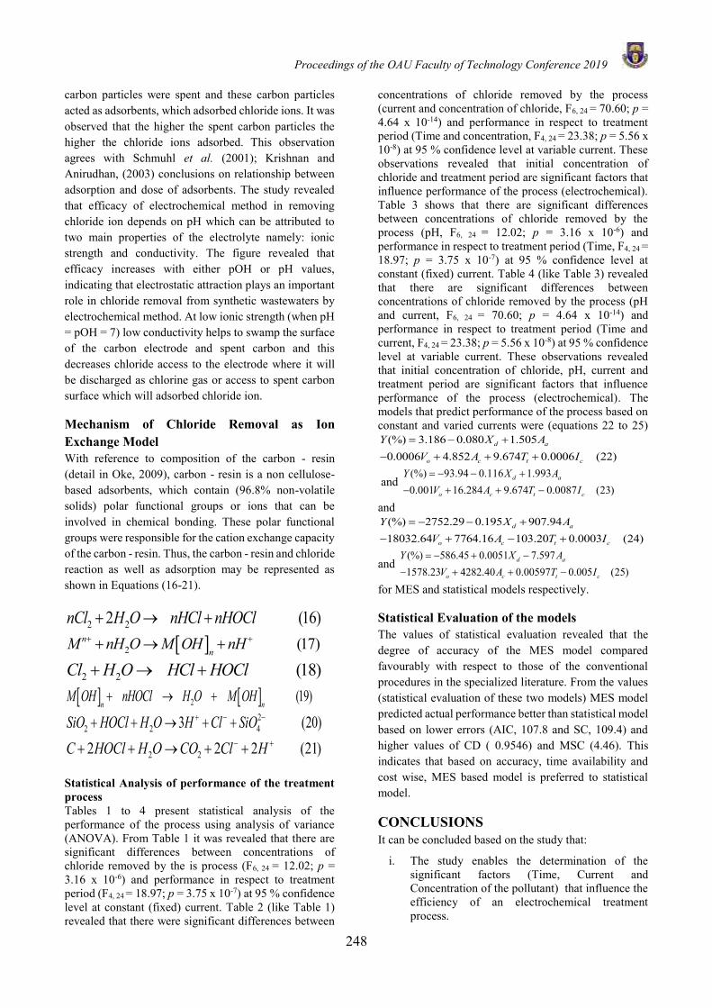
Proceedings of the OAU Faculty of Technology Conference 2019
248
carbon particles were spent and these carbon particles acted as adsorbents, which adsorbed chloride ions. It was observed that the higher the spent carbon particles the higher the chloride ions adsorbed. This observation agrees with Schmuhl et al. (2001); Krishnan and Anirudhan, (2003) conclusions on relationship between adsorption and dose of adsorbents. The study revealed that efficacy of electrochemical method in removing chloride ion depends on pH which can be attributed to two main properties of the electrolyte namely: ionic strength and conductivity. The figure revealed that efficacy increases with either pOH or pH values, indicating that electrostatic attraction plays an important role in chloride removal from synthetic wastewaters by electrochemical method. At low ionic strength (when pH = pOH = 7) low conductivity helps to swamp the surface of the carbon electrode and spent carbon and this decreases chloride access to the electrode where it will be discharged as chlorine gas or access to spent carbon surface which will adsorbed chloride ion.
Mechanism of Chloride Removal as Ion Exchange Model With reference to composition of the carbon - resin (detail in Oke, 2009), carbon - resin is a non cellulose-based adsorbents, which contain (96.8% non-volatile solids) polar functional groups or ions that can be involved in chemical bonding. These polar functional groups were responsible for the cation exchange capacity of the carbon - resin. Thus, the carbon - resin and chloride reaction as well as adsorption may be represented as shown in Equations (16-21).
2 22 (16)nCl H O nHCl nHOCl+ → +
2 (17)nn
M nH O M OH nH+ ++ → +
2 2 (18)Cl H O HCl HOCl+ → +
2 (19)n n
M OH nHOCl H O M OH+ → +2
2 2 43 (20)SiO HOCl H O H Cl SiO+ − −+ + → + +
2 22 2 2 (21)C HOCl H O CO Cl H− ++ + → + + Statistical Analysis of performance of the treatment process Tables 1 to 4 present statistical analysis of the performance of the process using analysis of variance (ANOVA). From Table 1 it was revealed that there are significant differences between concentrations of chloride removed by the is process (F6, 24 = 12.02; p = 3.16 x 10⁻⁶) and performance in respect to treatment period (F4, 24 = 18.97; p = 3.75 x 10⁻⁷) at 95 % confidence level at constant (fixed) current. Table 2 (like Table 1) revealed that there were significant differences between
concentrations of chloride removed by the process (current and concentration of chloride, F6, 24 = 70.60; p = 4.64 x 10⁻¹⁴) and performance in respect to treatment period (Time and concentration, F4, 24 = 23.38; p = 5.56 x 10⁻⁸) at 95 % confidence level at variable current. These observations revealed that initial concentration of chloride and treatment period are significant factors that influence performance of the process (electrochemical). Table 3 shows that there are significant differences between concentrations of chloride removed by the process (pH, F6, 24 = 12.02; p = 3.16 x 10⁻⁶) and performance in respect to treatment period (Time, F4, 24 = 18.97; p = 3.75 x 10⁻⁷) at 95 % confidence level at constant (fixed) current. Table 4 (like Table 3) revealed that there are significant differences between concentrations of chloride removed by the process (pH and current, F6, 24 = 70.60; p = 4.64 x 10⁻¹⁴) and performance in respect to treatment period (Time and current, F4, 24 = 23.38; p = 5.56 x 10⁻⁸) at 95 % confidence level at variable current. These observations revealed that initial concentration of chloride, pH, current and treatment period are significant factors that influence performance of the process (electrochemical). The models that predict performance of the process based on constant and varied currents were (equations 22 to 25)
(%) 3.186 0.080 1.5050.0006 4.852 9.674 0.0006 (22)
d a
o c t c
Y X AV A T I
= − +
− + + +
and (%) 93.94 0.116 1.9930.001 16.284 9.674 0.0087 (23)
d a
o c t c
Y X AV A T I
= − − +
− + + −
and (%) 2752.29 0.195 907.9418032.64 7764.16 103.20 0.0003 (24)
d a
o c t c
Y X AV A T I
= − − +
− + − +
and (%) 586.45 0.0051 7.5971578.23 4282.40 0.00597 0.005 (25)
d a
o c t c
Y X AV A T I
= − + −
− + + −
for MES and statistical models respectively. Statistical Evaluation of the models The values of statistical evaluation revealed that the degree of accuracy of the MES model compared favourably with respect to those of the conventional procedures in the specialized literature. From the values (statistical evaluation of these two models) MES model predicted actual performance better than statistical model based on lower errors (AIC, 107.8 and SC, 109.4) and higher values of CD ( 0.9546) and MSC (4.46). This indicates that based on accuracy, time availability and cost wise, MES based model is preferred to statistical model.
CONCLUSIONS It can be concluded based on the study that:
i. The study enables the determination of the significant factors (Time, Current and Concentration of the pollutant) that influence the efficiency of an electrochemical treatment process.

Proceedings of the OAU Faculty of Technology Conference 2019
249
ii. MES predicted the performance of the treatment process better than statistical model based on the values of MSC, AIC, CD and SC.
ACKNOWLEDGEMENT The authors wish to acknowledge Obafemi Awolowo University, Ile-Ife (Nigeria) for funding the project
through University Research Committee (URC) under the grant number 11- 812- AUW and members of staff of Department of Materials Science and Engineering, Obafemi Awolowo University, Ile-Ife (Nigeria) for providing tools and equipment used in the development of the electrodes. We wish to thank Elizade University, Ilara – Mokin for conference attendance support
.
Table 1: ANOVA of effect of time and initial Chloride Concentration at constant current
Source of Variation Sum of Squares
Degree of freedom Mean Square F-value P-value F crit
Concentration 6514.65 6 1085.775 12.022 3.16 x 10-06 2.508189
Time 6853.333 4 1713.333 18.970 3.75 x 10-07 2.776289
Error 2167.607 24 90.3167 Total 15535.59 34
Table 2: ANOVA of effect of time and initial Chloride Concentration at varied current
Source of Variation Sum of Squares
Degree of freedom
Mean Square F-value P-value F crit
Current and Concentration 21034.75 6 3505.791 70.60191 4.64 x 10⁻¹⁴ 2.508189
Time and concentration 4643.152 4 1160.788 23.37671 5.56 x 10-08 2.776289
Error 1191.738 24 49.65575 Total 26869.64 34
Table 3: ANOVA of effect of time and initial pH at constant current
Source of Variation Sum of Squares
Degree of freedom
Mean Square F-value P-value F crit
pH 73.324 6 12.22067 2.029441 0.1008 2.508189
Time 6695.218 4 1673.805 277.9625 1.01 x 10⁻¹⁹ 2.776289
Error 144.5206 24 6.021692 Total 6913.063 34
Table 4: ANOVA of effect of time and initial pH at varied current
Source of Variation Sum of Squares
Degree of freedom
Mean Square F-value P-value F crit
pH and Current 54.84438 6 9.14073 1.88197 0.11677 2.420523
Time and current 23868.01 5 4773.603 982.8293 2.72 x 10⁻³² 2.533555
Error 145.71 30 4.857001
Total 24068.57 41
REFERENCES Akaike, H. (1976). An information criterion (AIC),
Math. Sci. 14,1-5. APHA, (2012). Standard Method for the
Examination of Water and Wastewater, 22nd edn, America Water Works Association and Water Pollution Control Federation, Washington DC.
Barati, R (2013) Application of Excel Solver for Parameter Estimation of the Nonlinear
Muskingum Models. KSCE Journal of Civil Engineering, 17(5):1139-1148
Chen, G (2004). Electrochemical technologies in wastewater treatment Separation. Purification Technologies 38(1), 11-41
Díaz, B.C, B; Bilyeu, G; Morales,R and Hernández. P. B. (2008). A Comparison of Iron and Aluminium Electrodes in Hydrogen Peroxide-Assisted Electrocoagulation of Organic
Proceedings of the OAU Faculty of Technology Conference 2019
250
Pollutants. Environmental Engineering Science, 25 (4), 529-538.
Feleke, Z; Araki, K; Sakakibara, Y; Watanabe, T and Kuroda, M (1998). Selective reduction of nitrate to nitrogen gas in a biofilm-electrode reactor. Water Research, 32 (9), 2728-2734
Fehintola, E. O , Amoko, J. S, Obijole, O. A. and Oke, I. A.(2015). Pseudo second order kinetics model of adsorption of Pb2+ onto powdered corn cobs: comparison of linear regression methods. Direct Research Journal of Chemistry and Material Science (DRCMS. 3(1), 1 -10
Hui, Z., Xue, Z., Luobin W., Kai, W. and Wendong, W. (2018) Development of a software tool for teaching real‐time state simulation of water distribution networks, Computer Applications in Engineering Education, 26 (3), 577-588.
Ince, M; D. Bashir, O.O.O. Oni, E.O. Awe, V. Ogbechie, K. Korve, M.A. Adeyinka, A.A. Olufolabo and F.Ofordu (2013). Rapid Assessment of Drinking Water Quality (RADWQ) Country Report: Nigeria. WHO and UNICEF
Ishaku, H. T.;, M. Rafee Majid, A. P. Ajayi and , A. Haruna (2011). Water Supply Dilemma in Nigerian Rural Communities: Looking towards the Sky for an Answer. Journal of Water Resource and Protection, 3, 598-606
JMP (2018) update Progress on sanitation and drinking-water - 2017 update (http://www.who.int/about/licensing/copyright_form/en/ accessed on 25th January, 2019
Khemis, M., Leclerc, J.P., Tanguy, G., Valenti˙N, G., and Lapicque, F. (2006). Treatment of industrial liquid wastes by electrocoagulation: Experimental investigations and an overall interpretation model. Chem. Eng. Sci. 61, 3602.
Krishnan, K.A and Anirudhan, T.S (2003). Removal of cadmium II from aqueous solutions by steam activated sulphonised carbon prepared from sugar –cane bagasse pith: kinetic and equilibrium studies . Water SA, 29(2) 147-156.
Oke, I. A (2009) Orthogonal Experiments in the Development of Carbon –Resin For Chloride Ions Removal. Statistical Methodology. 6, 109–119.
Oke, I. A. ; Ismail, A. ; Lukman, S. ; S. O. Ojo, O. O. Adeosun, and M. O. Nwude (2016). Economics and Statistical Evaluations of Using Microsoft Excel Solver in Pipe Network Analysis. J. Pipeline Syst. Eng. 7(4): 06016002-1- 9
Oke, I. A.; Lukman, S. and Ismail, A(2017). Development And Performance Evaluation Of A New Numerical Model For Groundwater Recharge Estimation. Nigeria Journal of Engineering , 23(2), 56 -65.
Otun, J. A. ; I.A. Oke and A.M. Oguntuase.(2011) Issues and Challenges of Decaying Urban Water Infrastructures in Nigeria. 35th WEDC International Conference, Loughborough, UK, July 2011
Schmuhl, R; Kneg, H.M and Keizer, K .(2001)Adsorption of Cu(II) and Cr(VI) ions by chitosan, kinetic and equilibrium studies , Water SA, 27(1), 1-5.
Tay, K. G; Kek, S. L. and Rosmila A. K. (2014). Solving Non-Linear Systems by Newton’s Method Using Spreadsheet Excel.
van Loosdrecht, M.C.M., Nielsen, P.H.,Lopez-Vazquez, C.M., Brdjanovic, D., (2016). Experimental Methods in Wastewater Treatment. 1st Edition, International Water Publishing Alliance House, London.

Proceedings of the OAU Faculty of Technology Conference 2019
251
MODEL IDENTIFICATION OF BIOMASS BOILER SYSTEM USING PRINCIPAL COMPONENT REGRESSION
T. A. Morakinyo*1 and C. T. Akanbi1
1Department of Food Science and Technology Obafemi Awolowo University, Ile-Ife, Nigeria.
*Email of Corresponding Author: [email protected]
ABSTRACT The focus of this study was to identify boiler operational variables that positively and negatively contributed to the boiler biomass utility using Principal Component Regression (PCR) to enhance its thermal efficiency. An installed biomass fired vertical boiler was developed and evaluated by combusting 30.0 kg of charcoal to generate superheated steam within 3.0 hrs. Biomass utility was chosen as independent variable while steam pressure, steam chamber temperature, superheat steam flow rate, exhaust gas temperature, inner and outer insulated wall temperatures were dependent variables. Experimental data obtained were recorded values of dependent variables against independent at an interval of 10 minutes. The factor analysis of Biplot model was adopted to categorise the variables into two; hence factor loading was validated using STATISTICAL 12 factor analysis model. The correlation between variables and factors was established to determine the level of significance and validated using squared cosines and percentage of contribution of each variable. The result showed that the coefficient of determinations of both factors analyses using principal component regression model fit the measured responses at levels of 99.40% and 95.07%, respectively. The principal component regression model indicated that superheated steam flow rate and steam pressure contributed positively while steam chamber temperature, exhaust gas temperature, inner and outer insulated wall temperatures contributed negatively to biomass utility. This indicated that the rest of the system variables apart from the steam pressure and the superheated steam flow rate reduce biomass utility which increases the cost of operation of the newly developed boiler. Conclusively, the variables required further modification had been identified to eradicate heat losses and enhance thermal efficiency.
Keywords: Operational boiler variables, Principal component regression models, Greenhouse gases, Biomass fired boiler, Steam generation.
INTRODUCTION The development and further modifications of indigenous steam generators of various capacities is required in Africa for economic and industrial emancipation. In the United State of America, about 1.3 million of boilers of different types and capacities were installed and monitored at industrial, commercial and institutional settings for further modifications (Panel, 2009). Boiler is the major unit operation in any power generation turbine plant. However, poor thermal efficiency and inefficient energy conservation in boiler design will increase its running cost and generate greenhouse gases that support global warming (Oyedepo, 2012). The generated steam has wider applications that cover about 35-40% of energy usage in industry globally (UNIDO, 2016). These applications are energy conversion systems, food processes and production support in confectionary, brewery, sugar, salt, oilseeds, dairy, paper, petroleum, chemicals, plastics, rubber, textile, pharmaceuticals, and refining and primary metals industries. Furthermore, other areas of steam applications are: heat and mass transfer process (drying, blanching, hermetical sterilization and separation), power generation plants, water treatment, cleaning in place (CIP) of the units operation, packaging (gum melting), storage, waste management, heating of buildings, dry cleaners and laundries (UNIDO, 2016). Hence, the advantages of steam utilization in industry cannot be over emphasized
due to some peculiar characteristics such as: constant temperature, high heat transfer coefficient, highest latent heat per unit mass, and extremely cost effective and high flexible energy transfer factor (Lienhard and Lienhard, 2017). Over decades, different types of steam generator, commonly referred to as boiler had been developed to suit aforementioned purposes. The industrial boiler can be classified into two namely: water-in-tube and fire-in-tube (Master et al., 2003; Yang et al., 2018; Morakinyo and Bamgboye, 2016). Previous researchers reported that biomass has potential for energy generation due to its availability at low price, renewable energy source coupled with carbon neutral features (Ojolo et al., 2012; Orisalaye et al., 2018).
The efficiency of any boiler can be rated on how effective its net input thermal energy can be converted optimally to thermal energy output (Reddy and Reddy, 2013). It has also been reported that the economical operation of any boiler depends on its thermal efficiency rating (Wang et al., 2014). Several factors that contributed to this efficiency are: boiler variables, accessories status, types of fuel and moisture content value, level of scaling and climatic conditions, optimum stoichiometric fuel and air ratio, adequate maintenance of heat transfer surfaces, installation of heat recovery equipment, add or replace boiler refractory effectively, standardizing and regular calibration of fuel (Shah and Adhyaru, 2011; Wang et al.,
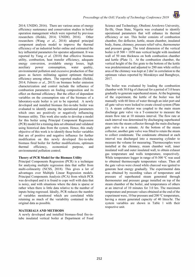
Proceedings of the OAU Faculty of Technology Conference 2019
252
2014; UNIDO, 2016). There are various areas of energy efficiency sustenance and conservation studies in boiler operation management which were reported by previous researchers (Heikki, 2014; UNIDO, 2016). Other researchers (Wang et al., 2014) adopted principal component analysis model to improve the thermal efficiency of an industrial boiler online and estimated the key influential parameters for operator adjustment. It was reported by Yang et al. (2018) that effective biomass utility, combustion, heat transfer efficiency, adequate energy conversion, avoidable energy losses, high auxiliary power consumption, water quality, environmental pollution and excessive production of flue gases as factors militating against optimum thermal efficiency among others. The reported studies (Heikki, 2014; Febrero et al., 2015) on biomass boiler emission characterization and control include the influence of combustion parameters on fouling composition and its effect on thermal efficiency. But the effect of dependent variables on the consumption rate of the biomass of a laboratory-scale boiler is yet to be reported. A newly developed and installed biomass fire-in-tube boiler was evaluated to identify among the operational parameters which ones are positively or negatively influencing biomass utility. This work also seeks to develop a model for this boiler using Principal Component Regression (PCR) model for a training data set obtained and validated using historical data from the system. Hence, this study objective of this work is to identify those boiler variables that are of positive and negative influence for further modification on this newly developed fire-in-tube biomass fired boiler for further modifications, optimum thermal efficiency, economical purpose, and environmental pollution control.
Theory of PCR Model for the Biomass Utility Principal Components Regression (PCR) is a technique for analysing multiple regression data that suffer from multi-colinearity (NCSS, 2018). This gives a lot of advantages over Multiple Linear Regression models. Principal Components Analysis (PCA) from which PCR was developed and it is found to cope well with data that is noisy, and with situations where the data is sparse or rather when there is little data relative to the number of inputs being regressed. Ideally, PCR reduces the number of variables monitored which are correlated while retaining as much of the variability contained in the original data as possible. MATERIALS AND METHODS A newly developed and installed biomass-fired fire-in-tube insulated vertical boiler at Department of Food
Science and Technology, Obafemi Awolowo University, Ile-Ife, Osun State, Nigeria was evaluated to identify operational parameters that will enhance its thermal efficiency or not. This boiler consists of combustion chamber, fire deflector, kettle, steam chamber, insulated body, frame, chimney, pressure relief valve, thermometer and pressure gauge. The total dimension of the vertical boiler is Ø 500 × 1050 mm vertical height with insulated wall of 50 mm thickness on both combustion chamber and kettle (Plate 1). At the combustion chamber, the vertical height of the fire grate to the bottom of the kettle was predetermined and adjusted to 280 mm while orifice area of the chimney was kept at 2 dm2 in correlation to the optimum values reported by Morakinyo and Bamgboye, 2017.
The boiler was evaluated by loading the combustion chamber with 30.0 kg of charcoal for a period of 3.0 hours gradually to generate superheated steam. At the beginning of the experiment, the kettle of the boiler was fed manually with 60 litres of water through an inlet port and all gate valves were locked to create closed system (Plate 1). A steam collector was coupled to the main steam discharge gate valve via a T-connector to measure the steam flow rate at 10 minutes interval. The flow rate at each interval was determined by discharging superheated steam into the steam collector through the main discharge gate valve in a minute. At the bottom of the steam collector, another gate valve was fitted to retain the steam to collect condensate. The condensate obtained at each interval was discharged into a measuring cylinder to measure the volume for measuring. Thermocouples were installed at the chimney, steam chamber wall, inner insulated wall and outer insulated wall, to obtain exhaust gas temperature and walls temperature, respectively. While temperature logger in range of 0-300 oC was used to obtained thermocouple temperature values. Then all the gate valves were closed while charcoal was ignited to generate heat energy gradually. The experimental data was obtained by recording values of temperature and pressure of superheated steam generated through thermometer and pressure gauge installed on top of the steam chamber of the boiler, and temperatures of others at an interval of 10 minutes for 3.0 hrs. The maximum temperature and pressure values obtained at the end of the experiment were, 10 bar pressure and 200 oC temperature, having a steam generated capacity of 40 litres/hr. The system variables are shown in Table 1 with their respective unit.

Proceedings of the OAU Faculty of Technology Conference 2019
253
Plate 1: Fire-in-tube biomass fired vertical boiler
Table 1: System Variables (Identification tools).
Measuring point Unit
Time s Steam chamber temperature Steam pressure Bar Biomass Utility MJ/kg Insulated inner wall temperature Insulated outer wall temperature Flue gases temperature at chimney Superheated steam flow rate cm3/s
Data Analysis PCA was adopted for data analysis because of the high correlations that exist among the boiler variables. Biomass utility was selected as dependent variable while others were dependent variables (Table 1). The XLSTAT was adopted using Bioplot models through factor analysis to categorize the dependent variables into two; hence factor loading was validated using STATISTICAL 12 factor analysis model. The correlation between variables and factors was established to determine the level of significance and validated using squared cosines and percentage of contribution of each variable. The correlation matrix shown the level of interaction of
principal components against each other at a significance level of alpha is 0.05.
RESULTS AND DISCUSSIONS Factor analysis on experimental data was adopted to categorise the dependent variables into two groups using Biplot models. In Figure 1, Biplot model showed quadratic curve which categorized system dependent variables across the four quadrants having Biplot axes F1 and F2 for X and Y axes, respectively. Those dependent variables that were categorized along axis of F2 negative coordinate were: Steam Chamber Temperature (SCT), Exhaust Gas Temperature (EGT), Insulated Outer Wall Temperature (IWTO) and Insulated Inner Wall
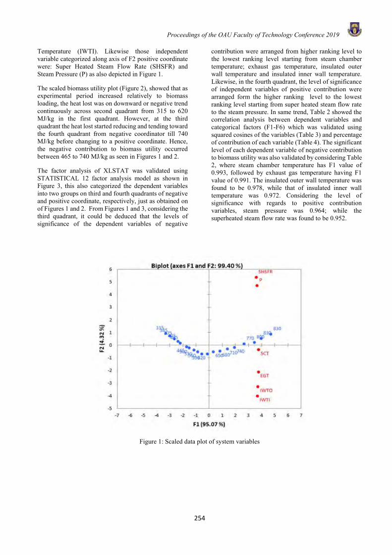
Proceedings of the OAU Faculty of Technology Conference 2019
254
Temperature (IWTI). Likewise those independent variable categorized along axis of F2 positive coordinate were: Super Heated Steam Flow Rate (SHSFR) and Steam Pressure (P) as also depicted in Figure 1.
The scaled biomass utility plot (Figure 2), showed that as experimental period increased relatively to biomass loading, the heat lost was on downward or negative trend continuously across second quadrant from 315 to 620 MJ/kg in the first quadrant. However, at the third quadrant the heat lost started reducing and tending toward the fourth quadrant from negative coordinator till 740 MJ/kg before changing to a positive coordinate. Hence, the negative contribution to biomass utility occurred between 465 to 740 MJ/kg as seen in Figures 1 and 2.
The factor analysis of XLSTAT was validated using STATISTICAL 12 factor analysis model as shown in Figure 3, this also categorized the dependent variables into two groups on third and fourth quadrants of negative and positive coordinate, respectively, just as obtained on of Figures 1 and 2. From Figures 1 and 3, considering the third quadrant, it could be deduced that the levels of significance of the dependent variables of negative
contribution were arranged from higher ranking level to the lowest ranking level starting from steam chamber temperature; exhaust gas temperature, insulated outer wall temperature and insulated inner wall temperature. Likewise, in the fourth quadrant, the level of significance of independent variables of positive contribution were arranged form the higher ranking level to the lowest ranking level starting from super heated steam flow rate to the steam pressure. In same trend, Table 2 showed the correlation analysis between dependent variables and categorical factors (F1-F6) which was validated using squared cosines of the variables (Table 3) and percentage of contribution of each variable (Table 4). The significant level of each dependent variable of negative contribution to biomass utility was also validated by considering Table 2, where steam chamber temperature has F1 value of 0.993, followed by exhaust gas temperature having F1 value of 0.991. The insulated outer wall temperature was found to be 0.978, while that of insulated inner wall temperature was 0.972. Considering the level of significance with regards to positive contribution variables, steam pressure was 0.964; while the superheated steam flow rate was found to be 0.952.
Figure 1: Scaled data plot of system variables
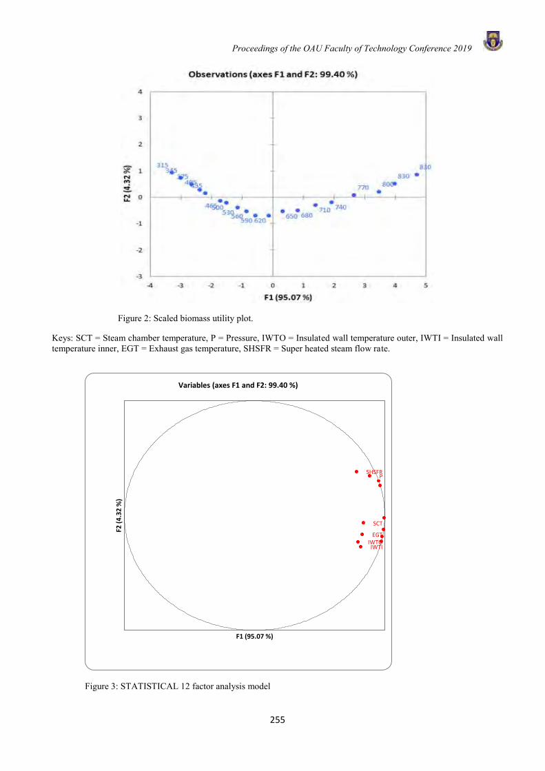
Proceedings of the OAU Faculty of Technology Conference 2019
255
Figure 2: Scaled biomass utility plot.
Keys: SCT = Steam chamber temperature, P = Pressure, IWTO = Insulated wall temperature outer, IWTI = Insulated wall temperature inner, EGT = Exhaust gas temperature, SHSFR = Super heated steam flow rate.
Figure 3: STATISTICAL 12 factor analysis model
SCT
P
IWTOIWTI
EGT
SHSFR
F2 (
4.3
2 %
)
F1 (95.07 %)
Variables (axes F1 and F2: 99.40 %)
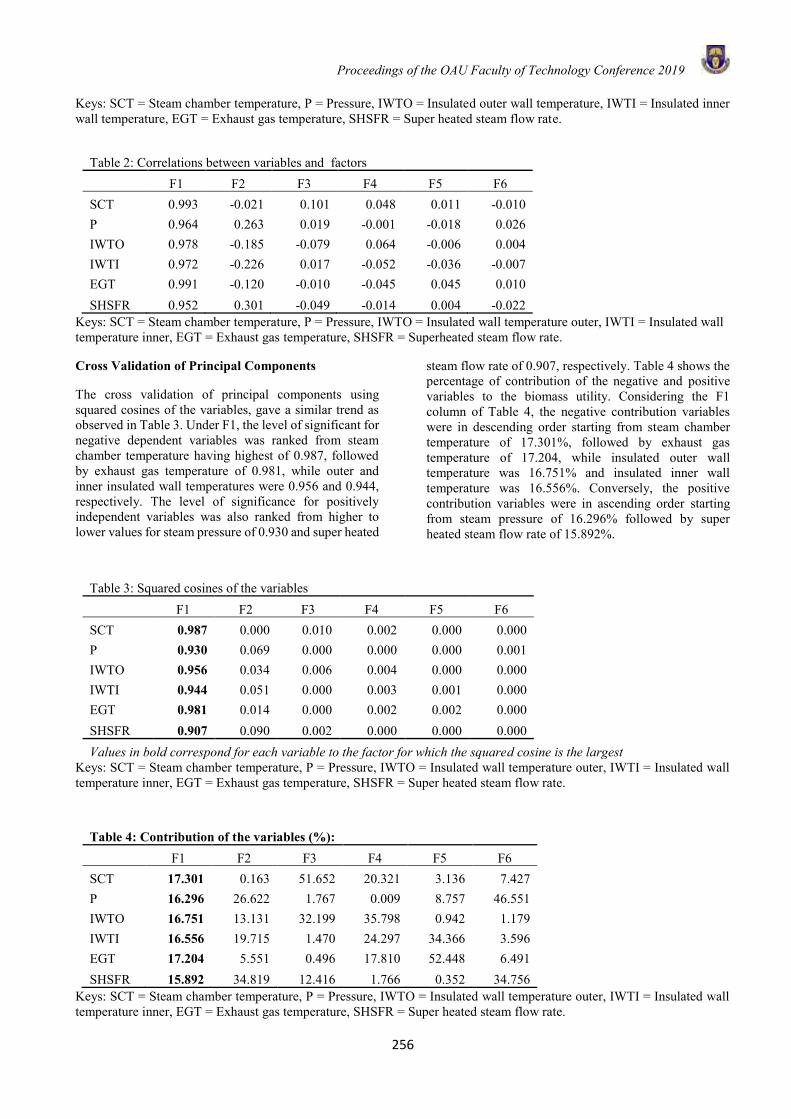
Proceedings of the OAU Faculty of Technology Conference 2019
256
Keys: SCT = Steam chamber temperature, P = Pressure, IWTO = Insulated outer wall temperature, IWTI = Insulated inner wall temperature, EGT = Exhaust gas temperature, SHSFR = Super heated steam flow rate.
Table 2: Correlations between variables and factors
F1 F2 F3 F4 F5 F6 SCT 0.993 -0.021 0.101 0.048 0.011 -0.010 P 0.964 0.263 0.019 -0.001 -0.018 0.026 IWTO 0.978 -0.185 -0.079 0.064 -0.006 0.004 IWTI 0.972 -0.226 0.017 -0.052 -0.036 -0.007 EGT 0.991 -0.120 -0.010 -0.045 0.045 0.010 SHSFR 0.952 0.301 -0.049 -0.014 0.004 -0.022
Keys: SCT = Steam chamber temperature, P = Pressure, IWTO = Insulated wall temperature outer, IWTI = Insulated wall temperature inner, EGT = Exhaust gas temperature, SHSFR = Superheated steam flow rate.
Cross Validation of Principal Components
The cross validation of principal components using squared cosines of the variables, gave a similar trend as observed in Table 3. Under F1, the level of significant for negative dependent variables was ranked from steam chamber temperature having highest of 0.987, followed by exhaust gas temperature of 0.981, while outer and inner insulated wall temperatures were 0.956 and 0.944, respectively. The level of significance for positively independent variables was also ranked from higher to lower values for steam pressure of 0.930 and super heated
steam flow rate of 0.907, respectively. Table 4 shows the percentage of contribution of the negative and positive variables to the biomass utility. Considering the F1 column of Table 4, the negative contribution variables were in descending order starting from steam chamber temperature of 17.301%, followed by exhaust gas temperature of 17.204, while insulated outer wall temperature was 16.751% and insulated inner wall temperature was 16.556%. Conversely, the positive contribution variables were in ascending order starting from steam pressure of 16.296% followed by super heated steam flow rate of 15.892%.
Table 3: Squared cosines of the variables
F1 F2 F3 F4 F5 F6 SCT 0.987 0.000 0.010 0.002 0.000 0.000 P 0.930 0.069 0.000 0.000 0.000 0.001 IWTO 0.956 0.034 0.006 0.004 0.000 0.000 IWTI 0.944 0.051 0.000 0.003 0.001 0.000 EGT 0.981 0.014 0.000 0.002 0.002 0.000 SHSFR 0.907 0.090 0.002 0.000 0.000 0.000 Values in bold correspond for each variable to the factor for which the squared cosine is the largest
Keys: SCT = Steam chamber temperature, P = Pressure, IWTO = Insulated wall temperature outer, IWTI = Insulated wall temperature inner, EGT = Exhaust gas temperature, SHSFR = Super heated steam flow rate.
Table 4: Contribution of the variables (%):
F1 F2 F3 F4 F5 F6 SCT 17.301 0.163 51.652 20.321 3.136 7.427 P 16.296 26.622 1.767 0.009 8.757 46.551 IWTO 16.751 13.131 32.199 35.798 0.942 1.179 IWTI 16.556 19.715 1.470 24.297 34.366 3.596 EGT 17.204 5.551 0.496 17.810 52.448 6.491 SHSFR 15.892 34.819 12.416 1.766 0.352 34.756
Keys: SCT = Steam chamber temperature, P = Pressure, IWTO = Insulated wall temperature outer, IWTI = Insulated wall temperature inner, EGT = Exhaust gas temperature, SHSFR = Super heated steam flow rate.
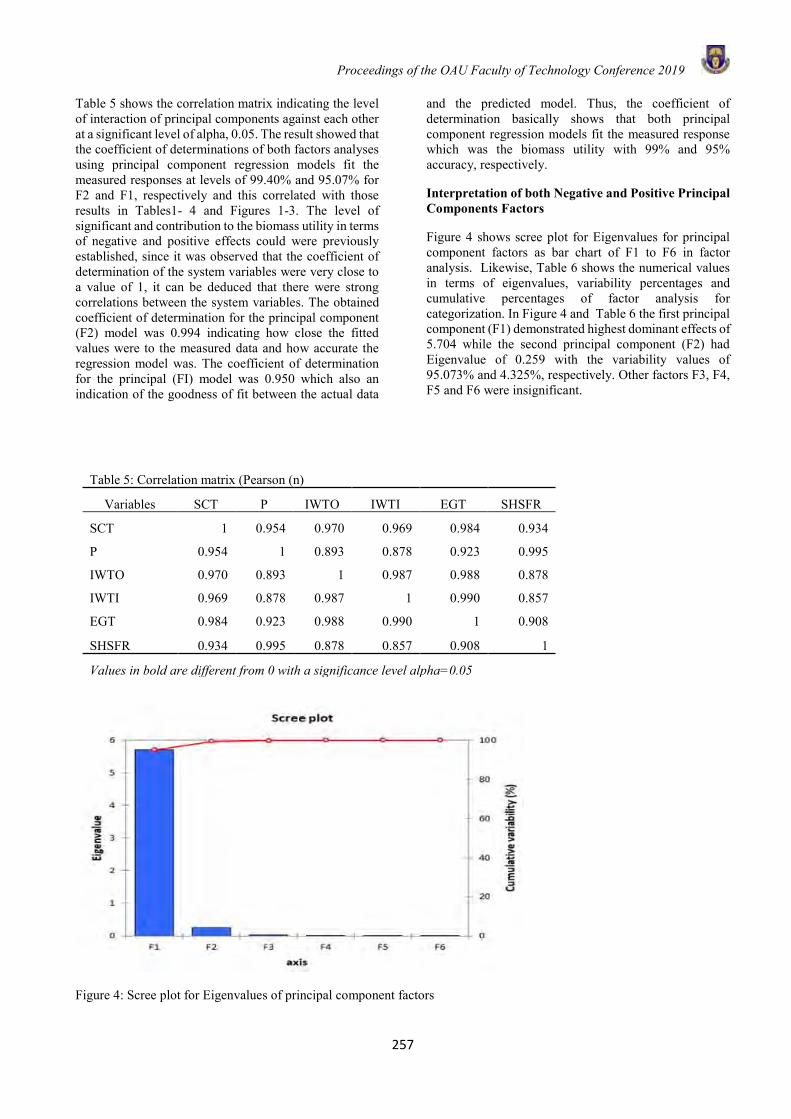
Proceedings of the OAU Faculty of Technology Conference 2019
257
Table 5 shows the correlation matrix indicating the level of interaction of principal components against each other at a significant level of alpha, 0.05. The result showed that the coefficient of determinations of both factors analyses using principal component regression models fit the measured responses at levels of 99.40% and 95.07% for F2 and F1, respectively and this correlated with those results in Tables1- 4 and Figures 1-3. The level of significant and contribution to the biomass utility in terms of negative and positive effects could were previously established, since it was observed that the coefficient of determination of the system variables were very close to a value of 1, it can be deduced that there were strong correlations between the system variables. The obtained coefficient of determination for the principal component (F2) model was 0.994 indicating how close the fitted values were to the measured data and how accurate the regression model was. The coefficient of determination for the principal (FI) model was 0.950 which also an indication of the goodness of fit between the actual data
and the predicted model. Thus, the coefficient of determination basically shows that both principal component regression models fit the measured response which was the biomass utility with 99% and 95% accuracy, respectively.
Interpretation of both Negative and Positive Principal Components Factors
Figure 4 shows scree plot for Eigenvalues for principal component factors as bar chart of F1 to F6 in factor analysis. Likewise, Table 6 shows the numerical values in terms of eigenvalues, variability percentages and cumulative percentages of factor analysis for categorization. In Figure 4 and Table 6 the first principal component (F1) demonstrated highest dominant effects of 5.704 while the second principal component (F2) had Eigenvalue of 0.259 with the variability values of 95.073% and 4.325%, respectively. Other factors F3, F4, F5 and F6 were insignificant.
Table 5: Correlation matrix (Pearson (n)
Variables SCT P IWTO IWTI EGT SHSFR
SCT 1 0.954 0.970 0.969 0.984 0.934
P 0.954 1 0.893 0.878 0.923 0.995
IWTO 0.970 0.893 1 0.987 0.988 0.878
IWTI 0.969 0.878 0.987 1 0.990 0.857
EGT 0.984 0.923 0.988 0.990 1 0.908
SHSFR 0.934 0.995 0.878 0.857 0.908 1
Values in bold are different from 0 with a significance level alpha=0.05
Figure 4: Scree plot for Eigenvalues of principal component factors
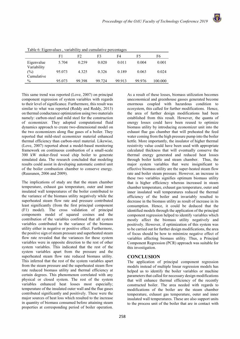
Proceedings of the OAU Faculty of Technology Conference 2019
258
Table 6: Eigenvalues , variability and cumulative percentages F1 F2 F3 F4 F5 F6
Eigenvalue 5.704 0.259 0.020 0.011 0.004 0.001 Variability (%) 95.073 4.325 0.326 0.189 0.063 0.024 Cumulative % 95.073 99.398 99.724 99.913 99.976 100.000
This same trend was reported (Love, 2007) on principal component regression of system variables with regards to their level of significance. Furthermore, this result was similar to what was reported (Reddy and Reddy, 2013) on thermal conductance optimization using two materials namely: carbon-steel and mild steel for the construction of economizer. They adopted computational fluid dynamics approach to create two-dimensional model on the two economizers along flue gases of a boiler. They reported that mild-steel economizer material enhanced thermal efficiency than carbon-steel material. Likewise, (Love, 2007) reported about a model-based monitoring framework on continuous combustion of a small-scale 300 kW stoker-fired wood chip boiler to generate simulated data. The research concluded that modeling results could assist in developing automatic control unit of the boiler combustion chamber to conserve energy. (Ruusunen, 2006 and 2009).
The implications of study are that the steam chamber temperature, exhaust gas temperature, outer and inner insulated wall temperatures of the boiler contributed to the variance of the biomass utility negatively while the superheated steam flow rate and pressure contributed least significantly (from the first principal component (F1) model). The cross validation of principal components model of squared cosines and the contribution of the variables confirmed that all system variables contributed to the variance of the biomass utility either in negative or positive effect. Furthermore, the positive sign of steam pressure and superheated steam flow rate revealed that the variances for these system variables were in opposite direction to the rest of other system variables. This indicated that the rest of the system variables apart from the pressure and the superheated steam flow rate reduced biomass utility. This inferred that the rest of the system variables apart from the steam pressure and the superheated steam flow rate reduced biomass utility and thermal efficiency at certain degrees. This phenomenon correlated with any physical or closed system. The rest of the system variables enhanced heat losses most especially; temperature of the insulated outer wall and the flue gases contributed significantly and positively. These were the major sources of heat loss which resulted to the increase in quantity of biomass consumed before attaining steam properties at corresponding period of boiler operation.
As a result of these losses, biomass utilization becomes uneconomical and greenhouse gasses generated become enormous coupled with hazardous condition to ecosystem, this called for further modifications. Hence, the area of further design modifications had been established from this result. However, the quanta of energy losses could have been reused to optimize biomass utility by introducing economizer unit into the exhaust flue gas chamber that will preheated the feed water coming from the high pressure pump into the boiler kettle. More importantly, the insulator of higher thermal resistivity value could have been used with appropriate calculated thickness that will eventually conserve the thermal energy generated and reduced heat losses through boiler kettle and steam chamber. Thus, the major system variables that were insignificant to effective biomass utility are the super-heated steam flow rate and boiler steam pressure. However, an increase in these two variables signifies optimum biomass utility that is higher efficiency whereas increased in steam chamber temperature, exhaust gas temperature, outer and inner insulated wall temperatures reduced the thermal efficiency of the boiler and invariably resulted to decrease in the biomass utility as result of increase in its consumption. Hence, it could be deduced that the identified models through the application of the principal component regression helped to identify variables which mostly affect the biomass utility negatively and positively. However, if optimization of this system was to be carried out for further design modifications, the area of focus should be how to minimize negative effect of variables affecting biomass utility. Thus, a Principal Component Regression (PCR) approach was suitable for this investigation.
CONCLUSION The application of principal component regression models instead of multiple linear regression models has helped us to identify the boiler variables or machine parameters that called for necessary design modifications that will enhance thermal efficiency of the recently constructed boiler. The area needed with regards to modifications of the boiler are the steam chamber temperature, exhaust gas temperature, outer and inner insulated wall temperatures. These are also support units to the process unit of the boiler that are in contact with
Proceedings of the OAU Faculty of Technology Conference 2019
259
the environment. This means that the whole boiler metallic structure should be housed with higher thermal resistivity insulator value for higher thermal efficiency. This can be accomplished by replacing the existing glass fibre with another insulator of higher thermal resistivity and employing appropriate design calculation to determine its optimum thickness. More importantly, an economizer should be introduced to preheat feed water before entering the kettle. Generally, steam generators should be re-calibrated on regular bases, likewise their thermal efficiency validated whether the lagging is efficient or otherwise. Empirically, from Table 4, the steam chamber temperature contributed negatively at higher percentage than other parameters, since there was no lagging material to conserve heat of conduction through outer wall of this chamber to the environment. Hence for further modification, appropriate insulation material and thickness should be installed to conserve heat content of the superheated steam generated. This will enhance positive biomass utility and eventually reduce cost of operation. Obviously, higher energy efficient system will ensure effective biomass utility. In the same trend, to reduce heat loss through flue gases, the permanent solution is to install an economizer that will pre-heat the feed water before entering into the kettle, thereby inhibiting heat losses which affect biomass utility negatively.
ACKNOWNLEGDEMENTS The authors wish to appreciate the facilities provided by the Department of Food Science and Technology, Faculty of Technology, Obafemi Awolowo University, Ile-Ife, Osun State, Nigeria toward the success of this research work.
REFERENCES Febrero, L., Granada, E., Regueiro, A., Míguez , J.L.,
Influence of Combustion Parameters on Fouling Composition after Wood Pellet Burning in a Lab-Scale Low-Power Boiler Energies. 8, 9794-9816; doi:10.3390/en8099794, 2015.
Heikki, L., Small-scale pellet boiler emissions-characterization and comparison to other combustion unit. Academic Dissertation of Faculty of Science and Forestry of the University of Eastern Finland Kuopio,. Pg. 1-13.
https://www.epa.gov/sites/production/files/documents/20090210panelseroutreachmeeting.pdf Google Scholar, 2014.
Lienhard IV, J. H., Lienhard V, J. H., Heat transfer textbook. Fourth edition, Phlogiston press Cambridge Massachusetts, Version 2.1 pg. 10-34, 2017.
Love, J., Process Automation Handbook: A Guide to Theory and Practice. London: Springer London, 2007.
Master, B. I., Chunangad, K. S., Pushpanathan, V., Fouling mitigation using helix-changer heat exchangers. Proceedings of the ECI Conference on Heat Exchanger Fouling and Cleaning:
Fundamentals and Applications, Santa Fe, USA,317–322, 2003.
Morakinyo, T. A., Bamgboye, A. I., “The Optimization of Operational Parameters of a Biomass Fire-in-tube Boiler Using Taguchi Design Method.” American Journal of Food Science and Technology, vol. 5, no. 5 167-175. doi: 10.12691/ajfst-5-5-1, 2017.
Morakinyo, T.A., Bamgboye, A. I., Optimization of Operation Parameters of a vertical sterilizer of Medium-Scale Oil Palm Mill Using Taguchi Method, Journal of Food Process Engineering, 40(5) DOI: 10.1111/JFPE.12453, 2016.
NCSS.com., ‘Principal Components Regression’. Available at:https://ncss-wpengine.netdna-ssl.com/wp-content/themes/ncss/pdf/Procedures/NCSS/Principal_Components_Regression.pdf (Accessed: 10 July 2018), 2018.
Ojolo, S. J., Orisaleye, J. I., Ismail, S.O., Abolarin, S.M., Technical potential of biomass energy in Nigeria. Ife Journal of Technology, 21 (2):60–65, 2012.
Orisaleye, J. I., Jekayinfa, S. O., Adebayo, A. O., Ahmed, N. A., Pecenka, R., Effect of densification variables on density of corn cob briquettes produced using a uniaxial compaction biomass briquetting press, Energy Sources, Part A: Recovery, Utilization, and Environmental Effects, doi: 10.1080/15567036.2018.1516007, 2018.
Oyedepo, S.O., Energy Efficiency and Conservation Measures: Tools for Sustainable Energy Development in Nigeria. International Journal of Energy Engineering. IJEE, 2(3):86-98, 2012.
Panel, S. E. R., Outreach Meeting, Combined Rulemaking for Industrial, Commercial, and Institutional Boilers and Process Heaters at Major Sources of HAP and Industrial Boilers and Commercial and Institutional Boilers at Area Sources. https://www.epa.gov/sites/production/files/documents/20090210panelseroutreachmeeting.pdf Google Scholar, 2009.
Reddy, K. S. K., Reddy, B. V., Performance of boiler and to improving the boiler efficiency using Cfd Modeling. Journal of Mechanical and Civil Engineering, 8(6): 25-29, 2013.
Ruusunen, M., Monitoring of small-scale biomass combustion processes. Report Series A 29. March 2006. Department of Process and Environmental Engineering, Control Engineering Laboratory. ISBN 951-42-8027-X. ISSN 1238-9390 FIN-90014, University of Oulu,. Finland: 1-34, 2006a.
Ruusunen, M., Modelling and control of small-scale biomass combustion for emission reduction. In: Paukkeri, A.; Ylä-Mella, J. and Pongrácz, E. (eds.) Energy research at the University of Oulu. Proceedings of the EnePro conference, June 3rd, 2009, University of Oulu, Finland. Kaleva print, Oulu,. ISBN 978-951-42-9154-8: 75-78, 2009.

Proceedings of the OAU Faculty of Technology Conference 2019
260
Shah, S., Adhyaru, D. MBoiler Efficiency Analysis using Direct Method. In: International Conference on Current Trends in Technology. IEEE Press, New York. 1–5, 2010.
UNIDO., Manual for industrial steam systems assessment and optimization. https://www unido.org/site/SSO-manual-print-final-20161109-one-pgev2pdf, 2016.
Wang, W., Chen, L., Han, X., Ge, Z., Wang, S., Modelling and Application of Principal Component Analysis in Industrial Boiler. Advances in Neural Networks Springer International Publishing Switzerland,. 395–404. DOI: 10.1007/978-3-319-12436-0_44, 2014.
Yang, J., Oh, S. R., Liu, W., Optimization of shell and tube heat exchangers using a general design approach motivated by contractual theory. International Journal of heat and mass transfer, (77): 1144 -1154, 2014.
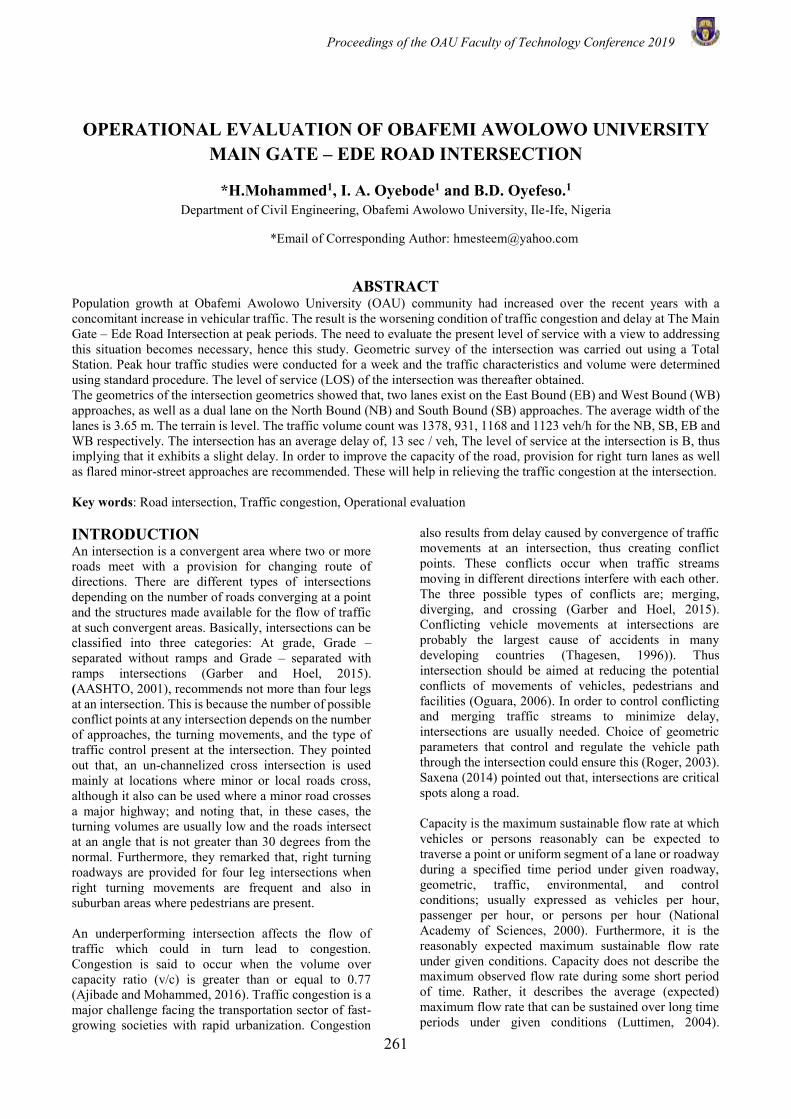
Proceedings of the OAU Faculty of Technology Conference 2019
261
OPERATIONAL EVALUATION OF OBAFEMI AWOLOWO UNIVERSITY MAIN GATE – EDE ROAD INTERSECTION
*H.Mohammed1, I. A. Oyebode1 and B.D. Oyefeso.1 Department of Civil Engineering, Obafemi Awolowo University, Ile-Ife, Nigeria
*Email of Corresponding Author: [email protected]
ABSTRACT Population growth at Obafemi Awolowo University (OAU) community had increased over the recent years with a concomitant increase in vehicular traffic. The result is the worsening condition of traffic congestion and delay at The Main Gate – Ede Road Intersection at peak periods. The need to evaluate the present level of service with a view to addressing this situation becomes necessary, hence this study. Geometric survey of the intersection was carried out using a Total Station. Peak hour traffic studies were conducted for a week and the traffic characteristics and volume were determined using standard procedure. The level of service (LOS) of the intersection was thereafter obtained. The geometrics of the intersection geometrics showed that, two lanes exist on the East Bound (EB) and West Bound (WB) approaches, as well as a dual lane on the North Bound (NB) and South Bound (SB) approaches. The average width of the lanes is 3.65 m. The terrain is level. The traffic volume count was 1378, 931, 1168 and 1123 veh/h for the NB, SB, EB and WB respectively. The intersection has an average delay of, 13 sec / veh, The level of service at the intersection is B, thus implying that it exhibits a slight delay. In order to improve the capacity of the road, provision for right turn lanes as well as flared minor-street approaches are recommended. These will help in relieving the traffic congestion at the intersection. Key words: Road intersection, Traffic congestion, Operational evaluation INTRODUCTION An intersection is a convergent area where two or more roads meet with a provision for changing route of directions. There are different types of intersections depending on the number of roads converging at a point and the structures made available for the flow of traffic at such convergent areas. Basically, intersections can be classified into three categories: At grade, Grade – separated without ramps and Grade – separated with ramps intersections (Garber and Hoel, 2015). (AASHTO, 2001), recommends not more than four legs at an intersection. This is because the number of possible conflict points at any intersection depends on the number of approaches, the turning movements, and the type of traffic control present at the intersection. They pointed out that, an un-channelized cross intersection is used mainly at locations where minor or local roads cross, although it also can be used where a minor road crosses a major highway; and noting that, in these cases, the turning volumes are usually low and the roads intersect at an angle that is not greater than 30 degrees from the normal. Furthermore, they remarked that, right turning roadways are provided for four leg intersections when right turning movements are frequent and also in suburban areas where pedestrians are present. An underperforming intersection affects the flow of traffic which could in turn lead to congestion. Congestion is said to occur when the volume over capacity ratio (v/c) is greater than or equal to 0.77 (Ajibade and Mohammed, 2016). Traffic congestion is a major challenge facing the transportation sector of fast-growing societies with rapid urbanization. Congestion
also results from delay caused by convergence of traffic movements at an intersection, thus creating conflict points. These conflicts occur when traffic streams moving in different directions interfere with each other. The three possible types of conflicts are; merging, diverging, and crossing (Garber and Hoel, 2015). Conflicting vehicle movements at intersections are probably the largest cause of accidents in many developing countries (Thagesen, 1996)). Thus intersection should be aimed at reducing the potential conflicts of movements of vehicles, pedestrians and facilities (Oguara, 2006). In order to control conflicting and merging traffic streams to minimize delay, intersections are usually needed. Choice of geometric parameters that control and regulate the vehicle path through the intersection could ensure this (Roger, 2003). Saxena (2014) pointed out that, intersections are critical spots along a road. Capacity is the maximum sustainable flow rate at which vehicles or persons reasonably can be expected to traverse a point or uniform segment of a lane or roadway during a specified time period under given roadway, geometric, traffic, environmental, and control conditions; usually expressed as vehicles per hour, passenger per hour, or persons per hour (National Academy of Sciences, 2000). Furthermore, it is the reasonably expected maximum sustainable flow rate under given conditions. Capacity does not describe the maximum observed flow rate during some short period of time. Rather, it describes the average (expected) maximum flow rate that can be sustained over long time periods under given conditions (Luttimen, 2004).
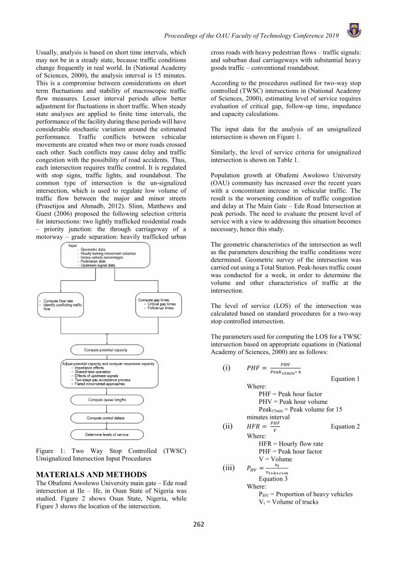
Proceedings of the OAU Faculty of Technology Conference 2019
262
Usually, analysis is based on short time intervals, which may not be in a steady state, because traffic conditions change frequently in real world. In (National Academy of Sciences, 2000), the analysis interval is 15 minutes. This is a compromise between considerations on short term fluctuations and stability of macroscopic traffic flow measures. Lesser interval periods allow better adjustment for fluctuations in short traffic. When steady state analyses are applied to finite time intervals, the performance of the facility during these periods will have considerable stochastic variation around the estimated performance. Traffic conflicts between vehicular movements are created when two or more roads crossed each other. Such conflicts may cause delay and traffic congestion with the possibility of road accidents. Thus, each intersection requires traffic control. It is regulated with stop signs, traffic lights, and roundabout. The common type of intersection is the un-signalized intersection, which is used to regulate low volume of traffic flow between the major and minor streets (Prasetijoa and Ahmadb, 2012). Slinn, Matthews and Guest (2006) proposed the following selection criteria for intersections: two lightly trafficked residential roads – priority junction: the through carriageway of a motorway – grade separation: heavily trafficked urban
cross roads with heavy pedestrian flows – traffic signals: and suburban dual carriageways with substantial heavy goods traffic – conventional roundabout. According to the procedures outlined for two-way stop controlled (TWSC) intersections in (National Academy of Sciences, 2000), estimating level of service requires evaluation of critical gap, follow-up time, impedance and capacity calculations. The input data for the analysis of an unsignalized intersection is shown on Figure 1. Similarly, the level of service criteria for unsignalized intersection is shown on Table 1. Population growth at Obafemi Awolowo University (OAU) community has increased over the recent years with a concomitant increase in vehicular traffic. The result is the worsening condition of traffic congestion and delay at The Main Gate – Ede Road Intersection at peak periods. The need to evaluate the present level of service with a view to addressing this situation becomes necessary, hence this study.
Figure 1: Two Way Stop Controlled (TWSC) Unsignalized Intersection Input Procedures MATERIALS AND METHODS The Obafemi Awolowo University main gate – Ede road intersection at Ile – Ife, in Osun State of Nigeria was studied. Figure 2 shows Osun State, Nigeria, while Figure 3 shows the location of the intersection.
The geometric characteristics of the intersection as well as the parameters describing the traffic conditions were determined. Geometric survey of the intersection was carried out using a Total Station. Peak-hours traffic count was conducted for a week, in order to determine the volume and other characteristics of traffic at the intersection. The level of service (LOS) of the intersection was calculated based on standard procedures for a two-way stop controlled intersection. The parameters used for computing the LOS for a TWSC intersection based on appropriate equations in (National Academy of Sciences, 2000) are as follows:
(i) 𝑃𝐻𝐹 = 𝑃𝐻𝑉
𝑃𝑒𝑎𝑘15𝑚𝑖𝑛∗ 4
Equation 1 Where:
PHF = Peak hour factor PHV = Peak hour volume Peak15min = Peak volume for 15
minutes interval (ii) 𝐻𝐹𝑅 =
𝑃𝐻𝐹
𝑉 Equation 2
Where: HFR = Hourly flow rate PHF = Peak hour factor V = Volume
(iii) 𝑃𝐻𝑉 =𝑣𝑡
𝑣𝑡+𝑏+𝑐+𝑚
Equation 3 Where: PHV = Proportion of heavy vehicles Vt = Volume of trucks

Proceedings of the OAU Faculty of Technology Conference 2019
263
Vt+b+c+m = Volume of trucks, buses, cars and motorcycles
(iv) 𝑡𝑐,𝑥 = 𝑡𝑐,𝑏𝑎𝑠𝑒 + 𝑡𝑐,𝐻𝑉𝑃𝐻𝑉 + 𝑡𝑐,𝐺𝐺 − 𝑡𝑐,𝑇 −
𝑡3,𝐿𝑇 Equation 4 Where:
tc,x = critical gap for movement x (s),
tc,base = base critical gap from Table 2
tc,HV = adjustment factor for heavy vehicles (1.0) for two-lane major streets and 2.0 for four-lane major streets) (s),
PHV = Proportion of heavy vehicles
tc,G = adjustment factor for grade (0.1 for Movements 9 and 12 and 0.2 for Movements 7. 8, 10, and 11) (s),
G = percent grade divided by 100,
tc,T = adjustment factor for each part of a two-stage gap acceptance process (1.0 for first or second stage; 0.0 if only one stage) (s), and
t3,LT = adjustment factor for intersection geometry (0.7 for minor-street left-turn movement at three-leg intersection; 0,0 otherwise) (s).
(v) 𝑡𝑓 = 𝑡𝑓𝑏𝑎𝑠𝑒 + 𝑡𝑓𝐻𝑉 ∗ 𝑃𝐻𝑉 Equation 5 Where:
tf = follow up time
tfbase = base follow up time: 2.2 for left turn from major, 3.3 for right turn from minor, 4.0 for through traffic on minor and 3.5 for left turn from minor (s)
PHV = Proportion of heavy vehicles
(vi) 𝑐𝑝,𝑥 = 𝑣𝑐,𝑥𝑒−𝑣𝑐,𝑥𝑡𝑐,𝑥/3600
1−𝑒−𝑣𝑐,𝑥𝑡𝑓,𝑥/3600
Equation 6 Where:
cp,x = potential capacity of minor
movement x (veh/h),
vc,x = conflicting flow rate for movement x
(veh/h),
tc,x = critical gap (i.e., the minimum time
that allows intersection entry for one
minor-stream vehicle) for minor
movement x (s), and
tf,x = follow-up time
(vii) 𝑐𝑆𝐻 =∑ 𝑣𝑦𝑦
∑ (𝑣𝑦
𝑐𝑚,𝑦)𝑦
Equation 7
Where:
CSH = capacity of the shared lane (veh/h)
Vy = flow rate of the y movement in the subject shared lane (veh/h), and
Cm,y = movement capacity of the y movement in the subject shared lane (veh/h).
(viii) 𝑄95 = 900𝑇 [𝑣𝑥
𝑐𝑚,𝑥− 1 +
√((𝑣𝑥
𝑐𝑚,𝑥− 1)
2 (3600
𝑐𝑚,𝑥)(
𝑣𝑥𝑐𝑚,𝑥
)
150𝑇)] (
𝑐𝑚,𝑥
3600)
Equation 8 Where:
Q95 = 95TH- percentile queue (veh),
Vx = flow rate for movement x (veh/h),
Cm,x = capacity of movement x (veh/h), and
T = analysis time period (h) (T = 0.25 for a 15-min period).
(ix) 𝑑 =3600
𝑐𝑚,𝑥+ 900𝑇 [
𝑣𝑥
𝑐𝑚,𝑥− 1 +
√((𝑣𝑥
𝑐𝑚,𝑥− 1)
2
+(3600
𝑐𝑚,𝑥)(
𝑣𝑥𝑐𝑚,𝑥
)
450𝑇)] + 5
Equation 9 Where:
d = control delay (s/veh),
vx = flow rate for movement x (veh/h),
cm,x = capacity of movement x (veh/h), and
T = analysis time period (h) (T = 0.25 for a 15-
min analysis.
Proceedings of the OAU Faculty of Technology Conference 2019
264
Table 1: Level –of– Service Criteria for TWSC Intersections
Level of Service Average Control Delay (s/veh)
A 0-10 B > 10 – 15 C > 15 – 25 D > 25 – 35 E > 35 – 50 F > 50
Source: Highway Capacity Manual (2000).
Figure 2: Map of Nigeria showing Osun States
Source:
http://www.ngex.com/nigeria/places/states/osun.htm
Figure 3: Intersection Location North
RESULTS AND DISCUSSION The intersection geometrics show that the Obafemi Awolowo University Main Gate – Ede road intersection consists of four legs namely: OAU Campus Gate
approach (North Bound), Ibadan road pedestrian bridge approach (South Bound), Mayfair road approach (East Bound) and Ede road approach (West Bound) as shown in Figure 4. The road was built as a flexible pavement using asphaltic concrete. The condition of all the legs of the intersection can be considered as good as there is no visible road defect on the main carriageway. The vehicles plying the road are: passenger cars, motorcycles, buses, and trucks.
The Campus Gate and the Ibadan Road Pedestrian Bridge legs of the intersection serve as the minor or stop-controlled approaches while the Ede road and Mayfair road serve as the major street/approach.
Furthermore, there are two lanes on the East Bound (EB) and West Bound (WB) approaches, and a dual lane on the North Bound (NB) and South Bound (SB) approaches with an average lane width of 3.65 m. The terrain is level with a parking facility on the North Bound approach, and an average turning angle of 95°. The traffic volume count gave a total of 1378, 931veh/hr for NB and SB approaches respectively. Similarly, there was a total of 1168 and 1123 veh/hr for EB and WB traffic respectively. The highest traffic on the NB approach as shown in the intersection summary sheets in Figure 5 and Figure 6 aptly reflects that the intersection is typical of academic community which is a traffic generating centre. The traffic movements 7, 8 and 9 have queue lengths of 3.34 and 1.78 metres and control delay of 12.94 and 10.31 sec respectively which puts the level of service at B. Similarly, traffic movements 10, 11 and 12 have queue lengths of 6.20 and 4.66 metres and control delay of 21.52 and 15.94 seconds and therefore termed as operating at LOS: C. The movements 1 and 4 have a queue length of 0.55 and 0.21 metres and control delay of 9.46 and 8.69 seconds respectively corresponding to LOS A. Therefore, the average intersection delay is, 13 sec / veh, which put the overall level of service of the intersection at B, thus implying that there is a slight delay at the intersection which could be attributed to its inadequate geometrics.
Figure 4: Intersection Configuration

Proceedings of the OAU Faculty of Technology Conference 2019
265
Figure 5: Intersection Traffic Volume Summary Sheet for Peak Morning Hours
Figure 6: Intersection Traffic Volume Summary Sheet for Peak Evening Hours
CONCLUSION The operational evaluation of the Obafemi Awolowo University Main gate – Ede road intersection was carried out. The result of the survey of the geometry of the intersection showed that there was no provision for storage lanes on all the four approaches; thus, a contributory factor to the reduced capacity of the intersection. From the traffic data obtained and analysed, it can be concluded that the Campus Gate approach has the highest traffic, being the destination of majority of the traffic movements at the intersection originating from various parts of Ile-Ife and beyond. The overall Level of Service (L.O.S.) for the intersection is B. This implies that there is a slight delay at the intersection. The provision of right turn lanes is recommended for channelizing movements on the right turn so as to
reduce the delay experienced by other movements accessing the intersection. This will help in relieving the traffic congestion at the intersection. REFERENCES
AASHTO. (2001). A Policy on Geometric Design of Highways and Streets (Fourth). Retrieved from www.transportation.org Ajibade, M.and Mohammed, H. (2016). Operational Performance Evaluation of Post Office – Teaching Hospital road, Ile - Ife, Nigeria. Civil and Environmental Research, 8(7), 18–27. Garber, N. J.and Hoel, N. A. (2015). Traffic and Highway Engineering. Cengage Learning, Stamford, USA. Luttimen, R. T. (2004). Capacity and Level of Service at Finnish Unsignalized Intersections. Helsinki: Finnra Reports. National Academy of Sciences. (2000). Highway Capacity Manual. Transportation Research Board. Oguara, T. M. (2006). Highway Engineering. Lagos: Malthouse Press Limited. Prasetijoa, J.and Ahmadb, H. (2012). Capacity Analysis of Unsignalized Intersection Under Mixed Traffic Conditions. Procedia - Social and Behavioral Sciences, 43, 135–147. Roger, M. (2003). Highway Engineering (1st ed.). USA: Blackwell Publishing. Saxena, S. C. (2014). Highway and Traffic Engineering. New Delhi, India: CBS Publishers and Distributors. Slinn, M., Matthews, P.and Guest, P. (2006). Traffic Engineering Design. New Delhi, India: Elsevier. Thagesen, B. (1996). Highway and Traffic Engineering in Developing Countries. London: E and FN Spon.
Proceedings of the OAU Faculty of Technology Conference 2019
266
OPTIMIZATION OF BIODIESEL PRODUCTION FROM KHAYA
SENEGALENSIS OIL USING HETEROGENEOUS CATALYST
E. E. Onojowho1, S. O. Obayopo*1 and A. A. Asere1
1 Department of Mechanical Engineering, Obafemi Awolowo University, Ile-Ife, Nigeria
* Email of Corresponding Author: [email protected]
ABSTRACT Global concerned for an ecofriendly environment and upholding minimal biodiesel production cost simultaneously has prompted the use of organic wastes as heterogeneous catalyst for its production. In this work, response surface methodology (RSM) was used to optimize the production of biodiesel through a two-step transesterification process. The extracted Khaya senegalensis oil (KSO) possessed a high free fatty acid (FFA) value of 3.10 % which was reduced to 0.329 % using H2SO4 processed at 60 min reaction time, 60 ˚C temperature and a methanol to oil ratio of 2.25:1 (mol/mol). A calcined plantain peels (CPP) heterogeneous catalyst produced at 700 ˚C for 3.5 h was characterized and was found to contain potassium, sodium, calcium, magnesium, iron, manganese and phosphorus which was used for the transesterification to obtain Khaya senegalensis oil methyl esters (KSOME). A 97.98 wt% optimal KSOME yield was attained from a central composite design (CCD) using a quadratic model at a methanol to oil ratio of 9:1 (vol/vol), 2.5 (wt%) catalyst loading, 40 min reaction time and 65 °C constant temperature condition which was validated at 95.875 (wt%). KSOME produced met the international ASTM D6751 and DIN EN 14214 biodiesel standard specification hence, it is projected a good prospect for biodiesel production.
Keywords: Optimization, Heterogeneous catalyst, Biodiesel, Khaya senegalensis oil
INTRODUCTION Biodiesel production from biomass and wastes has become a subject of attention for most economies in the global quest for alternative energy sources to argument world energy reserves. Previous works focused on maximizing underutilized non-edible materials in biodiesel production with the view to reducing dependency on fossil fuels and price hike in many regions. Biodiesel apart from being renewable generally have good; lubricity, miscibility with conventional fuels, and low toxicity (Moser, 2009). Researches were delved on the potentials of some edible oil seeds (Ogunsuyi, 2015; Rachimoellah et al., 2009; Shote et al., 2009) though it has aroused controversy on domestic feedstock versus energy-economic driven development preference (Gui et al., 2008). In this regard, many non-edible oil seeds have been explored (Betiku et al., 2017; Junaid et al., 2014; SandeepKumar et al., 2015; Vivek and Gupta, 2004; Ying-Zhi et al., 2016). The use of used cooking oil (Mohammed and Bhargavi, 2015) have also been reported, while wood ash (Meeta et al., 2012), sea sand (Muciño et al., 2014), plantain peel, (Betiku and Ajala, 2014), shells and bones (Farooq and Ramli, 2015; Roschat et al., 2016) have been documented for heterogeneous catalyst production. Catalyst reusability, non-ediblity, cheap production cost, and waste conversion in environmental management are the significant pulls heterogeneous catalyst exacts in biodiesel production (Vicente and Mart, 2004). To strengthen the aforementioned advantages, investigations have been made in optimization study of oil extraction and transesterification yield with different
catalyst through various techniques and designs with the view of industrial profitability. Bhoopendra et al., (2017) reported using Taguchi design, Oyelade et al., (2017) used the D-optimal design, CCD was explored by Alok et al. (2007), and Betiku et al. (2017), while the comparison of Box-Behnken with Artificial neural network and genetic algorithm designs was investigated by Betiku and Ajala (2014) and Etim et al. (2018). Khaya senegalensis also known as African Mahogany, Ogonwo among the Yoruba’s (Orwa, 2009), Madachi for the Hausa’s (Blench and Dendo, 2007) is available in good quantity within these zones of Nigeria and is also called Ono in Igbo. This study is focused on determining the best biodiesel production condition from KSO using the CPP catalyst as well as characterizing the KSOME and the catalyst.
MATERIALS AND METHODS Materials African mahogany seeds of 2.2kg net weight was obtained from the Forest Research Institute, Ibadan. The plantain peels were obtained from restaurants on Obafemi Awolowo University campus Ile-Ife. All reagents used were analytical grade BDH Chemicals Ltd., Poole England and GFS Chemicals, Inc., Columbus. Methods
ii Khaya senegalensis oil (KSO) extraction
Proceedings of the OAU Faculty of Technology Conference 2019
267
The seeds were decorticated, dried and grinded for oil extraction using the chemical method in 250ml Soxhlet apparatus with n-Hexane. The seed granules were charged in a 24cm diameter thimble and into soxhlet which is fitted on 500ml flat-bottom flask. A condenser was fitted on soxhlet and everything was stand on a water-bath heating mantle whose temperature maintained 70 to 90 °C for a complete setup. The oil was separated from the refluxed n-Hexane after 9 h.
iii Preparation of calcined plantain peels (CPP) Combination of ripe and over-ripe peels were washed for 5 times with distilled water, chopped into bits, sun dried to crispy and opened-air burnt before grinding into fine power. The powered peel was charged into a furnace (Carbolite – Parsons Lane, Hope Valley, England. Model S33 6RB) for calcination at 700 °C for 3.5 h and CPP obtained was stored in air-tight bottle.
iv Esterification step of KSOME production This oil pretreatment step was necessary since the initial % FFA of the KSO of 3.10 is higher than the acceptable 1-2 % (Knothe et al., 2005) for good transesterification reaction. A 100g of oil was heated to 50 °C before charging with 225g methanol and 5g H2SO4 catalyst was allowed to react for 60 min at 60-65 °C temperature range. The was terminated after 60 min, esters were separated from the mixture after standing for 7 h in a separating funnel. This triplicate reaction yields a 0.329 % FFA and 95.70 % conversion for the transesterification step.
v A rotatable fractional CCD experiment The transesterification was pursued through a rotatable fractional CCD of 3factor, 5level coded as shown in Table 1 using RSM to generate 15 experimental runs on Design-Expert version 10 (Stat-Ease Inc., Minneapolis, MN, USA) software. Methanol to oil ratio (X1), catalyst loading (X2) and reaction time (X3) were the significant factors of interest as report in literature as well. The percentage yield was predicted from the second-order polynomial quadratic equation (1) to get the optimum model equation (2). Where
𝐲 = 𝛃𝟎 + ∑𝛃𝐢𝐗𝐢
𝐤
𝐢=𝟏
+ ∑𝛃𝐢𝐢𝐗𝐢𝟐
𝐤
𝐢=𝟏
+ ∑ ∑ 𝛃𝐢𝐣𝐗𝐢𝐗𝐣
𝐤
𝐢<𝐣=𝟐
+ 𝛆 i.
y is the yield, βi is the first-order model coefficients of main effects, βii stands for quadratic coefficients of quadratic effects, βij is the interactive effects coefficient for interacting effects, ε is a random error and i, j, and k are 1,2,3, …, n.
𝑦 = 0.8143 + 10.3561𝑋1 + 29.5997𝑋2
+ 0.9752𝑋3 − 0.5365𝑋1𝑋2
+ 0.0366𝑋1𝑋3
− 0.2319𝑋2𝑋3 − 0.6257𝑋12
− 3.4911𝑋22 − 0.0102𝑋3
2
ii
vi Optimized KSOME transesterification reaction step
Following the generated design from Table 1, a 12.26 ± 0.1 cm3 volume was held constant for all runs, measured
into a 500ml three-necked round-bottom flask with a corresponding volume of methanol for a run. This mixture was heated to 65 ° C before adding the corresponding quantity of catalyst and the time was started with the temperature maintained.
Table 7: Independent factors for the optimized
transesterification of KSOME on CCD FACTOR UNIT CODED FACTOR LEVELS
−𝜶 −𝟏 0 +𝟏 +𝜶 Methanol : Oil (X1)
vol/vol 4.7574 6 9 12 13.2426
Catalyst loading (X2)
% wt 1.0858 1.5 2.5 3.5 3.9142
Reaction time (X3)
min 11.7157 20 40 60 68.2843
IKA C-MAG HS 4 heating mantle and inbuilt magnetic stirrer at a maintained 1.5 stirring speed was used. At the end of the reaction time the mixture was separated into KSOME, glycerine and CPP phases with a centrifuge at 8000 rpm for 10 min before pouring into a separating funnel to stand for 15 min. KSOME obtained was purified with distilled water of 55 ° C to eliminate residues till the water is colourless (Van Gerpen et al., 2004) as shown in Figure 1, dehydration was necessary with sodium sulphate. KSOME yield is therefore calculated with equation (3) and the process repeated for all runs. The run bearing the highest as reflected in Table 2 was used in validation through mass production of KSOME.
% yield = weight of biodiesel
weight of oil used × 100% ii.
vi. Characterization of oil, KSOME and CPP The vital physical and chemical properties of extracted oil and KSOME were experimentally determined in accordance with the Association of Official Analytical Chemists (AOAC, 1995) standard methods for percentage oil content yield, acid value, iodine value, peroxide value, saponification value, density, surface tension, viscosity. Cloud point was through ASTM D 5773 method, pour point by ASTM D 97-96a method, open cup method of ASTM D 93 for smoke and flash points, ASTM D 613 and ASTM D 1997 method for cetane number and higher heating value respectively. A gram weight of CPP was used in 50 ml3 of solute for elemental composition study using atomic absorption spectroscopy (AAS) method on Aanalyst 400, Perion Eleanor, Singapore 2010 while absorption method was also used in Fourier Transform Infrared (FT-IR) to determine the active functional group of the CPP on Cary 630 Agilent, U.K.
RESULTS AND DISCUSSION The optimal production result presented in Table 2 indicates agreement with existing literature that the factors investigated in this work are significant production factors, presenting an optimum yield of 97.98 wt.% which was validated under created constraints methanol to oil ratio of 9:1 vol/vol, 2.5 wt.% catalyst loading and 40 min reaction time condition for the factors
Proceedings of the OAU Faculty of Technology Conference 2019
268
yielding 95.875 wt.% for mass production. This met the objective of optimal KSOME yield in the production.
(a)
(b)
Figure 1: (a) Separated phased KSOME and glycerol. (b) Purified KSOME phased with water underneath.
Analysis of the model for KSOME production ANOVA test result (Table 3) displayed a validation of the chosen model at 95 % confidence level with 0.0012 model p-value, accurately predicted that 0.12 % chances of noise existed at the model implementation. At the same confidence level was obtained 0.2327 p-value insignificant lack of fit, which was desired. In addition, regression equation R2 of 0.9785 greater than the least expected 0.80 (Joglekar and May, 1987) for a good fit means the model explained 97.85 % response relationships between yields and varying reacting conditions of Table 2 and was in agreement with Chin et al. (2009) result. The residual demonstrates a good relationship between the predicted and actual yield values as strengthen by 1.79 % coefficient of variance (C.V.) which is within the require less than 10 % for a good regression coefficient demonstrated in Figure 2. P-values greater than 0.05 are insignificant at 95 % confidence level hence X1, X2X3, 𝑋1
2, 𝑋22 and 𝑋3
2 factors are significant just as the model is. The F-values can be
used to present a contribution order of each factors to the reactions where X1X2 indicated as the lowest F-value is the least. A three dimensional expression of the factors interactive effects on yield is demonstrated in Figure 3, pointing that an increase in X3 beyond 40 min will
Table 8: Rotatable fractional CCD KSOME optimal production
Run order
X1 X2 X3 Actual KSOME Yield
Predicted KSOME Yield
Residual
vol/vol % wt.
min % wt. % wt.
1 0 0 −𝛼 91.16 90.54 0.6244 2 +𝛼 0 0 82.13 81.51 0.6244 3 0 −𝛼 0 92.51 91.89 0.6244 4 0 0 0 95.98 96.10 −0.1178 5 −𝛼 0 0 88.79 88.17 0.6244 6 0 0 0 95.44 96.10 −0.6578 7 0 0 0 95.94 96.10 −0.1578 8 0 +𝛼 0 86.97 86.35 0.6244 9 −1 −1 −1 84.37 84.99 −0.6244 10 0 0 0 97.98 96.10 1.88 11 −1 1 1 75.6 76.22 −0.6244 12 0 0 +𝛼 85.95 85.33 0.6244 13 0 0 0 93.9 96.10 −2.20 14 1 1 −1 80.63 81.25 −0.6244 15 1 −1 1 88.47 89.09 −0.6244
transmit a negative yield response with X2 at constant X1 on Figure 3(c). However, a decreasing of X3 and increasing X2 will favour KSOME yield.
Figure 2: Plot of predicted versus actual KSOME yields
Fuel physicochemical properties A compares of investigated properties with exiting literature on the same seed in Table 4, divulged some splashy differences in cetane number, flash point, cloud point and pour point which may be due to cultivation and geographical variation effects on seed (Moser, 2009).
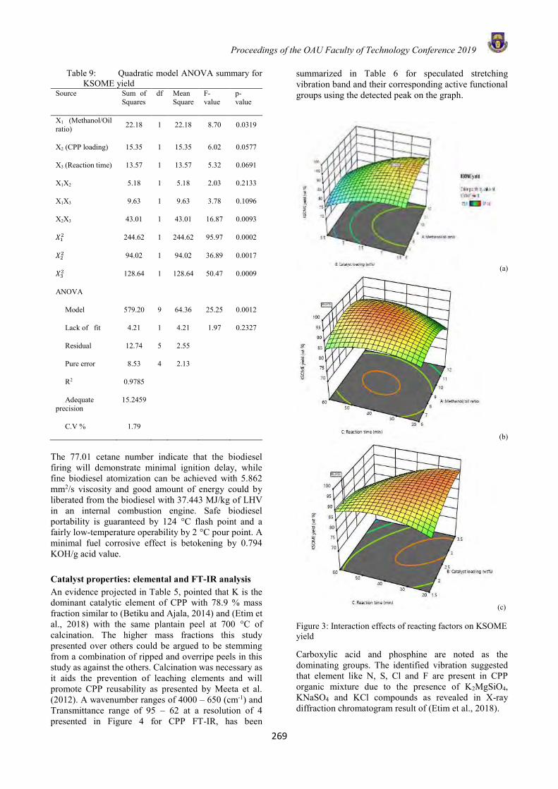
Proceedings of the OAU Faculty of Technology Conference 2019
269
Table 9: Quadratic model ANOVA summary for KSOME yield
Source Sum of Squares
df Mean Square
F-value
p-value
X1 (Methanol/Oil ratio) 22.18 1 22.18 8.70 0.0319
X2 (CPP loading) 15.35 1 15.35 6.02 0.0577
X3 (Reaction time) 13.57 1 13.57 5.32 0.0691
X1X2 5.18 1 5.18 2.03 0.2133
X1X3 9.63 1 9.63 3.78 0.1096
X2X3 43.01 1 43.01 16.87 0.0093
𝑋12 244.62 1 244.62 95.97 0.0002
𝑋22 94.02 1 94.02 36.89 0.0017
𝑋32 128.64 1 128.64 50.47 0.0009
ANOVA
Model 579.20 9 64.36 25.25 0.0012
Lack of fit 4.21 1 4.21 1.97 0.2327
Residual 12.74 5 2.55
Pure error 8.53 4 2.13
R2 0.9785
Adequate precision
15.2459
C.V % 1.79
The 77.01 cetane number indicate that the biodiesel firing will demonstrate minimal ignition delay, while fine biodiesel atomization can be achieved with 5.862 mm2/s viscosity and good amount of energy could by liberated from the biodiesel with 37.443 MJ/kg of LHV in an internal combustion engine. Safe biodiesel portability is guaranteed by 124 °C flash point and a fairly low-temperature operability by 2 °C pour point. A minimal fuel corrosive effect is betokening by 0.794 KOH/g acid value. Catalyst properties: elemental and FT-IR analysis An evidence projected in Table 5, pointed that K is the dominant catalytic element of CPP with 78.9 % mass fraction similar to (Betiku and Ajala, 2014) and (Etim et al., 2018) with the same plantain peel at 700 °C of calcination. The higher mass fractions this study presented over others could be argued to be stemming from a combination of ripped and overripe peels in this study as against the others. Calcination was necessary as it aids the prevention of leaching elements and will promote CPP reusability as presented by Meeta et al. (2012). A wavenumber ranges of 4000 – 650 (cm-1) and Transmittance range of 95 – 62 at a resolution of 4 presented in Figure 4 for CPP FT-IR, has been
summarized in Table 6 for speculated stretching vibration band and their corresponding active functional groups using the detected peak on the graph.
(a)
(b)
(c)
Figure 3: Interaction effects of reacting factors on KSOME yield
Carboxylic acid and phosphine are noted as the dominating groups. The identified vibration suggested that element like N, S, Cl and F are present in CPP organic mixture due to the presence of K2MgSiO4, KNaSO4 and KCl compounds as revealed in X-ray diffraction chromatogram result of (Etim et al., 2018).
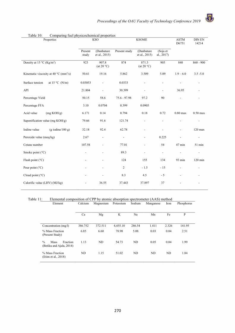
Proceedings of the OAU Faculty of Technology Conference 2019
270
Table 10: Comparing fuel physicochemical properties
Properties KSO KSOME ASTM D6751
DIN EN 14214
Present study
(Danbature et al., 2015)
Present study (Danbature et al., 2015)
(Soja et al., 2017)
Density at 15 °C (Kg/m2) 923 907.8 (at 20 °C)
874 871.3 (at 20 °C)
905 840 860 - 900
Kinematic viscosity at 40 °C (mm2/s) 50.61 19.16 5.862 3.509 5.09 1.9 – 6.0 3.5 -5.0
Surface tension at 15 °C (N/m) 0.03053 - 0.0333 - - - -
API 21.804 - 30.399 - - 36.95 -
Percentage Yield 50.15 58.6 75.6 - 97.98 97.2 90 - -
Percentage FFA 3.10 0.0704 0.399 0.0905
Acid value (mg KOH/g) 6.171 0.14 0.794 0.18 0.72 0.80 max 0.50 max
Saponification value (mg KOH/g) 79.66 91.6 121.74 - - - -
Iodine value (g iodine/100 g) 32.18 92.4 62.78 - - - 120 max
Peroxide value (meq/kg) 2.67 - - - 0.225 - -
Cetane number 107.58 - 77.01 - 54 47 min 51 min
Smoke point (°C) - - 89.3 - - - -
Flash point (°C) - - 124 155 134 93 min 120 min
Pour point (°C) - - 2 - 1.5 - 15 - -
Cloud point (°C) - - 8.3 4.5 - 5 - -
Calorific value (LHV) (MJ/kg) - 36.55 37.443 37.897 37 - -
Table 11: Elemental composition of CPP by atomic absorption spectrometer (AAS) method
Element Calcium Magnesium Potassium Sodium Manganese Iron Phosphorus
Ca Mg K Na Mn Fe P
Concentration (mg/l) 386.752 372.511 4,455.10 286.54 1.411 2.326 141.95
% Mass Fraction (Present Study)
6.85 6.60 78.90 5.08 0.03 0.04 2.51
% Mass Fraction (Betiku and Ajala, 2014)
1.13 ND 54.73 ND 0.05 0.04 1.99
% Mass Fraction (Etim et al., 2018)
ND 1.15 51.02 ND ND ND 1.84
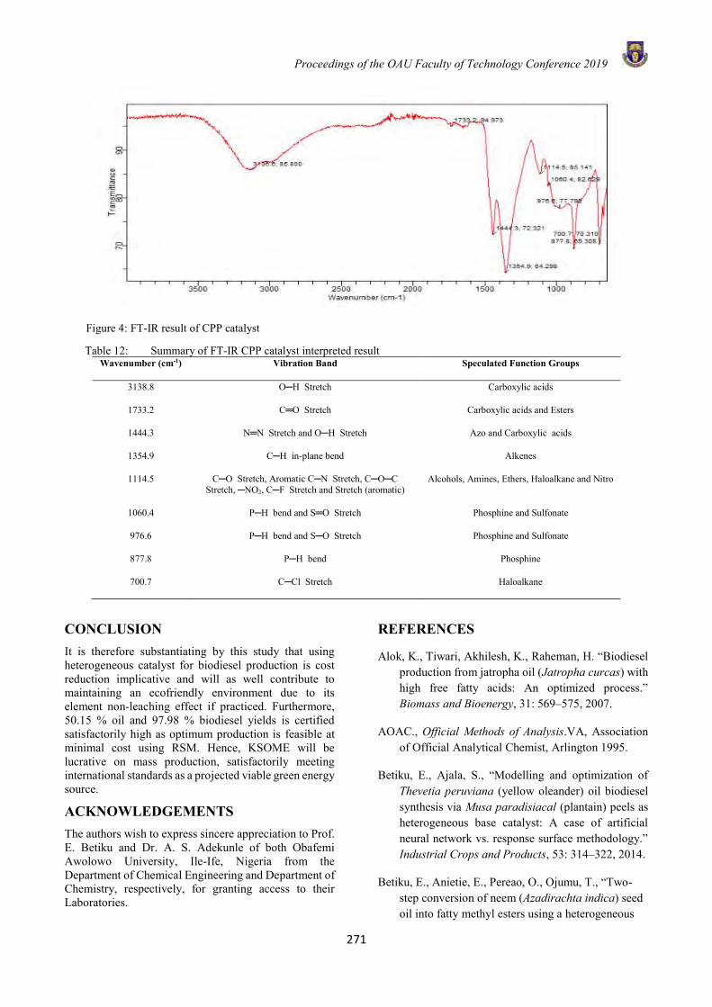
Proceedings of the OAU Faculty of Technology Conference 2019
271
Figure 4: FT-IR result of CPP catalyst
Table 12: Summary of FT-IR CPP catalyst interpreted result Wavenumber (cm-1) Vibration Band Speculated Function Groups
3138.8 OH Stretch Carboxylic acids
1733.2 CO Stretch Carboxylic acids and Esters
1444.3 NN Stretch and OH Stretch Azo and Carboxylic acids
1354.9 CH in-plane bend Alkenes
1114.5 CO Stretch, Aromatic CN Stretch, COC Stretch, NO2, CF Stretch and Stretch (aromatic)
Alcohols, Amines, Ethers, Haloalkane and Nitro
1060.4 PH bend and SO Stretch Phosphine and Sulfonate
976.6 PH bend and SO Stretch Phosphine and Sulfonate
877.8 PH bend Phosphine
700.7 CCl Stretch Haloalkane
CONCLUSION It is therefore substantiating by this study that using heterogeneous catalyst for biodiesel production is cost reduction implicative and will as well contribute to maintaining an ecofriendly environment due to its element non-leaching effect if practiced. Furthermore, 50.15 % oil and 97.98 % biodiesel yields is certified satisfactorily high as optimum production is feasible at minimal cost using RSM. Hence, KSOME will be lucrative on mass production, satisfactorily meeting international standards as a projected viable green energy source.
ACKNOWLEDGEMENTS The authors wish to express sincere appreciation to Prof. E. Betiku and Dr. A. S. Adekunle of both Obafemi Awolowo University, Ile-Ife, Nigeria from the Department of Chemical Engineering and Department of Chemistry, respectively, for granting access to their Laboratories.
REFERENCES
Alok, K., Tiwari, Akhilesh, K., Raheman, H. “Biodiesel production from jatropha oil (Jatropha curcas) with high free fatty acids: An optimized process.” Biomass and Bioenergy, 31: 569–575, 2007.
AOAC., Official Methods of Analysis.VA, Association of Official Analytical Chemist, Arlington 1995.
Betiku, E., Ajala, S., “Modelling and optimization of Thevetia peruviana (yellow oleander) oil biodiesel synthesis via Musa paradisiacal (plantain) peels as heterogeneous base catalyst: A case of artificial neural network vs. response surface methodology.” Industrial Crops and Products, 53: 314–322, 2014.
Betiku, E., Anietie, E., Pereao, O., Ojumu, T., “Two-step conversion of neem (Azadirachta indica) seed oil into fatty methyl esters using a heterogeneous
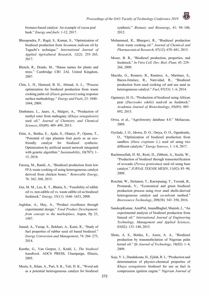
Proceedings of the OAU Faculty of Technology Conference 2019
272
biomass-based catalyst: An example of cocoa pod husk.” Energy and fuels: 1-12, 2017.
Bhoopendra, P., Ragit, S., Kumar, S., “Optimization of biodiesel production from Sesamum indicum oil by Taguchi’s technique.” International Journal of Applied Agricultural Research, 12(2): 255–265, 2017.
Blench, R., Dendo, M., “Hausa names for plants and trees.” Cambridge CB1 2AL United Kingdom, 2007.
Chin, L. H., Hameed, B. H., Ahmad, A. L., “Process optimization for biodiesel production from waste cooking palm oil (Elaeis guineensis) using response surface methodology.” Energy and Fuels, 23: 1040–1044, 2009.
Danbature, L., Jauro, A., Malgwi, A., “Production of methyl ester from mahogany (Khaya senegalensis) seed oil.” Journal of Chemistry and Chemical Sciences, 05(09): 489–499, 2015.
Etim, A., Betiku, E., Ajala, S., Olaniyi, P., Ojumu, T., “Potential of ripe plantain fruit peels as an eco-friendly catalyst for biodiesel synthesis: Optimization by artificial neural network integrated with genetic algorithm.” Sustainability, 10(707): 1–15, 2018.
Farooq, M., Ramli, A., “Biodiesel production from low FFA waste cooking oil using heterogeneous catalyst derived from chicken bones.” Renewable Energy, 76: 362–368, 2015.
Gui, M. M., Lee, K. T., Bhatia, S., “Feasibility of edible oil vs. non-edible oil vs. waste edible oil as biodiesel feedstock.” Energy, 33(11): 1646–1653, 2008.
Joglekar, A., May, A., “Product excellence through experimental design.” Food Product Development: from concept to the marketplace, Aspen, Pp 23, 1987.
Junaid, A., Yusup, S., Bokhari, A., Kami, R., “Study of fuel properties of rubber seed oil based biodiesel.” Energy Conversion and Management, 74: 266–275, 2014.
Knothe, G., Van Gerpen, J., Krahl, J., The biodiesel handbook. AOCS PRESS, Champaign, Illinois, 2005.
Meeta, S., Khan, A., Puri, S. K., Tuli, D. K., “Wood ash as a potential heterogeneous catalyst for biodiesel
synthesis.” Biomass and Bioenergy, 41: 94–106, 2012.
Mohammed, R., Bhargavi, R., “Biodiesel production from waste cooking oil.” Journal of Chemical and Pharmaceutical Research, 07(12): 670–681, 2015.
Moser, B. R., “Biodiesel production, properties, and feedstock.” In Vitro Cell. Dev. Biol.-Plant, 45: 229–266, 2009.
Muciño, G., Romero, R., Ramírez, A., Martínez, S., Baeza-Jiménez, R., Natividad, R., “Biodiesel production from used cooking oil and sea sand as heterogeneous catalyst.” Fuel, 07(53): 1–6, 2014.
Ogunsuyi, H. O., “Production of biodiesel using African pear (Dacryodes edulis) seed-oil as feedstock.” Academia Journal of Biotechnology, 03(05): 085–092, 2015.
Orwa, et al., “Agroforestry database 4.0.” Meliaceae, 2009.
Oyelade, J. O., Idowu, D. O., Oniya, O. O., Ogunkunle, O., “Optimization of biodiesel production from sandbox (Hura crepitans L.) seed oil using two different catalysts.” Energy Sources, 1: 1-8, 2017.
Rachimoellah, H. M., Resti, D., Zibbeni, A., Susila, W., “Production of biodiesel through transesterification of avocado (Persea gratissima) seed oil using base catalyst.” JURNAL TEKNIK MESIN, 11(02): 85–90, 2009.
Roschat, W., Siritanon, T., Kaewpuang, T., Yoosuk, B., Promarak, V., “Economical and green biodiesel production process using river snail shells-derived heterogeneous catalyst and co-solvent method.” Bioresource Technology, 209(38): 343–350, 2016.
SandeepKumar, AmitPal, AnandBaghel, Manish, J., “An experimental analysis of biodiesel production from linseed oil.” International Journal of Engineering Technology, Management and Applied Sciences, 03(02): 133–140, 2015.
Shote, A. S., Betiku, E., Asere, A. A., “Biodiesel production by transmethylation of Nigerian palm kernel oil.” Ife Journal of Technology, 18(02): 1–4, 2009.
Soja, Y. J., Dandakouta, H., Ejilah, R. I., “Production and determination of physico-chemical properties of Khaya senegalensis biodiesel for use as fuel in compression ignition engine.” Nigerian Journal of

Proceedings of the OAU Faculty of Technology Conference 2019
273
Engineering Science and Technology Research, 03(01): 94–103, 2017.
Van Gerpen, J., Shanks, B., Pruszko, R., Clements, D., Knothe, G. Biodiesel production technology. Subcontractor, National Renewable Energy Laboratory, Cole Boulevard, Golden, Colorado, Pp 1–110, 2004.
Vicente, G., Mart, M., “Integrated biodiesel production: A comparison of different homogeneous catalysts systems.” Bioresource Technology, 92: 297–305, 2004.
Vivek, Gupta, A. K., “Biodiesel production from karanja oil.” Journal of Scientific and Industrial Research, 63(03): 39–47, 2004.
Ying-Zhi, H., Hong, L., Wang, X.-Q., Liu, J.-Z., Jiao, J., Luo, M., Fu, Y.-J., “Biodiesel production from Pistacia chinensis seed oil via transesterification using recyclable magnetic cellulose-based catalyst.” Industrial Crops and Products, 89: 332–338, 2016.
Proceedings of the OAU Faculty of Technology Conference 2019
274
PROSPECTS OF COMBINED PEROXIDE OXIDATION AND AERATION TREATMENT PROCESSES IN ABATEMENT OF POLLUTION
CHARACTERISTICS IN CASSAVA PROCESSING WASTEWATER
O. A. Omotosho1,*, J. A. Osunbitan2 and G. A. Ogunwande2 1Land and Water Management Programme, Institute of Agricultural Research and Training, Obafemi Awolowo
University, Moor Plantation, Nigeria, 2Department of Agricultural and Environmental Engineering, Faculty of Technology,
Obafemi Awolowo University, Nigeria.
*Email of Corresponding Author: [email protected]
ABSTRACT The study investigated the efficacy of a treatment sequence consisting of a peroxide oxidation, aeration and adsorption-filtration at four different carbon depths in controlling pollution parameters from cassava processing wastewater. Analysis of results obtained revealed that concentration of selected physico-chemical parameters of effluent drawn from the established treatment lines were all within the Federal Environmental Protection Agency’s standards for discharge to water bodies with the exception of Total Suspended Solids (TSS). Statistical analysis of results showed that the effect of carbon depth on concentration of considered parameters was not significant (p 0.05) for iron, manganese, calcium and zinc while all other parameters were significant. The separation of effluent parameter means done by Duncan multiple range tests also revealed that the mean of values from the four columns were not significantly (p > 0.05) different for iron, manganese, mercury, nickel, zinc and phenol ions while those for colour, nitrate, total dissolved solids and total suspended solids were all significantly different. All other considered parameters however had two or more parameters sharing mean values that were grouped as not being significantly different. The particle index comparison for the treatment process revealed that the dual filter media columns exhibited a more stable working condition when it came to turbidity removal. The study concluded that the effluent from the sand filter and 5 cm carbon depth dual media treatment process could be safely discharged to watercourse or used for irrigation purposes. Keywords: aeration, cassava, filtration, hydrogen peroxide, wastewater INTRODUCTION In cassava processing communities, huge quantity of wastewater and solid waste are generated and could constitute an environmental menace where not adequately managed. In Nigeria, high levels of cassava effluent are produced daily and indiscriminately drained onto nearby streams, rivers and agricultural lands, thereby, constituting a serious environmental hazard. Not only does the effluent result in a strong stench, it could also result in loss of aquatic life due to its toxic nature. More recently the problem of effluents from processing operation and their disposal has gained public recognition. In many areas of the world, especially the developing countries, these environmental issues are the same (Okonko et al., 2006; Shittu et al., 2007). In south western Nigeria, cassava mill is one of the major industries and the mills are on many occasions sited in areas where the effluent is capable of causing pollution on arable lands and fresh water sources. According to Izonfuo et al. (2013) and Ehiagbonare et al. (2009), evidence have shown that concentration of contaminants present in soil samples obtained around cassava processing sites were higher than recommended values. Pollution from cassava processing wastewater has been observed to be responsible for a number of agricultural and environmental issues which include inducement of stresses and delay in germination of plants (Nwaogu et
al., 2011), mutation of plant genes (Olorunfemi et al., 2011) etc. According to Wade et al. (2002), effluent from cassava processing has also been observed to have toxic effects on aquatic life. There is therefore the need for treatment of wastewater from agricultural processing activities before they are discharged into the water courses or open fields in order to reduce potential environmental hazards (Ewemoje et al., 2011). Water is a resource that is unique to the earth and also crucial to the existence of life on it. Many authors have argued that access to clean water is gradually dwindling due to continuous pollution of existing water bodies. Over the last century, continued population growth and industrialization have resulted in the degradation of various ecosystems on which human life relies (Chan et al., 2009). As the world population increases the availability of clean water becomes a critical issue. According to Rowell (2006) it is estimated that by the year 2025, there would be an additional 2.5 billion people on the earth that will live in a region already lacking sufficient clean water. The study therefore aims at comparing the efficiency of four treatment sequences to confirm if they could offer a viable option for recycling wastewater from cassava processing activities for use in irrigation and safe discharge to water courses.
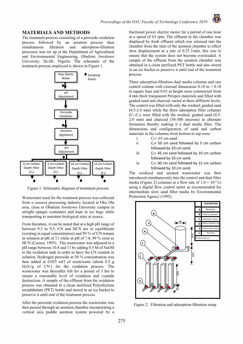
Proceedings of the OAU Faculty of Technology Conference 2019
275
MATERIALS AND METHODS The treatment process consisting of a peroxide oxidation process followed by an aeration process then simultaneous filtration and adsorption-filtration processes was set up at the Department of Agricultural and Environmental Engineering, Obafemi Awolowo University, Ile-Ife, Nigeria. The schematic of the treatment process employed is shown in Figure 1.
Figure 1: Schematic diagram of treatment process
Wastewater used for the treatment process was collected from a cassava processing industry located at Oke Ola area, close to Obafemi Awolowo University campus in airtight opaque containers and kept in ice bags while transporting to maintain biological state at source.
From literature, it can be noted that at a high pH range of between 9.3 to 9.5, CN and HCN are in equilibrium (existing in equal concentration) and 99 % of CN remain in solution at pH of 11 while at pH of 7.0, 99 % exist as HCN (Caruso, 1995). The wastewater was adjusted to a pH range between 10.8 and 11 by adding 0.5 M of NaOH to the oxidation tank in order to have the CN content in solution. Hydrogen peroxide at 50 % concentration was then added at 0.025 ml/l of wastewater (about 0.5 g H2O2/g of CN-) for the oxidation process. The wastewater was thereafter left for a period of 3 hrs to ensure a reasonable level of oxidation and cyanide destruction. A sample of the effluent from the oxidation process was obtained in a clean sterilized Polyethylene terephthalate (PET) bottle and stored in an ice bucket to preserve it until end of the treatment process. After the peroxide oxidation process the wastewater was then passed through an aeration chamber incorporating a vertical axis paddle aeration system powered by a
fractional power electric motor for a period of one hour at a speed of 65 rpm. The effluent in the chamber was displaced by fresh effluent which was released into the chamber from the inlet of the aeration chamber to effect slow displacement at a rate of 0.25 l/min, this was to ensure that the system does not become overloaded. A sample of the effluent from the aeration chamber was obtained in a clean sterilized PET bottle and also stored in an ice bucket to preserve it until end of the treatment process.
Three adsorption-filtration dual media columns and one control column with external dimensions 0.18 m × 0.18 m square base and 0.65 m height were constructed from 4 mm thick transparent Perspex materials and filled with graded sand and charcoal varied at three different levels. The control was filled with only the washed, graded sand (0.5-2.0 mm) while the three adsorption filter columns (C1-C3) were filled with the washed, graded sand (0.5-2.0 mm) and charcoal (50-300 microns) in alternate formation thereby making it a dual media filter. The dimensions and configuration of sand and carbon materials in the columns from bottom to top were:
i. C0= 65 cm sand. ii. C1= 50 cm sand followed by 5 cm carbon
followed by 10 cm sand. iii. C2= 45 cm sand followed by 10 cm carbon
followed by 10 cm sand. iv. C3= 40 cm sand followed by 15 cm carbon
followed by 10 cm sand. The oxidized and aerated wastewater was then introduced simultaneously into the control and dual filter media (Figure 2) columns at a flow rate of 1.0 × 10⁻² l/s using a digital flow control meter as recommended for intermediate slow sand filter media by Environmental Protection Agency (1995).
Figure 2: Filtration and adsorption-filtration setup
Raw Waste Water
Peroxide Oxidation
Aeration (Agitation)
pH Adjustment
Sampling Points
5 cm Carbon Depth Filter
(C1)
10 cm Carbon
Depth Filter
(C2)
15 cm Carbon
Depth Filter
(C3)
0 cm Carbon Depth Filter
(Co)
pH Adjustment
ITEM
DESCRIPTION
A Reservoir
B 140 mm diameter
PVC pipe C adsorption column
D 140mm Ø plastic tap
E 140 mm Ø air valve
F Back Nut
A
B
C
D
E
25
0
18
0
620
F
65
0
All Dimensions in
Millimeters
40
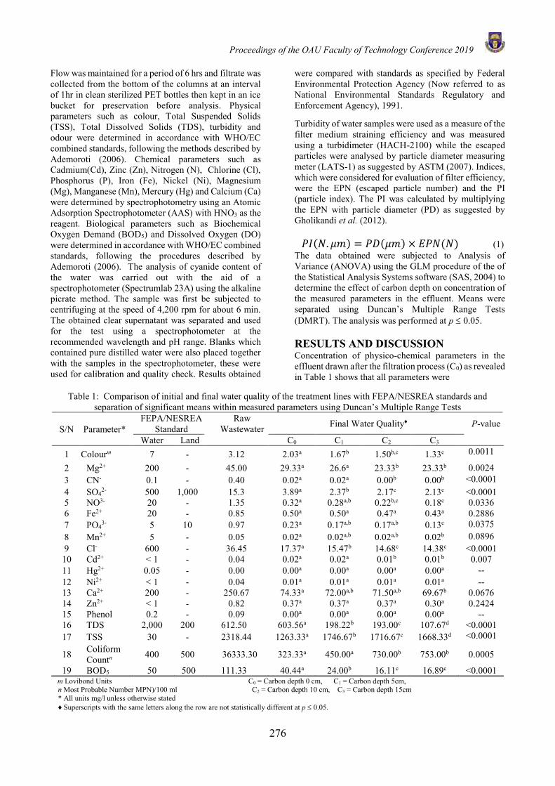
Proceedings of the OAU Faculty of Technology Conference 2019
276
Flow was maintained for a period of 6 hrs and filtrate was collected from the bottom of the columns at an interval of 1hr in clean sterilized PET bottles then kept in an ice bucket for preservation before analysis. Physical parameters such as colour, Total Suspended Solids (TSS), Total Dissolved Solids (TDS), turbidity and odour were determined in accordance with WHO/EC combined standards, following the methods described by Ademoroti (2006). Chemical parameters such as Cadmium(Cd), Zinc (Zn), Nitrogen (N), Chlorine (Cl), Phosphorus (P), Iron (Fe), Nickel (Ni), Magnesium (Mg), Manganese (Mn), Mercury (Hg) and Calcium (Ca) were determined by spectrophotometry using an Atomic Adsorption Spectrophotometer (AAS) with HNO3 as the reagent. Biological parameters such as Biochemical Oxygen Demand (BOD5) and Dissolved Oxygen (DO) were determined in accordance with WHO/EC combined standards, following the procedures described by Ademoroti (2006). The analysis of cyanide content of the water was carried out with the aid of a spectrophotometer (Spectrumlab 23A) using the alkaline picrate method. The sample was first be subjected to centrifuging at the speed of 4,200 rpm for about 6 min. The obtained clear supernatant was separated and used for the test using a spectrophotometer at the recommended wavelength and pH range. Blanks which contained pure distilled water were also placed together with the samples in the spectrophotometer, these were used for calibration and quality check. Results obtained
were compared with standards as specified by Federal Environmental Protection Agency (Now referred to as National Environmental Standards Regulatory and Enforcement Agency), 1991. Turbidity of water samples were used as a measure of the filter medium straining efficiency and was measured using a turbidimeter (HACH-2100) while the escaped particles were analysed by particle diameter measuring meter (LATS-1) as suggested by ASTM (2007). Indices, which were considered for evaluation of filter efficiency, were the EPN (escaped particle number) and the PI (particle index). The PI was calculated by multiplying the EPN with particle diameter (PD) as suggested by Gholikandi et al. (2012).
𝑃𝐼(𝑁. 𝜇𝑚) = 𝑃𝐷(𝜇𝑚) × 𝐸𝑃𝑁(𝑁) (1) The data obtained were subjected to Analysis of Variance (ANOVA) using the GLM procedure of the of the Statistical Analysis Systems software (SAS, 2004) to determine the effect of carbon depth on concentration of the measured parameters in the effluent. Means were separated using Duncan’s Multiple Range Tests (DMRT). The analysis was performed at p 0.05.
RESULTS AND DISCUSSION Concentration of physico-chemical parameters in the effluent drawn after the filtration process (C0) as revealed in Table 1 shows that all parameters were
Table 1: Comparison of initial and final water quality of the treatment lines with FEPA/NESREA standards and
separation of significant means within measured parameters using Duncan’s Multiple Range Tests
S/N Parameter* FEPA/NESREA
Standard Raw
Wastewater Final Water Quality♦ P-value
Water Land C0 C1 C2 C3 1 Colourm 7 - 3.12 2.03a 1.67b 1.50b,c 1.33c 0.0011
2 Mg2+ 200 - 45.00 29.33a 26.6a 23.33b 23.33b 0.0024 3 CN- 0.1 - 0.40 0.02a 0.02a 0.00b 0.00b <0.0001 4 SO4
2- 500 1,000 15.3 3.89a 2.37b 2.17c 2.13c <0.0001 5 NO3- 20 - 1.35 0.32a 0.28a,b 0.22b,c 0.18c 0.0336 6 Fe2+ 20 - 0.85 0.50a 0.50a 0.47a 0.43a 0.2886 7 PO4
3- 5 10 0.97 0.23a 0.17a,b 0.17a,b 0.13c 0.0375 8 Mn2+ 5 - 0.05 0.02a 0.02a,b 0.02a,b 0.02b 0.0896 9 Cl- 600 - 36.45 17.37a 15.47b 14.68c 14.38c <0.0001 10 Cd2+ < 1 - 0.04 0.02a 0.02a 0.01b 0.01b 0.007 11 Hg2+ 0.05 - 0.00 0.00a 0.00a 0.00a 0.00a -- 12 Ni2+ < 1 - 0.04 0.01a 0.01a 0.01a 0.01a -- 13 Ca2+ 200 - 250.67 74.33a 72.00a,b 71.50a,b 69.67b 0.0676 14 Zn2+ < 1 - 0.82 0.37a 0.37a 0.37a 0.30a 0.2424 15 Phenol 0.2 - 0.09 0.00a 0.00a 0.00a 0.00a -- 16 TDS 2,000 200 612.50 603.56a 198.22b 193.00c 107.67d <0.0001 17 TSS 30 - 2318.44 1263.33a 1746.67b 1716.67c 1668.33d <0.0001
18 Coliform Countn 400 500 36333.30 323.33a 450.00a 730.00b 753.00b 0.0005
19 BOD5 50 500 111.33 40.44a 24.00b 16.11c 16.89c <0.0001 m Lovibond Units C0 = Carbon depth 0 cm, C1 = Carbon depth 5cm, n Most Probable Number MPN)/100 ml C2 = Carbon depth 10 cm, C3 = Carbon depth 15cm * All units mg/l unless otherwise stated ♦ Superscripts with the same letters along the row are not statistically different at p 0.05.
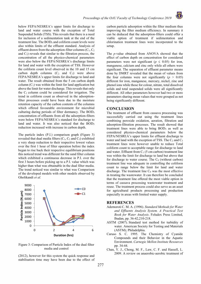
Proceedings of the OAU Faculty of Technology Conference 2019
277
below FEPA/NESREA’s upper limits for discharge to land and water course with the exception of Total Suspended Solids (TSS). This reveals that there is a need for inclusion of a sedimentation tank at the end of the treatment line. The BOD5 and coliform count levels were also within limits of the effluent standard. Analysis of effluent drawn from the adsorption-filter columns (C1, C2 and C3) reveals that similar to the filtration process, the concentration of all the physico-chemical parameters were also below the FEPA/NESREA’s discharge limits for land and water with the exception of TSS. However the coliform count level observed in the 10 and 15 cm carbon depth columns (C2 and C3) were above FEPA/NESREA’s upper limits for discharge to land and water. The result obtained from the 5 cm carbon depth column (C1) was within the limit for land application but above the limit for water discharge. This reveals that only the C1 column could be considered for irrigation. The trend in coliform count as observed in the adsorption-filter processes could have been due to the moisture retention capacity of the carbon contents of the columns which offered favourable environment for microbial culturing during periods of filter dormancy. The BOD5 concentration of effluents from all the adsorption-filters were below FEPA/NESREA’s standard for discharge to land and water. It was also noticed that the BOD5 reduction increased with increase in carbon depth.
The particle index (P.I.) comparison graph (Figure 3) revealed that dual media filters (C1, C2 and C3) exhibited a very sharp reduction to their respective lowest values over the first 1 hour of filter operation before the index began to rise back their respective equilibrium positions this noticed trend was different for the sand filter column which exhibited a continuous decrease in P.I. over the first 3 hours before picking up to a P.I. value which was higher than what was obtainable in the dual filter media. The trend noticed was similar to what was Comparison of the developed models with other models observed by Gholikandi et al.
Figure 3: Comparison of Particle Index of the dual filter media and control
(2012), however for this system the quick response and stabilisation time may have been due to the effect of
carbon particle adsorption within the filter medium thus improving the filter medium efficiency. In summary it can be deduced that the adsorption-filters could offer a viable option of treatment if sedimentation and chlorination treatment lines were incorporated to the setup. The p-value obtained from ANOVA showed that the effect of carbon depth on concentration for considered parameters were not significant (p 0.05) for iron, manganese, calcium and zinc only while all others were significant. The separation of effluent parameter means done by DMRT revealed that the mean of values from the four columns were not significantly (p > 0.05) different for iron, manganese, mercury, nickel, zinc and phenol ions while those for colour, nitrate, total dissolved solids and total suspended solids were all significantly different. All other parameters however had two or more parameters sharing mean values that were grouped as not being significantly different. CONCLUSION The treatment of effluent from cassava processing was successfully carried out using the treatment lines combining peroxide oxidation, aeration, filtration and adsorption-filtration processes. The result showed that treatment lines were able to bring BOD5 as well as considered physico-chemical parameters below the FEPA/NESREA’s upper limits for effluent discharge to water and land with the exception of TSS. The C2 and C3 treatment lines were however unable to reduce Total coliform count to acceptable range for discharge to land and water. Effluent from C1 (5 cm carbon) treatment line was within the limit for discharge to land but above that for discharge to water course. The C0 (without carbon) treatment line was adequate in controlling the coliform count to range below the limit for land and water discharge. The treatment line C0 was the most effective in treating the wastewater. It can therefore be concluded that the treatment line offered the most viable option in terms of cassava processing wastewater treatment and reuse. The treatment process could also serve as an asset for agricultural products processing and production especially in areas with limited water supply. REFERENCES Ademoroti C. M. A. (1996). Standard Methods for Water
and Effluents Analysis System. A Practical Text Book for Water Analysis. Foludex Press Limited, Ibadan, pp. 36-42,210-218.
ASTM (2007). Standard test method for turbidity of water. American Society for Testing and Materials (ASTM); Philadelphia.
Caruso S. C. 1995. The Chemistry of Cyanide Compounds and their Behavior in the Aquatic Environment. Carnegie Mellon Institute Resources pp. 34-44.
Chan, Y. J., Chong, M. F., Law, C. F. and Hassell, L. 2009. A review on anaerobic-aerobic treatment of
0
1000
2000
3000
4000
5000
6000
7000
8000
9000
0 2 4 6
Par
ticl
e I
nd
ex
(N.µ
m)
Duration (hrs)
C0
C1
Proceedings of the OAU Faculty of Technology Conference 2019
278
industrial and municipal wastewater, Chemical Engineering Journal 155, pp. 1-18.
Ehiagbonare, J. E., Adjarhore, R.Y and Enabulele, S. A. 2009. Effect of cassava effluent on Okada natural water. African Journal of Biotechnology. 8 (12) 2816-2818.
Ewemoje, T. A., Omotosho, O. A. and Abimbola, O. P. 2011. Life Cycle Assessment of hatchery production process to point-of-lay of a poultry system in a developing country. In Proceeding Nigeria Institution of Agricultural Engineers Conference (Ilorin 2010), October 2010, pp. 122–125.
FEPA 1991. National Interim Guidelines and Standards for Industrial Effluents, Gaseous Emissions and Hazardous Waste Management in Nigeria. Federal Environmental Protection Agency (Now National Environmental Standards and Regulatory Enforcement Agency).
Environmental Protection Agency (1995). Water treatment manuals on filtration. EPA, Ardcavan, Wexford, Ireland.
Gholikandi, G. B., Dehghanifard, E., Sepehr, M.N., Torabian, A., Moalej, S., Dehnavi, A., Yari, R. and Asagari, A. R. (2012) Performance Evaluation of Different Filter Media in Turbidity Removal from Water by Application of Modified Qualitative Indices. Iranian Journal of Public Health 41(4): 87–93.
Izonfuo, W., Bariweni, P. A., George, D. M. C. 2013. Soil contamination from cassava wastewater discharges in a rural community in the Niger Delta, Nigeria. Journal of Applied Science Environment Management. 17(1) 105-110.
Nwaogu, L. A., Agha, N. C., Alisi, C. S. and Ihejirika, C. E. 2011. Investigation on the effect of cassava effluent-polluted soil on germination, emergence and oxidative stress parameters of Telferia occidentalis, Journal of Biodiversity and Environmental Sciences. 1 (6), 104-111.
Okonko, I. O., Olabode, O. P., Okeleji, O. S. 2006. The role of biotechnology in the socioeconomic advancement and national development: An Overview. African Journal of Biotechnology. 5(19), 2354-2366.
Olorunfemi, D. I., Okoloko, G. E., Bakare, A. A. and Akinboro, A. 2011. Cytotoxic and Genotoxic Effects of Cassava Effluents Using Allium cepa Assay. Research Journal of Mutagenisis 1(1) 1-9.
Rowell, M. 2006. Removal of Metal ions from contaminated water using Agricultural Residues. Second International conference on Environmental compatible Forest production. Fernando passoa university, Oporto Portugal 20-22. 241-247.
SAS Institute Inc.. 2004. Statistical Analysis Software/STAT 9.1 User’s guide. Cary, NC 27513, SAS publishing, USA.
Shittu, O. B., Okonko, I. O., Akpan, I. 2007. A Comparative study on the bioremediation potentials of grounded seeds of Moringa oleifera and latex exudates of Calotropis Procera (Sodom
Apple). Nigerian Journal of Microbiology 30, 1419-1024.
Wade, J. M., Omoregie, E. and Ezenwaka 2002. Toxicity of cassava (Manihot esculanta Crantz) effluent on the Nile tilapia, Oreochromis noliticus (L) under laboratory conditions. Journal of Aquatic Science, 17, 89-94.
Proceedings of the OAU Faculty of Technology Conference 2019
279
RAPID, ACCURATE AND EFFICIENT SIMULATION AND ANALYSIS OF COMPLEX SYSTEMS USING IMN APPROXIMANTS.
O. Taiwo and T. Oladipo Dept of Chemical Engineering, Obafemi Awolowo University, Ile-Ife
[email protected] [email protected]
ABSTRACT With the availability of computer algebra systems such as Mathematica, one can now take advantage of the full power of IMN approximants to efficiently and speedily compute inverse Laplace transforms of complex functions with guaranteed accuracy, even when these defy complex analytical treatment. Nevertheless, the use of higher approximants dictates using larger number of digits in the computation in order to reduce rounding errors not only in the computation of IMN constants but also in the final evaluation of the responses. It is however clear that if the number of stipulated digits during computation is excessive, unduly large computation time will be incurred. This work gives a simple technique for determining the working precision such that the computed IMN constants have specified accuracy. It is known that functions with time delays usually suffer from limited accuracy when they are subject to numerical inversion. Consequently, this work deals with numerically inverting quasi rational distributed systems, which may have several numerator delays with a view to ensuring good accuracy. The work also gives a correlation specifying the working precision, in terms of N, which ensures that the computed IMN constant Kimax for a particular N has a stipulated accuracy. The work also reveals that the computational accuracy as well as computational speed of results of IMN approximants are favorable to those obtained using MATLAB Simulink. Keywords: IMN Approximants, Simulink, Time Delays, Laplace Inversion.
INTRODUCTION IMN approximants are a rapid technique to speedily numerically invert Laplace transforms in the general case. Taiwo and King (2002) gave an exposition of how IMN approximants could be used to efficiently and accurately invert steep, stiff and oscillatory responses which constituted difficulty to earlier investigators. Another type of functions which create some challenge to investigators in terms of accurate numerical inversion are those with time delays (Taiwo et al., 1995, Taiwo and King 2002). Consequently, this work is concerned with numerically inverting quasi rational distributed systems such as may occur in particulate systems operation such as crystallization. The transfer functions arising from such processes may have more than one delay terms in their numerators and may thus pose some challenges to accurate numerical inversion. Here, two methods have been used to evaluate their time responses, namely MATLAB Simulink and IMN approximants and the results were compared in terms of speed and accuracy. Correlations are also given of the desired working precision such that for any N, the computed Kimax for any IMN approximants of full grade would have an accuracy of at least 25.
ZAKIAN (1975) IMN APPROXIMANTS Let f(t) have a Laplace transform:
dtetfsFsfL st
−==0
)()(),( (1)
where Re(s) and f(t) is continuous for t 0 and of exponential order . The IMN approximant of f(t) is an expression of the form:
IMN(f,t) = ),(1
1
tfLKt i
N
ii
=
− (2)
Many different sets Ki , i may be defined, but for the purpose of this work, they are assumed to satisfy the relation:
= +
=N
i i
i
zK
1
z-MN e
(3)
where z
MNe− is the (M/N) Padé approximant of e-z . Let
MN = min )Re( ii . It is known that under certain conditions on f(t):
f(t) - IMN(f,t) = 0(tM+N+1) , t → 0+ (4)
whenever MN > 0. Numerical tests have been performed (Taiwo et al., 1995; Taiwo and King, 2002; Zakian and Edwards, 1978) to determine all (M,N) in
0M<N 540 for which MN > 0. Note that Mmin
denotes the minimum value of M, for a given N, for the
relationship MN > 0 to hold and such approximants are said to be of full grade.
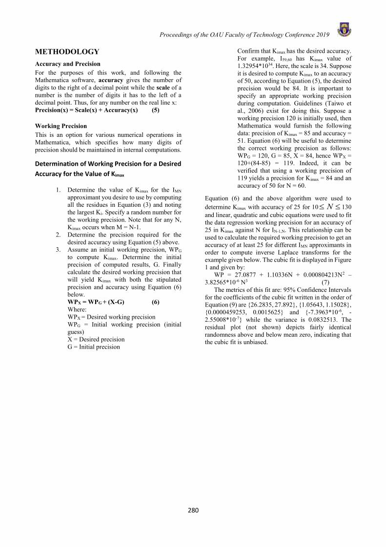
Proceedings of the OAU Faculty of Technology Conference 2019
280
METHODOLOGY Accuracy and Precision For the purposes of this work, and following the Mathematica software, accuracy gives the number of digits to the right of a decimal point while the scale of a number is the number of digits it has to the left of a decimal point. Thus, for any number on the real line x: Precision(x) = Scale(x) + Accuracy(x) (5)
Working Precision This is an option for various numerical operations in Mathematica, which specifies how many digits of precision should be maintained in internal computations. Determination of Working Precision for a Desired
Accuracy for the Value of Kimax
1. Determine the value of Kimax for the IMN approximant you desire to use by computing all the residues in Equation (3) and noting the largest Ki. Specify a random number for the working precision. Note that for any N, Kimax occurs when M = N-1.
2. Determine the precision required for the desired accuracy using Equation (5) above.
3. Assume an initial working precision, WPG to compute Kimax. Determine the initial precision of computed results, G. Finally calculate the desired working precision that will yield Kimax with both the stipulated precision and accuracy using Equation (6) below. WPX = WPG + (X-G) (6) Where: WPX = Desired working precision WPG = Initial working precision (initial guess) X = Desired precision G = Initial precision
Confirm that Kimax has the desired accuracy. For example, I59,60 has Kimax value of 1.32954*1034. Here, the scale is 34. Suppose it is desired to compute Kimax to an accuracy of 50, according to Equation (5), the desired precision would be 84. It is important to specify an appropriate working precision during computation. Guidelines (Taiwo et al., 2006) exist for doing this. Suppose a working precision 120 is initially used, then Mathematica would furnish the following data: precision of Kimax = 85 and accuracy = 51. Equation (6) will be useful to determine the correct working precision as follows: WPG = 120, G = 85, X = 84, hence WPX = 120+(84-85) = 119. Indeed, it can be verified that using a working precision of 119 yields a precision for Kimax = 84 and an accuracy of 50 for N = 60.
Equation (6) and the above algorithm were used to determine Kimax with accuracy of 25 for 10 N 130 and linear, quadratic and cubic equations were used to fit the data regression working precision for an accuracy of 25 in Kimax against N for IN-1,N. This relationship can be used to calculate the required working precision to get an accuracy of at least 25 for different IMN approximants in order to compute inverse Laplace transforms for the example given below. The cubic fit is displayed in Figure 1 and given by:
WP = 27.0877 + 1.10336N + 0.000804213N2 – 3.82565*10-6 N3 (7)
The metrics of this fit are: 95% Confidence Intervals for the coefficients of the cubic fit written in the order of Equation (9) are 26.2835, 27.892, 1.05643, 1.15028, 0.0000459253, 0.0015625 and -7.3963*10-6, -2.55008*10-7 while the variance is 0.0832513. The residual plot (not shown) depicts fairly identical randomness above and below mean zero, indicating that the cubic fit is unbiased.
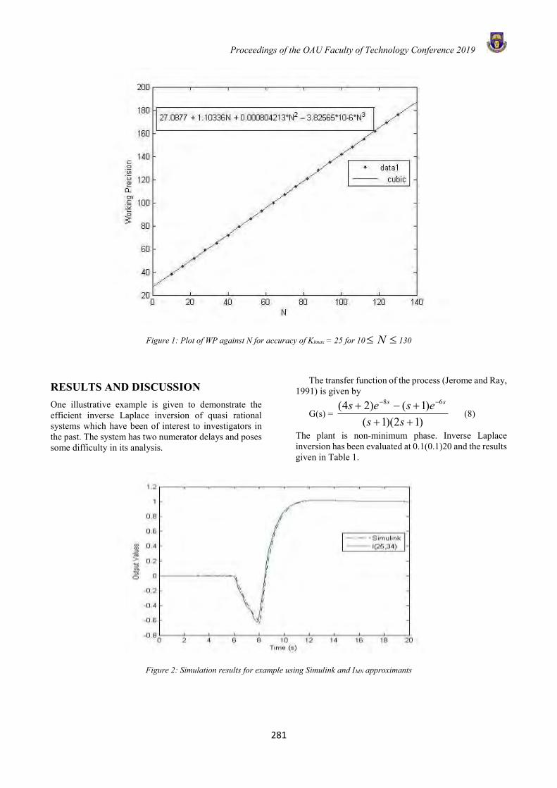
Proceedings of the OAU Faculty of Technology Conference 2019
281
Figure 1: Plot of WP against N for accuracy of Kimax = 25 for 10 N 130
RESULTS AND DISCUSSION One illustrative example is given to demonstrate the efficient inverse Laplace inversion of quasi rational systems which have been of interest to investigators in the past. The system has two numerator delays and poses some difficulty in its analysis.
The transfer function of the process (Jerome and Ray, 1991) is given by
G(s) = )12)(1(
)1()24( 68
+++−+ −−
sseses ss
(8)
The plant is non-minimum phase. Inverse Laplace inversion has been evaluated at 0.1(0.1)20 and the results given in Table 1.
Figure 2: Simulation results for example using Simulink and IMN approximants
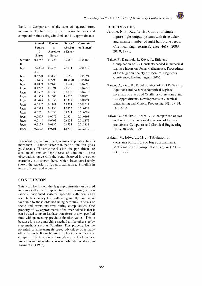
Proceedings of the OAU Faculty of Technology Conference 2019
282
Table 1: Comparison of the sum of squared error, maximum absolute error, sum of absolute error and computation time using Simulink and IMN approximants
Sum of Square
d Error
Maximum
Absolute Error
Sum of Absolute Error
Computation Time(s)
Simulink
0.1757 0.1724 2.2964 0.135186
I4,10 7.7203e-02
0.3978 7.9971 0.005372
I6,10 0.5770 0.3156 6.1659 0.005291 I9,10 1.1433 0.2296 10.9020 0.005164 I9,16 0.1839 0.2149 3.0524 0.006995 I12,16 0.1277 0.1891 2.8593 0.006950 I15,16 0.2507 0.1733 5.0026 0.006910 I14,22 0.0565 0.1505 1.4016 0.008770 I17,22 0.0445 0.1353 1.3322 0.008774 I21,22 0.0847 0.1141 2.8701 0.008611 I19,28 0.0315 0.1130 1.0973 0.010134 I23,28 0.0221 0.1030 0.9241 0.010688 I27,28 0.0495 0.0975 2.1524 0.010193 I25,34 0.0148 0.0903 0.6123 0.012872 I29,34 0.0128 0.0835 0.6531 0.012831 I33,34 0.0305 0.0751 1.6774 0.012470
In general, I25,34 approximant, whose computation time is more than 10.5 times faster than that of Simulink, gives good results. The error metrics for this approximant are also much smaller than those of Simulink. These observations agree with the trend observed in the other examples, not shown here, which have consistently shown the superiority IMN approximants to Simulink in terms of speed and accuracy.
CONCLUSION This work has shown that IMN approximants can be used to numerically invert Laplace transforms arising in quasi rational distributed systems speedily with practically acceptable accuracy. Its results are generally much more favorable to those obtained using Simulink in terms of speed and errors incurred during computations. One property of IMN approximants often overlooked is that it can be used to invert Laplace transforms at any specified time without needing previous function values. This is because it is not a marching method unlike other step by step methods such as Simulink. This property has the potential of increasing its speed advantage over many other methods. It can be used to check the accuracy of computed results whenever analytical results of Laplace inversion are not available as was earlier demonstrated in Taiwo et al. (1995).
REFERENCES Jerome, N. F., Ray, W. H., Control of single-
input/single-output systems with time delays and infinite number of right-half plane zeros. Chemical Engineering Science, 46(8): 2003–2018, 1991.
Taiwo, F., Daramola, I., Koya, N., Efficient Computation of IMN Constants needed in numerical Laplace Inversion Using Mathematica. Proceedings of the Nigerian Society of Chemical Engineers' Conference, Ibadan, Nigeria, 2006.
Taiwo, O., King, R., Rapid Solution of Stiff Differential Equations and Accurate Numerical Laplace Inversion of Steep and Oscillatory Functions using IMN Approximants. Developments in Chemical Engineering and Mineral Processing, 10(1-2): 143–164, 2002.
Taiwo, O., Schultz, J., Krebs, V., A comparison of two methods for the numerical inversion of Laplace transforms. Computers and Chemical Engineering, 19(3), 303–308, 1995.
Zakian, V., Edwards, M. J., Tabulation of constants for full grade IMN approximants. Mathematics of Computation, 32(142): 519–531, 1978.
Proceedings of the OAU Faculty of Technology Conference 2019
283
SYNTHESIS AND MICROSTRUCTURAL ANALYSIS OF FUNCTIONALLY GRADED CU-TI-NI AND ALN COMPOSITE FOR ELECTRICAL
APPLICATIONS 1,2Oyatogun A. O., 2Popoola, A. P. I., 3Popoola, O. M., 2,4Ajenifuja, E. A. 2,5Aramide, F. O.
1Oyatogun, G. M. 1Department of Materials Science and Engineering, Obafemi Awolowo University, Ile-Ife, Nigeria
2Department of Chemical, Metallurgical and Materials Engineering, Faculty of Engineering and the Built Environment, Tshwane University of Technology, Pretoria, South Africa
3Department of Electrical Engineering, Faculty of Engineering and the Built Environment, Tshwane University of Technology, Pretoria, South Africa
4 Centre for Energy Research and Development, Obafemi Awolowo University, Ile-Ife, Nigeria 5Department of Metallurgical and Materials Engineering, Federal University of Technology, Akure, Nigeria
*Email of Corresponding Author: [email protected]
ABSTRACT
Applications of copper in electronic applications have been well documented but limited by its poor mechanical properties. The development of Copper-based alloys and composites with enhanced mechanical properties is therefore vital, hence this study focused on the synthesis and microstructural analysis of functionally graded copper-based composite for electrical Applications. The incorporation of Copper (Cu) with titanium (Ti), nickel (Ni) and aluminium nitride (AlN) was applied in the synthesis of functionally graded Cu-Ti-Ni and AlN composites using spark plasma sintering techniques. The sintering conditions are 7000C – 9000C, 50 MPa, 10 minutes holding time and heating rate of 1000C/ min. Consequently, the sintered samples were taken for density measurement using Archimedes’ principles. Thereafter the samples were subjected to SEM and Energy Dispersive X-ray Spectroscopy (EDS) analysis. Micro hardness analysis was carried out on the functionally graded materials at an interval of 2.5 mm apart. Results obtained show the variation in composition of the composite across the gradient of the developed composite. These analyses revealed variation in microstructure and consequently variation in micro hardness property across this gradient. This work therefore facilitates the development of a high strength, high thermal stress resistance copper-based material to replace the toxic Cu-Be system in electrical devices for high temperature conducting applications.
Keywords: Copper, Functionally graded material, Composites, Electrical devices
INTRODUCTION Copper has been acclaimed as one of the most widely used and promising metal in electrical and manufacturing industries (Zhang et al., 2013, Sasahara, 2008, Tyler, 1990, Crane and Winter, 1986). Its use at operating temperatures greater than 100°C may however not be feasible due to its poor thermo-mechanical properties (Molina et al., 2015). Extensive research activities focused on the development of high temperature conducting copper-based materials with enhanced thermo-mechanical properties, high thermal conductivity, high electrical conductivity and ease of manufacture have been articulately documented (Liu et al., 2015, Man et al., 2014a, Sobhani et al., 2013, Vajpai et al., 2013, Kumar and Lagoudas, 2008). Alloying of copper has been established to result in improved mechanical properties of copper (Molina et al., 2015, Caron, 2001, Tyler, 1990, Crane and Winter, 1986). Alloying of copper with solutes such as titanium (Ti), nickel (Ni) and Beryllium (Be) has facilitated the development of high temperature, conducting, copper-based alloys with enhanced thermo-mechanical properties, thermal conductivity, electrical conductivity and ease of manufacture (Liu et al., 2015,
Man et al., 2014a, Sobhani et al., 2013, Vajpai et al., 2013, Xie et al., 2012, Lebreton et al., 2009, Kumar and Lagoudas, 2008, Markandeya et al., 2006, Soffa and Laughlin, 2004). Copper-beryllium (Cu-Be) alloys had been reported to have the highest thermo-mechanical properties of all the copper alloys (Li et al., 2009, Konno et al., 2008, Lu et al., 2006, Caron 2001). Its use is however limited by the environmental hazards associated with the Be–based metallurgy, which necessitated the need to replace the Cu-Be system with alternative copper-based alloy (Liu et al., 2015, Xie et al., 2012). Hence the current research drive to develop beryllium free, copper based, high strength materials with properties similar to the Cu-Be system (Liu et al., 2015, Xie et al., 2012, Soffa et al., 2004).
Copper-titanium (Cu-Ti) systems with ultra-high strength have been thoroughly researched as possible alternative to the Cu-Be system. (Liu et al., 2015, Man et al., 2014b, Sobhani et al., 2013, Lebreton et al., 2009). It was however, reported that although increasing the titanium content enhanced the strength of copper it also resulted in impaired electrical conductivity. Consequently,
Proceedings of the OAU Faculty of Technology Conference 2019
284
improving the electrical conductivity of binary Cu–Ti alloys by the ternary additions of solutes such as nickel, chromium, cadmium and aluminium to the system has been investigated (Liu et al., 2015, Man et al., 2014b, Konno et al., 2008, Markandeya et al., 2007, Markandeya et al., 2004, Nagarjuna et al., 1997). Of these solutes, the addition of nickel (Ni) to Cu-Ti binary system had been reported to results in the formation of Ni3Ti intermetallic compound that decreases the solubility of Ti in the Cu matrix while simultaneously reducing electron scattering and consequently resulting in improved electrical conductivity (Liu, et al., 2015). The decrease in titanium solubility in the copper matrix will however result in corresponding decrease in strength of the alloy, hence the need to enhance both the strength and electrical conductivity of the ternary alloy. This work therefore attempted to reinforce the Cu-Ti-Ni ternary alloy by the addition of a fourth phase, aluminium nitride, that have been reported to have high thermal conductivity, good dielectric properties, high flexural strength and high thermal expansion coefficient (Florea, 2017) to produce a high strength electrical conducting material. Functionally Graded Materials
The result of scientific progress in materials science and engineering and the continuing developments of modern industry, have given rise to the continual demand for advanced materials that can satisfy the necessary advanced properties and improved material qualities. This requirement for advanced materials with improved specific properties has brought about the gradual transformation of materials from their basic monolithic states to new level of composites. The need to develop materials with novel internal structures and intricate geometries that cannot be achieved by traditional manufacturing had led to the recent advancement in manufacturing that has resulted in a new class of materials called Functionally Graded Materials (FGM), Udupal et al., 2012, El-wazery and El-Desouky, 2015. These materials represent a second generation of composite materials that have been designed to achieve superior levels of performance.
FGMs are a type of composite material that are classified by their graded structure across the material. Specifically, an FGM typically consists of a composite material with a spatially varying property designed to optimize performance through the distribution of that property. It could be a gradual change in chemical properties, structure, grain size, texturization level, density and other physical properties from layer to layer (El-wazery and El-Desouky, 2015, Udupal et al., 2012). FGMs have a graded interface rather than a sharp interface between the two dissimilar materials. Using a material with a graded chemical composition, for example, minimizes the differences in that property from one material to another as no obvious change may take place in their chemical composition if the gradient is smooth enough. Consequently, if the transition is smooth, the mismatch in the property from one point in the material to another will
be limited. Furthermore, there will be no single location that is inherently or intrinsically weaker than the rest of the composite. In addition to these, FGM allows the ability to combine irreconcilable properties in the same component, which may not be obtainable with the use of monolithic materials. The need for property distributions is found in a variety of common products and applications that must have mutually exclusive requirements to provide multi-functional characteristics (El-Galy et al., 2017, Gupta et al., 2015, El-wazery and El-Desouky, 2015, Bharti et al., 2013, Udupal et al., 2012, Miyamoto et al., 1999). Typical example of this is found in the turbine blade in which the core must be tough enough to withstand heavy dynamic loading while its surface must have a high melting point to withstand the high temperatures to be encountered in service (El-Galy et al., 2017, Gupta et al., 2015). This work investigated the production of functionally graded Cu-Ti-Ni/AlN composite that allowed the combination of irreconcilable properties and facilitated the provision of multi-functional characteristics across the gradient.
Powder metallurgy (PM) is one of the most prevalent techniques used in the development of FGMs due to its wide range control of composition, microstructure and its ability to form a near net shape (Kumar and Chandrappa, 2014, Erdemir, et al., 2015). Spark plasma sintering (SPS) is one of the powder metallurgy techniques that have been successfully used to fabricate functionally graded materials for diverse engineering applications (Tokita, 2000, Tokita, 2014 Knaislová et al., 2017). It is a hybrid electrical–mechanical method used for rapid sintering of metallic and ceramic powders that is accomplished by the simultaneous delivery of heat and pressure to the powder. It entails the use of uniaxial force and a pulsed (on-off) direct electrical current (DC) under low atmospheric pressure to perform high speed consolidation of the powder. This direct heating allows the application of very high heating and cooling rates, which enhance densification over grain growth and promotes diffusion mechanisms thus maintaining the intrinsic properties of nanopowders in the fully dense products (Suarez et al., 2009, Alvarez-Clemares et al., 2010).
SPS has been reported to be environmentally friendly, less time consuming and energy saving (Bhavar et al., 2017, El-Galy et al., 2017, Knaislová, et al., 2017). Consequently, this technique was adopted in this research to develop the functionally graded Cu-Ti-Ni-/AlN composite that will allow the combination of irreconcilable properties by varying spatial composition profile.
MATERIALS AND METHODS
Very fine powders consisting of (>99%) purity of Copper (Centerline, Windsor, Canada), Nickel (Ni), Titanium (Ti), and Aluminum Nitride, (Sigma-Aldrich Laborchemickalien GMBH, Seelze, Germany), with physical properties indicated in Table 1.0., were premixed in graduated stoichiometric ratios, as indicated in Table
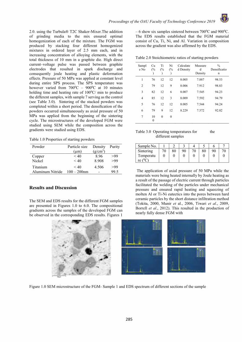
Proceedings of the OAU Faculty of Technology Conference 2019
285
2.0. using the Turbula® T2C Shaker-Mixer.The addition of grinding media to the mix ensured optimal homogenization of each of the mixture. The FGM was produced by stacking four different homogenized mixtures in ordered layer of 2.5 mm each, and in increasing concentration of alloying elements, with the total thickness of 10 mm in a graphite die. High direct current–voltage pulse was passed between graphite electrodes that resulted in spark discharge and consequently joule heating and plastic deformation effects. Pressure of 50 MPa was applied at constant level during entire SPS process. The SPS temperature was however varied from 7000C – 9000C at 10 minutes holding time and heating rate of 1000C/ min to produce the different samples, with sample 7 serving as the control (see Table 3.0). Sintering of the stacked powders was completed within a short period. The densification of the powders occurred simultaneously as axial pressure of 50 MPa was applied from the beginning of the sintering cycle. The microstructures of the developed FGM were studied using SEM while the composition across the gradients were studied using EDS.
Table 1.0 Properties of starting powders
Powder Particle size (µm)
Density (g/cm3)
Purity
Copper < 40 8.96 >99 Nickel < 40 8.908 >99 Titanium < 40 4.506 >99 Aluminum Nitride 100 – 200nm - 99.5
Results and Discussion
The SEM and EDS results for the different FGM samples are presented in Figures 1.0 to 6.0. The compositional gradients across the samples of the developed FGM can be observed in the corresponding EDS results. Figures 1
– 6 show six samples sintered between 7000C and 9000C. The EDS results established that the FGM material consist of Cu, Ti, Ni, and Al. Variation in composition across the gradient was also affirmed by the EDS.
Table 2.0 Stoichiometric ratios of starting powders
Sample No
Cu (%)
Ti (%)
Ni (%)
Calculated Density
Measured
Density
% Densificatio
n
1 76 12 12 8.005 7.887 98.53
2 79 12 9 8.006 7.912 98.83
3 82 12 6 8.007 7.545 94.23
4 85 12 3 8.009 7.592 94.79
5 76 12 12 8.005 7.544 94.24
6 79 9 12 8.229 7.572 92.02
7 100
0 0
Table 3.0 Operating temperatures for the
different samples
Sample No. 1 2 3 4 5 6 7 Sintering Temperature (0C)
700
800
900
700
800
900
700
The application of axial pressure of 50 MPa while the materials were being heated internally by Joule heating as a result of the passage of electric current through particles facilitated the welding of the particles under mechanical pressure and ensured rapid heating and squeezing of molten Al or Ti-Ni eutectics into the pores between hard ceramic particles by the short distance infiltration method (Tokita, 2000, Munir et al., 2006, Tiwari et al., 2009, Borrell et al., 2012). This resulted in the production of nearly fully dense FGM with
Figure 1.0 SEM microstructure of the FGM- Sample 1 and EDS spectrum of different sections of the sample
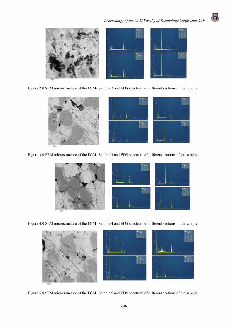
Proceedings of the OAU Faculty of Technology Conference 2019
286
Figure 2.0 SEM microstructure of the FGM- Sample 2 and EDS spectrum of different sections of the sample
Figure 3.0 SEM microstructure of the FGM- Sample 3 and EDS spectrum of different sections of the sample
Figure 4.0 SEM microstructure of the FGM- Sample 4 and EDS spectrum of different sections of the sample
Figure 5.0 SEM microstructure of the FGM- Sample 5 and EDS spectrum of different sections of the sample
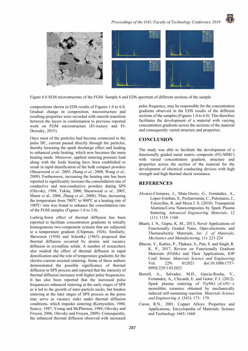
Proceedings of the OAU Faculty of Technology Conference 2019
287
Figure 6.0 SEM microstructure of the FGM- Sample 6 and EDS spectrum of different sections of the sample
compositions shown in EDS results of Figures 1.0 to 6.0. Gradual change in composition, microstructure and resulting properties were recorded with smooth transition between the layers in conformation to previous reported work on FGM microstructure (El-wazery and El-Desouky, 2015).
Once most of the particles had become connected to the pulse DC, current passed directly through the particles, thereby lessening the spark discharge effect and leading to enhanced joule heating, which now becomes the main heating mode. Moreover, applied sintering pressure load along with the Joule heating have been established to result in rapid densification of the bulk compact powders (Shearwood et al., 2005, Zhang et al., 2008, Wang et al., 2009). Furthermore, increasing the heating rate has been reported to significantly increase the consolidation rate of conductive and non-conductive powders during SPS (Olevsky, 1998, Tokita, 2000, Shearwood et al., 2005, Munir et al., 2006, Zhang et al., 2008). Thus, increasing the temperature from 7000C to 9000C at a heating rate of 1000C/ min was found to enhance the consolidation rate of the FGM samples (Figures 1.0 to 3.0).
Ludwig-Soret effect of thermal diffusion has been reported to facilitate concentration gradients in initially homogeneous two-component systems that are subjected to a temperature gradient (Chipman, 1926). Similarly, Shewmon (1958) and Schottky (1965) proposed that thermal diffusion occurred by atomic and vacancy diffusion in crystalline solids. A number of researchers also studied the effect of thermal diffusion in rapid densification and the role of temperature gradients for the electric-current assisted sintering. Some of these authors demonstrated the possible significance of thermal diffusion in SPS process and reported that the intensity of thermal diffusion increases with higher pulse frequencies. It has also been reported that the increased pulse frequencies enhanced sintering at the early stages of SPS as it led to the growth of inter-particle necks, but hinders sintering at the later stages of SPS process as the pores may serve as vacancy sinks under thermal diffusion conditions, which impedes sintering (Kornyushin, 1980, Searcy, 1987, Young and McPherson, 1989, Olevsky and Froyen, 2006, Olevsky and Froyen, 2009). Consequently, the enhanced thermal diffusion observed with increased
pulse frequency, may be responsible for the concentration gradients observed in the EDS results of the different sections of the samples (Figures 1.0 to 6.0). This therefore facilitates the development of a material with varying concentration gradients across the sections of the material and consequently varied structure and properties.
CONCLUSION
The study was able to facilitate the development of a functionally graded metal matrix composite (FG-MMC) with varied concentration gradient, structure and properties across the section of the material for the development of electrical conducting devices with high strength and high thermal shock resistance.
REFERENCES
Alvarez-Clemares, I., Mata-Osoro, G., Fernández, A., Lopez-Esteban, S., Pecharromán, C., Palomares, J., Torrecillas, R. and Moya J. S. (2010). Transparent Alumina/Ceria Nanocomposites by Spark Plasma Sintering. Advanced Engineering Materials, 12 (11): 1154–1160
Bharti, I. N., Gupta, K. M., 2013, Novel Applications of Functionally Graded Nano, Opto-electronic and Thermoelectric Materials, Int. J. of Materials, Mechanics and Manufacturing, (1): 221-224
Bhavar, V., Kattire, P., Thakare, S., Pati, S. and Singh, R. K. P., 2017, Review on Functionally Gradient Materials (FGMs) and Their Applications, IOP Conf. Series: Materials Science and Engineering Vol. 229: 012021 doi:10.1088/1757-899X/229/1/012021
Borrell, A., Salvador, M.D., García-Rocha, V., Fernández, A., Chicardi, E. and Gotor, F.J. (2012). Spark plasma sintering of TiyNb1−yCxN1−x monolithic ceramics obtained by mechanically induced self-sustaining reaction. Materials Science and Engineering A. (543): 173– 179.
Caron, R.N., 2001, Copper Alloys: Properties and Applications, Encyclopedia of Materials: Science and Technology 1665–1668
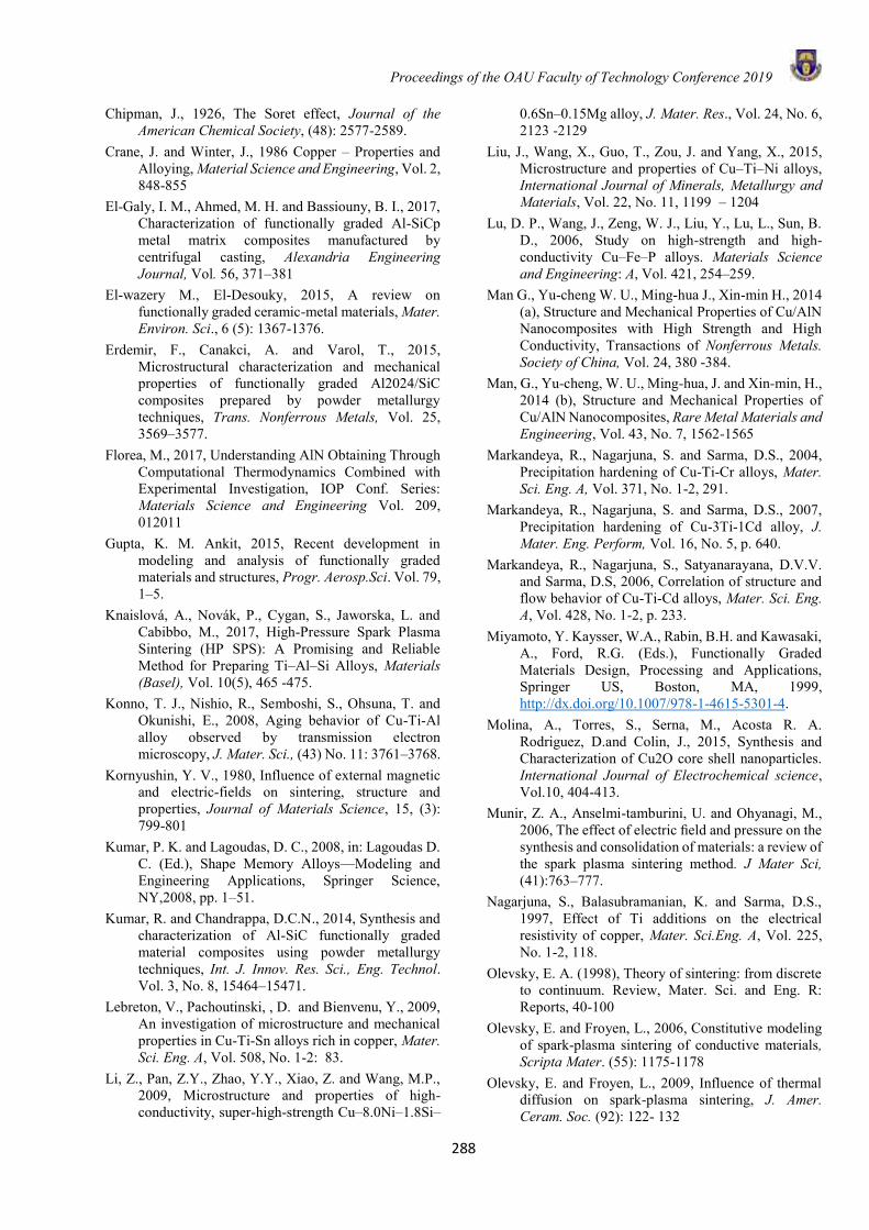
Proceedings of the OAU Faculty of Technology Conference 2019
288
Chipman, J., 1926, The Soret effect, Journal of the American Chemical Society, (48): 2577-2589.
Crane, J. and Winter, J., 1986 Copper – Properties and Alloying, Material Science and Engineering, Vol. 2, 848-855
El-Galy, I. M., Ahmed, M. H. and Bassiouny, B. I., 2017, Characterization of functionally graded Al-SiCp metal matrix composites manufactured by centrifugal casting, Alexandria Engineering Journal, Vol. 56, 371–381
El-wazery M., El-Desouky, 2015, A review on functionally graded ceramic-metal materials, Mater. Environ. Sci., 6 (5): 1367-1376.
Erdemir, F., Canakci, A. and Varol, T., 2015, Microstructural characterization and mechanical properties of functionally graded Al2024/SiC composites prepared by powder metallurgy techniques, Trans. Nonferrous Metals, Vol. 25, 3569–3577.
Florea, M., 2017, Understanding AlN Obtaining Through Computational Thermodynamics Combined with Experimental Investigation, IOP Conf. Series: Materials Science and Engineering Vol. 209, 012011
Gupta, K. M. Ankit, 2015, Recent development in modeling and analysis of functionally graded materials and structures, Progr. Aerosp.Sci. Vol. 79, 1–5.
Knaislová, A., Novák, P., Cygan, S., Jaworska, L. and Cabibbo, M., 2017, High-Pressure Spark Plasma Sintering (HP SPS): A Promising and Reliable Method for Preparing Ti–Al–Si Alloys, Materials (Basel), Vol. 10(5), 465 -475.
Konno, T. J., Nishio, R., Semboshi, S., Ohsuna, T. and Okunishi, E., 2008, Aging behavior of Cu-Ti-Al alloy observed by transmission electron microscopy, J. Mater. Sci., (43) No. 11: 3761–3768.
Kornyushin, Y. V., 1980, Influence of external magnetic and electric-fields on sintering, structure and properties, Journal of Materials Science, 15, (3): 799-801
Kumar, P. K. and Lagoudas, D. C., 2008, in: Lagoudas D. C. (Ed.), Shape Memory Alloys—Modeling and Engineering Applications, Springer Science, NY,2008, pp. 1–51.
Kumar, R. and Chandrappa, D.C.N., 2014, Synthesis and characterization of Al-SiC functionally graded material composites using powder metallurgy techniques, Int. J. Innov. Res. Sci., Eng. Technol. Vol. 3, No. 8, 15464–15471.
Lebreton, V., Pachoutinski, , D. and Bienvenu, Y., 2009, An investigation of microstructure and mechanical properties in Cu-Ti-Sn alloys rich in copper, Mater. Sci. Eng. A, Vol. 508, No. 1-2: 83.
Li, Z., Pan, Z.Y., Zhao, Y.Y., Xiao, Z. and Wang, M.P., 2009, Microstructure and properties of high-conductivity, super-high-strength Cu–8.0Ni–1.8Si–
0.6Sn–0.15Mg alloy, J. Mater. Res., Vol. 24, No. 6, 2123 -2129
Liu, J., Wang, X., Guo, T., Zou, J. and Yang, X., 2015, Microstructure and properties of Cu–Ti–Ni alloys, International Journal of Minerals, Metallurgy and Materials, Vol. 22, No. 11, 1199 – 1204
Lu, D. P., Wang, J., Zeng, W. J., Liu, Y., Lu, L., Sun, B. D., 2006, Study on high-strength and high-conductivity Cu–Fe–P alloys. Materials Science and Engineering: A, Vol. 421, 254–259.
Man G., Yu-cheng W. U., Ming-hua J., Xin-min H., 2014 (a), Structure and Mechanical Properties of Cu/AlN Nanocomposites with High Strength and High Conductivity, Transactions of Nonferrous Metals. Society of China, Vol. 24, 380 -384.
Man, G., Yu-cheng, W. U., Ming-hua, J. and Xin-min, H., 2014 (b), Structure and Mechanical Properties of Cu/AlN Nanocomposites, Rare Metal Materials and Engineering, Vol. 43, No. 7, 1562-1565
Markandeya, R., Nagarjuna, S. and Sarma, D.S., 2004, Precipitation hardening of Cu-Ti-Cr alloys, Mater. Sci. Eng. A, Vol. 371, No. 1-2, 291.
Markandeya, R., Nagarjuna, S. and Sarma, D.S., 2007, Precipitation hardening of Cu-3Ti-1Cd alloy, J. Mater. Eng. Perform, Vol. 16, No. 5, p. 640.
Markandeya, R., Nagarjuna, S., Satyanarayana, D.V.V. and Sarma, D.S, 2006, Correlation of structure and flow behavior of Cu-Ti-Cd alloys, Mater. Sci. Eng. A, Vol. 428, No. 1-2, p. 233.
Miyamoto, Y. Kaysser, W.A., Rabin, B.H. and Kawasaki, A., Ford, R.G. (Eds.), Functionally Graded Materials Design, Processing and Applications, Springer US, Boston, MA, 1999, http://dx.doi.org/10.1007/978-1-4615-5301-4.
Molina, A., Torres, S., Serna, M., Acosta R. A. Rodriguez, D.and Colin, J., 2015, Synthesis and Characterization of Cu2O core shell nanoparticles. International Journal of Electrochemical science, Vol.10, 404-413.
Munir, Z. A., Anselmi-tamburini, U. and Ohyanagi, M., 2006, The effect of electric field and pressure on the synthesis and consolidation of materials: a review of the spark plasma sintering method. J Mater Sci, (41):763–777.
Nagarjuna, S., Balasubramanian, K. and Sarma, D.S., 1997, Effect of Ti additions on the electrical resistivity of copper, Mater. Sci.Eng. A, Vol. 225, No. 1-2, 118.
Olevsky, E. A. (1998), Theory of sintering: from discrete to continuum. Review, Mater. Sci. and Eng. R: Reports, 40-100
Olevsky, E. and Froyen, L., 2006, Constitutive modeling of spark-plasma sintering of conductive materials, Scripta Mater. (55): 1175-1178
Olevsky, E. and Froyen, L., 2009, Influence of thermal diffusion on spark-plasma sintering, J. Amer. Ceram. Soc. (92): 122- 132
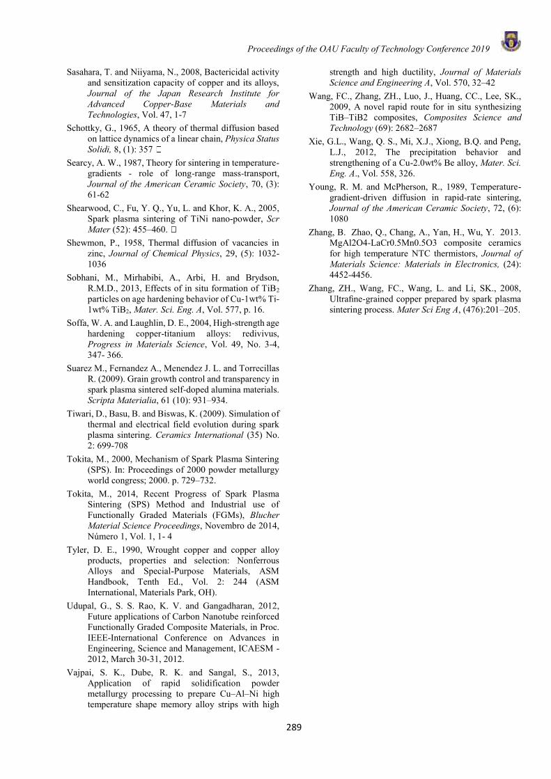
Proceedings of the OAU Faculty of Technology Conference 2019
289
Sasahara, T. and Niiyama, N., 2008, Bactericidal activity and sensitization capacity of copper and its alloys, Journal of the Japan Research Institute for Advanced Copper-Base Materials and Technologies, Vol. 47, 1-7
Schottky, G., 1965, A theory of thermal diffusion based on lattice dynamics of a linear chain, Physica Status Solidi, 8, (1): 357
Searcy, A. W., 1987, Theory for sintering in temperature-gradients - role of long-range mass-transport, Journal of the American Ceramic Society, 70, (3): 61-62
Shearwood, C., Fu, Y. Q., Yu, L. and Khor, K. A., 2005, Spark plasma sintering of TiNi nano-powder, Scr Mater (52): 455–460.
Shewmon, P., 1958, Thermal diffusion of vacancies in zinc, Journal of Chemical Physics, 29, (5): 1032-1036
Sobhani, M., Mirhabibi, A., Arbi, H. and Brydson, R.M.D., 2013, Effects of in situ formation of TiB2 particles on age hardening behavior of Cu-1wt% Ti-1wt% TiB2, Mater. Sci. Eng. A, Vol. 577, p. 16.
Soffa, W. A. and Laughlin, D. E., 2004, High-strength age hardening copper-titanium alloys: redivivus, Progress in Materials Science, Vol. 49, No. 3-4, 347- 366.
Suarez M., Fernandez A., Menendez J. L. and Torrecillas R. (2009). Grain growth control and transparency in spark plasma sintered self-doped alumina materials. Scripta Materialia, 61 (10): 931–934.
Tiwari, D., Basu, B. and Biswas, K. (2009). Simulation of thermal and electrical field evolution during spark plasma sintering. Ceramics International (35) No. 2: 699-708
Tokita, M., 2000, Mechanism of Spark Plasma Sintering (SPS). In: Proceedings of 2000 powder metallurgy world congress; 2000. p. 729–732.
Tokita, M., 2014, Recent Progress of Spark Plasma Sintering (SPS) Method and Industrial use of Functionally Graded Materials (FGMs), Blucher Material Science Proceedings, Novembro de 2014, Número 1, Vol. 1, 1- 4
Tyler, D. E., 1990, Wrought copper and copper alloy products, properties and selection: Nonferrous Alloys and Special-Purpose Materials, ASM Handbook, Tenth Ed., Vol. 2: 244 (ASM International, Materials Park, OH).
Udupal, G., S. S. Rao, K. V. and Gangadharan, 2012, Future applications of Carbon Nanotube reinforced Functionally Graded Composite Materials, in Proc. IEEE-International Conference on Advances in Engineering, Science and Management, ICAESM -2012, March 30-31, 2012.
Vajpai, S. K., Dube, R. K. and Sangal, S., 2013, Application of rapid solidification powder metallurgy processing to prepare Cu–Al–Ni high temperature shape memory alloy strips with high
strength and high ductility, Journal of Materials Science and Engineering A, Vol. 570, 32–42
Wang, FC., Zhang, ZH., Luo, J., Huang, CC., Lee, SK., 2009, A novel rapid route for in situ synthesizing TiB–TiB2 composites, Composites Science and Technology (69): 2682–2687
Xie, G.L., Wang, Q. S., Mi, X.J., Xiong, B.Q. and Peng, L.J., 2012, The precipitation behavior and strengthening of a Cu-2.0wt% Be alloy, Mater. Sci. Eng. A., Vol. 558, 326.
Young, R. M. and McPherson, R., 1989, Temperature-gradient-driven diffusion in rapid-rate sintering, Journal of the American Ceramic Society, 72, (6): 1080
Zhang, B. Zhao, Q., Chang, A., Yan, H., Wu, Y. 2013. MgAl2O4-LaCr0.5Mn0.5O3 composite ceramics for high temperature NTC thermistors, Journal of Materials Science: Materials in Electronics, (24): 4452-4456.
Zhang, ZH., Wang, FC., Wang, L. and Li, SK., 2008, Ultrafine-grained copper prepared by spark plasma sintering process. Mater Sci Eng A, (476):201–205.
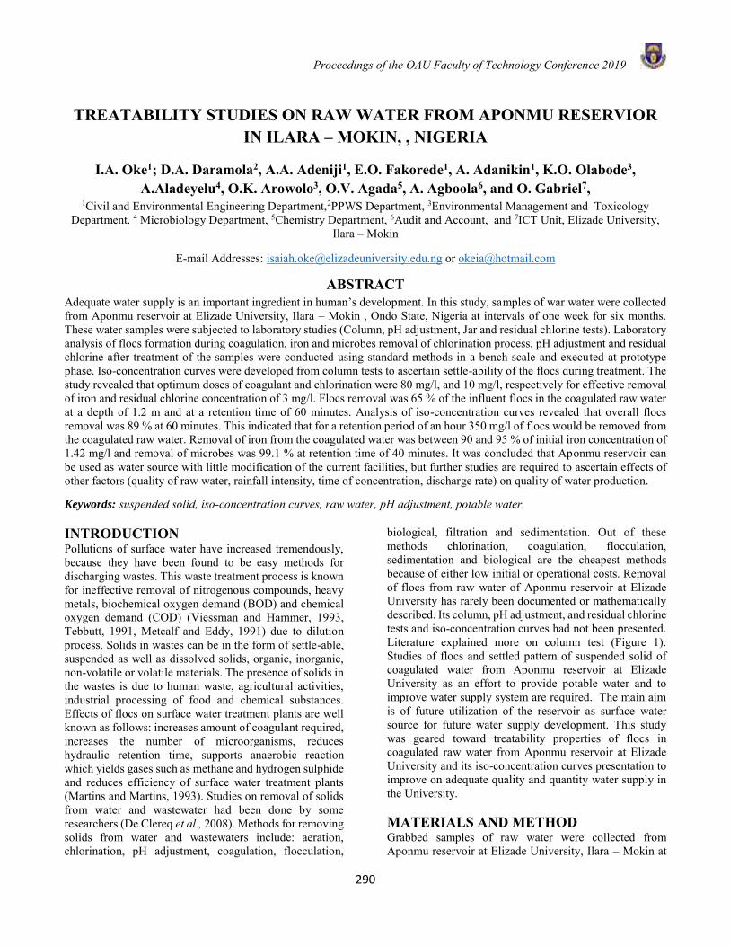
Proceedings of the OAU Faculty of Technology Conference 2019
290
TREATABILITY STUDIES ON RAW WATER FROM APONMU RESERVIOR IN ILARA – MOKIN, , NIGERIA
I.A. Oke1; D.A. Daramola2, A.A. Adeniji1, E.O. Fakorede1, A. Adanikin1, K.O. Olabode3, A.Aladeyelu4, O.K. Arowolo3, O.V. Agada5, A. Agboola6, and O. Gabriel7,
1Civil and Environmental Engineering Department,2PPWS Department, 3Environmental Management and Toxicology Department. 4 Microbiology Department, 5Chemistry Department, 6Audit and Account, and 7ICT Unit, Elizade University,
Ilara – Mokin
E-mail Addresses: [email protected] or [email protected]
ABSTRACT Adequate water supply is an important ingredient in human’s development. In this study, samples of war water were collected from Aponmu reservoir at Elizade University, Ilara – Mokin , Ondo State, Nigeria at intervals of one week for six months. These water samples were subjected to laboratory studies (Column, pH adjustment, Jar and residual chlorine tests). Laboratory analysis of flocs formation during coagulation, iron and microbes removal of chlorination process, pH adjustment and residual chlorine after treatment of the samples were conducted using standard methods in a bench scale and executed at prototype phase. Iso-concentration curves were developed from column tests to ascertain settle-ability of the flocs during treatment. The study revealed that optimum doses of coagulant and chlorination were 80 mg/l, and 10 mg/l, respectively for effective removal of iron and residual chlorine concentration of 3 mg/l. Flocs removal was 65 % of the influent flocs in the coagulated raw water at a depth of 1.2 m and at a retention time of 60 minutes. Analysis of iso-concentration curves revealed that overall flocs removal was 89 % at 60 minutes. This indicated that for a retention period of an hour 350 mg/l of flocs would be removed from the coagulated raw water. Removal of iron from the coagulated water was between 90 and 95 % of initial iron concentration of 1.42 mg/l and removal of microbes was 99.1 % at retention time of 40 minutes. It was concluded that Aponmu reservoir can be used as water source with little modification of the current facilities, but further studies are required to ascertain effects of other factors (quality of raw water, rainfall intensity, time of concentration, discharge rate) on quality of water production. Keywords: suspended solid, iso-concentration curves, raw water, pH adjustment, potable water.
INTRODUCTION Pollutions of surface water have increased tremendously, because they have been found to be easy methods for discharging wastes. This waste treatment process is known for ineffective removal of nitrogenous compounds, heavy metals, biochemical oxygen demand (BOD) and chemical oxygen demand (COD) (Viessman and Hammer, 1993, Tebbutt, 1991, Metcalf and Eddy, 1991) due to dilution process. Solids in wastes can be in the form of settle-able, suspended as well as dissolved solids, organic, inorganic, non-volatile or volatile materials. The presence of solids in the wastes is due to human waste, agricultural activities, industrial processing of food and chemical substances. Effects of flocs on surface water treatment plants are well known as follows: increases amount of coagulant required, increases the number of microorganisms, reduces hydraulic retention time, supports anaerobic reaction which yields gases such as methane and hydrogen sulphide and reduces efficiency of surface water treatment plants (Martins and Martins, 1993). Studies on removal of solids from water and wastewater had been done by some researchers (De Clereq et al., 2008). Methods for removing solids from water and wastewaters include: aeration, chlorination, pH adjustment, coagulation, flocculation,
biological, filtration and sedimentation. Out of these methods chlorination, coagulation, flocculation, sedimentation and biological are the cheapest methods because of either low initial or operational costs. Removal of flocs from raw water of Aponmu reservoir at Elizade University has rarely been documented or mathematically described. Its column, pH adjustment, and residual chlorine tests and iso-concentration curves had not been presented. Literature explained more on column test (Figure 1). Studies of flocs and settled pattern of suspended solid of coagulated water from Aponmu reservoir at Elizade University as an effort to provide potable water and to improve water supply system are required. The main aim is of future utilization of the reservoir as surface water source for future water supply development. This study was geared toward treatability properties of flocs in coagulated raw water from Aponmu reservoir at Elizade University and its iso-concentration curves presentation to improve on adequate quality and quantity water supply in the University. MATERIALS AND METHOD Grabbed samples of raw water were collected from Aponmu reservoir at Elizade University, Ilara – Mokin at
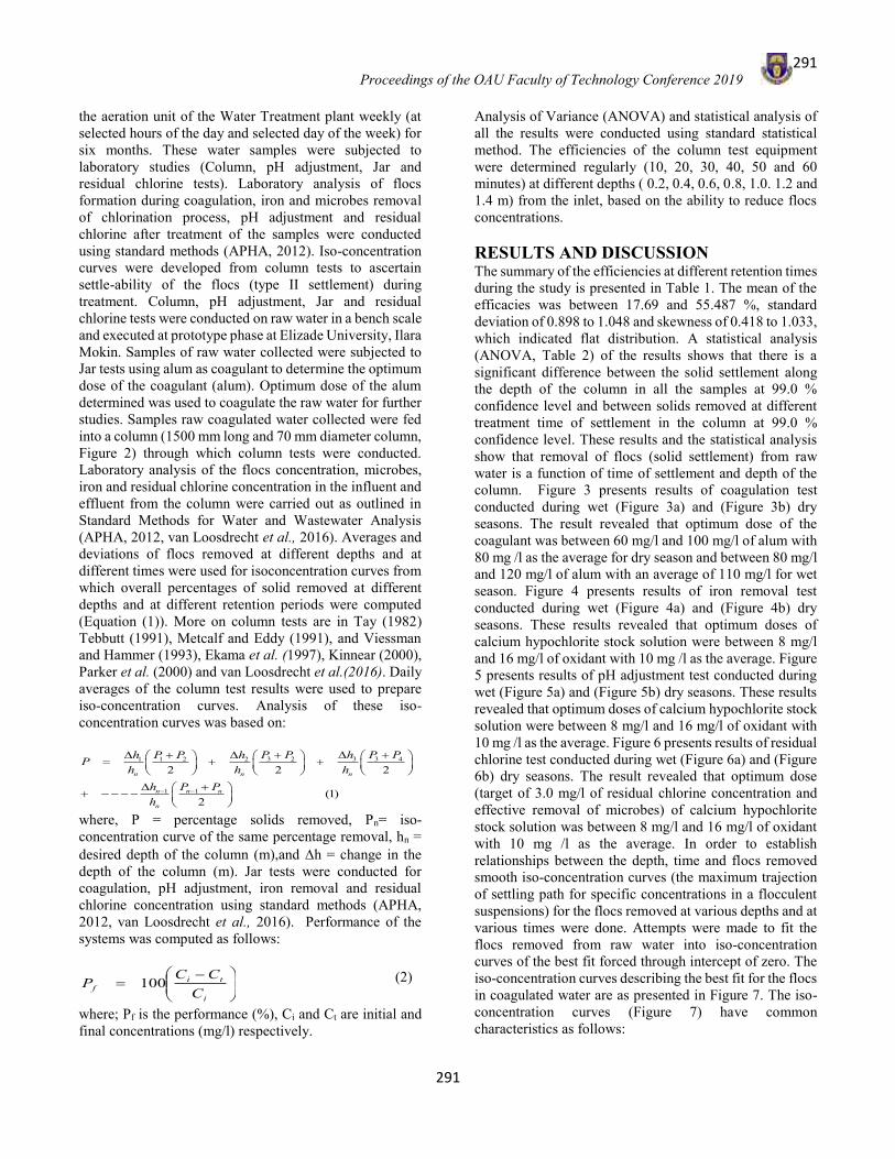
Proceedings of the OAU Faculty of Technology Conference 2019
291
291
the aeration unit of the Water Treatment plant weekly (at selected hours of the day and selected day of the week) for six months. These water samples were subjected to laboratory studies (Column, pH adjustment, Jar and residual chlorine tests). Laboratory analysis of flocs formation during coagulation, iron and microbes removal of chlorination process, pH adjustment and residual chlorine after treatment of the samples were conducted using standard methods (APHA, 2012). Iso-concentration curves were developed from column tests to ascertain settle-ability of the flocs (type II settlement) during treatment. Column, pH adjustment, Jar and residual chlorine tests were conducted on raw water in a bench scale and executed at prototype phase at Elizade University, Ilara Mokin. Samples of raw water collected were subjected to Jar tests using alum as coagulant to determine the optimum dose of the coagulant (alum). Optimum dose of the alum determined was used to coagulate the raw water for further studies. Samples raw coagulated water collected were fed into a column (1500 mm long and 70 mm diameter column, Figure 2) through which column tests were conducted. Laboratory analysis of the flocs concentration, microbes, iron and residual chlorine concentration in the influent and effluent from the column were carried out as outlined in Standard Methods for Water and Wastewater Analysis (APHA, 2012, van Loosdrecht et al., 2016). Averages and deviations of flocs removed at different depths and at different times were used for isoconcentration curves from which overall percentages of solid removed at different depths and at different retention periods were computed (Equation (1)). More on column tests are in Tay (1982) Tebbutt (1991), Metcalf and Eddy (1991), and Viessman and Hammer (1993), Ekama et al. (1997), Kinnear (2000), Parker et al. (2000) and van Loosdrecht et al.(2016). Daily averages of the column test results were used to prepare iso-concentration curves. Analysis of these iso-concentration curves was based on:
3 2 3 3 41 1 2 2
1 1
2 2 2
(1)2
n n n
n n n
n
P P h P Ph P P hPh h h
h P Ph
− −
+ + + = + +
+ + − − − −
where, P = percentage solids removed, Pn= iso-concentration curve of the same percentage removal, hn = desired depth of the column (m),and h = change in the depth of the column (m). Jar tests were conducted for coagulation, pH adjustment, iron removal and residual chlorine concentration using standard methods (APHA, 2012, van Loosdrecht et al., 2016). Performance of the systems was computed as follows:
−=
i
tif C
CCP 100 (2)
where; Pf is the performance (%), Ci and Ct are initial and final concentrations (mg/l) respectively.
Analysis of Variance (ANOVA) and statistical analysis of all the results were conducted using standard statistical method. The efficiencies of the column test equipment were determined regularly (10, 20, 30, 40, 50 and 60 minutes) at different depths ( 0.2, 0.4, 0.6, 0.8, 1.0. 1.2 and 1.4 m) from the inlet, based on the ability to reduce flocs concentrations. RESULTS AND DISCUSSION The summary of the efficiencies at different retention times during the study is presented in Table 1. The mean of the efficacies was between 17.69 and 55.487 %, standard deviation of 0.898 to 1.048 and skewness of 0.418 to 1.033, which indicated flat distribution. A statistical analysis (ANOVA, Table 2) of the results shows that there is a significant difference between the solid settlement along the depth of the column in all the samples at 99.0 % confidence level and between solids removed at different treatment time of settlement in the column at 99.0 % confidence level. These results and the statistical analysis show that removal of flocs (solid settlement) from raw water is a function of time of settlement and depth of the column. Figure 3 presents results of coagulation test conducted during wet (Figure 3a) and (Figure 3b) dry seasons. The result revealed that optimum dose of the coagulant was between 60 mg/l and 100 mg/l of alum with 80 mg /l as the average for dry season and between 80 mg/l and 120 mg/l of alum with an average of 110 mg/l for wet season. Figure 4 presents results of iron removal test conducted during wet (Figure 4a) and (Figure 4b) dry seasons. These results revealed that optimum doses of calcium hypochlorite stock solution were between 8 mg/l and 16 mg/l of oxidant with 10 mg /l as the average. Figure 5 presents results of pH adjustment test conducted during wet (Figure 5a) and (Figure 5b) dry seasons. These results revealed that optimum doses of calcium hypochlorite stock solution were between 8 mg/l and 16 mg/l of oxidant with 10 mg /l as the average. Figure 6 presents results of residual chlorine test conducted during wet (Figure 6a) and (Figure 6b) dry seasons. The result revealed that optimum dose (target of 3.0 mg/l of residual chlorine concentration and effective removal of microbes) of calcium hypochlorite stock solution was between 8 mg/l and 16 mg/l of oxidant with 10 mg /l as the average. In order to establish relationships between the depth, time and flocs removed smooth iso-concentration curves (the maximum trajection of settling path for specific concentrations in a flocculent suspensions) for the flocs removed at various depths and at various times were done. Attempts were made to fit the flocs removed from raw water into iso-concentration curves of the best fit forced through intercept of zero. The iso-concentration curves describing the best fit for the flocs in coagulated water are as presented in Figure 7. The iso-concentration curves (Figure 7) have common characteristics as follows:

Proceedings of the OAU Faculty of Technology Conference 2019
292
292
i. between the depth of 0.0 and 0.4 m the curves have the greatest slope,
ii. followed by the slope between 0.4 and 0.8 m iii. with the slope between 1.0 and 1.2 m having the
least slope. Explanations of each of these slopes are as follows:
a) flocs of higher particle sizes were being formed between the depth 0.0 and 0.4 m (the effect of flocculation on the particles was much because of the greater slope curves),
b) maximum sizes of flocs were reached at the depth of 0.8 m
c) settlement of the maximum sizes of flocs occurred thereafter between 0.8 and 1.2 m.
All these activities led to removal of these solids from the effluent. Similarly, the description of the curves indicate that possible flocculation of flocs in coagulated water occurred between the influent stage and the depth less than 0.8 m after which the influence of flocculation on the flocs decreases with the depth of the column. In addition, these iso-concentration curves show that for an effective settlement (removal) of flocs in coagulated water, minimum depth of 0.8 m is required. Figure 8 presents colonies of the microbes before and after application of optimum chlorine dose. All initial colonies were completely removed after treatment (40 minutes), indicating that optimum dose was adequate.
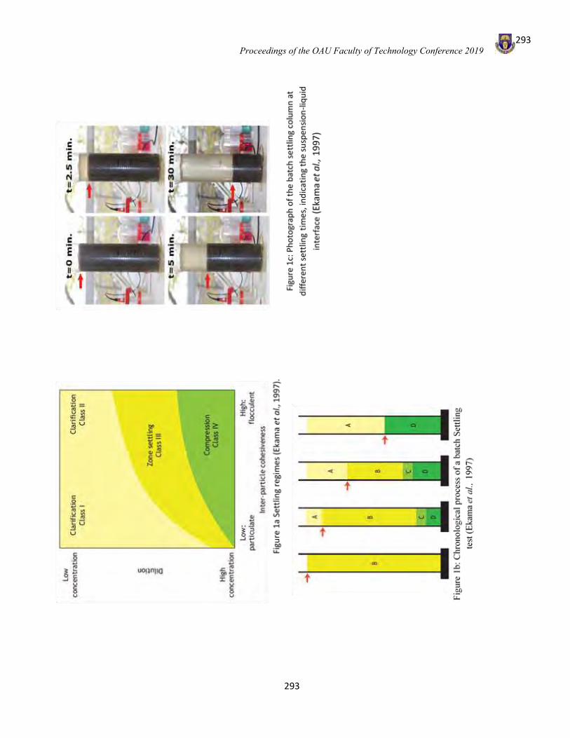
Proceedings of the OAU Faculty of Technology Conference 2019
293
293
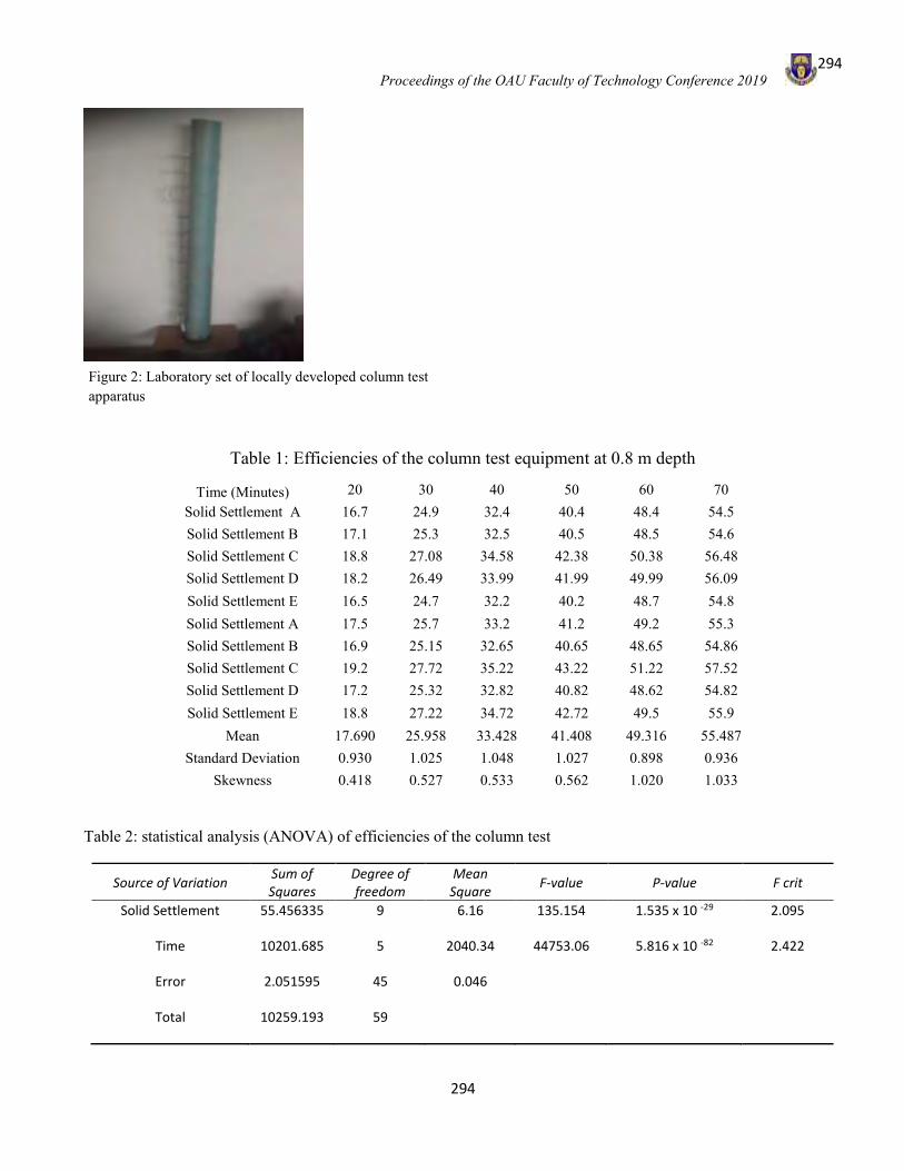
Proceedings of the OAU Faculty of Technology Conference 2019
294
294
Table 1: Efficiencies of the column test equipment at 0.8 m depth
Time (Minutes) 20 30 40 50 60 70 Solid Settlement A 16.7 24.9 32.4 40.4 48.4 54.5 Solid Settlement B 17.1 25.3 32.5 40.5 48.5 54.6 Solid Settlement C 18.8 27.08 34.58 42.38 50.38 56.48 Solid Settlement D 18.2 26.49 33.99 41.99 49.99 56.09 Solid Settlement E 16.5 24.7 32.2 40.2 48.7 54.8 Solid Settlement A 17.5 25.7 33.2 41.2 49.2 55.3 Solid Settlement B 16.9 25.15 32.65 40.65 48.65 54.86 Solid Settlement C 19.2 27.72 35.22 43.22 51.22 57.52 Solid Settlement D 17.2 25.32 32.82 40.82 48.62 54.82 Solid Settlement E 18.8 27.22 34.72 42.72 49.5 55.9
Mean 17.690 25.958 33.428 41.408 49.316 55.487 Standard Deviation 0.930 1.025 1.048 1.027 0.898 0.936
Skewness 0.418 0.527 0.533 0.562 1.020 1.033
Table 2: statistical analysis (ANOVA) of efficiencies of the column test
Source of Variation Sum of Squares
Degree of freedom
Mean Square
F-value P-value F crit
Solid Settlement 55.456335 9 6.16 135.154 1.535 x 10 -29 2.095
Time 10201.685 5 2040.34 44753.06 5.816 x 10 -82 2.422
Error 2.051595 45 0.046
Total 10259.193 59
Figure 2: Laboratory set of locally developed column test apparatus
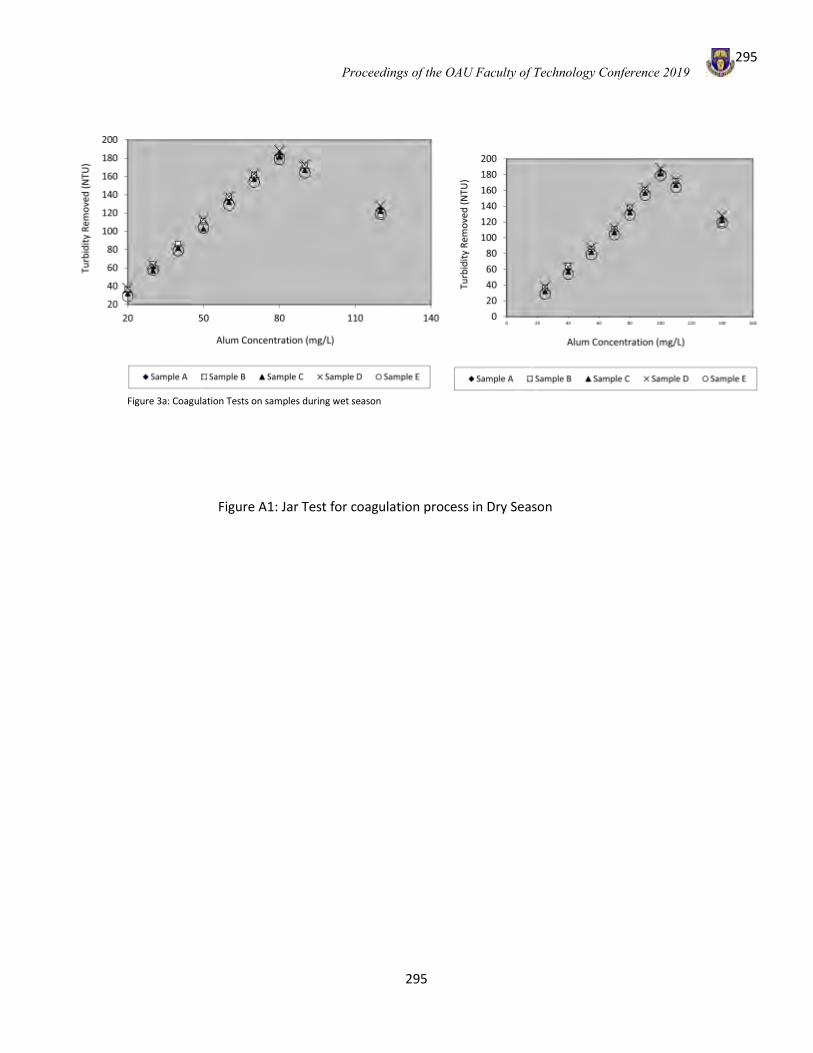
Proceedings of the OAU Faculty of Technology Conference 2019
295
295
Figure A1: Jar Test for coagulation process in Dry Season
Figure 3a: Coagulation Tests on samples during wet season
Figure 3b: Coagulation Tests on samples during dry season
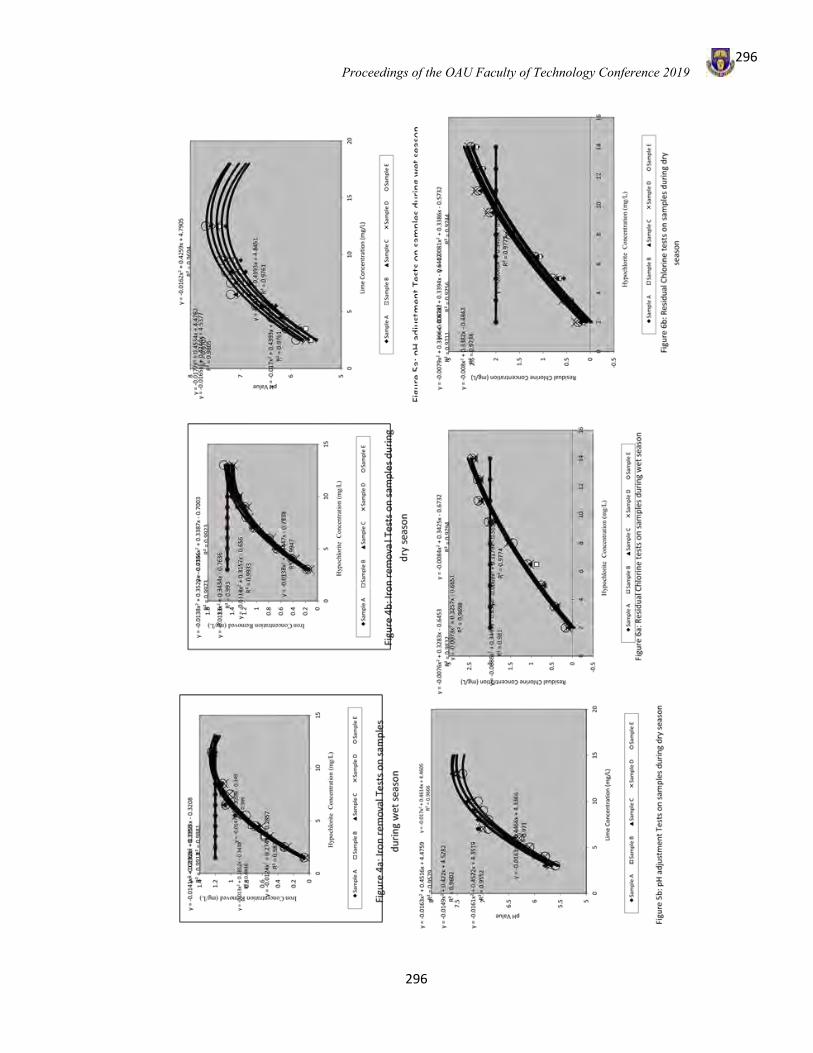
Proceedings of the OAU Faculty of Technology Conference 2019
296
296
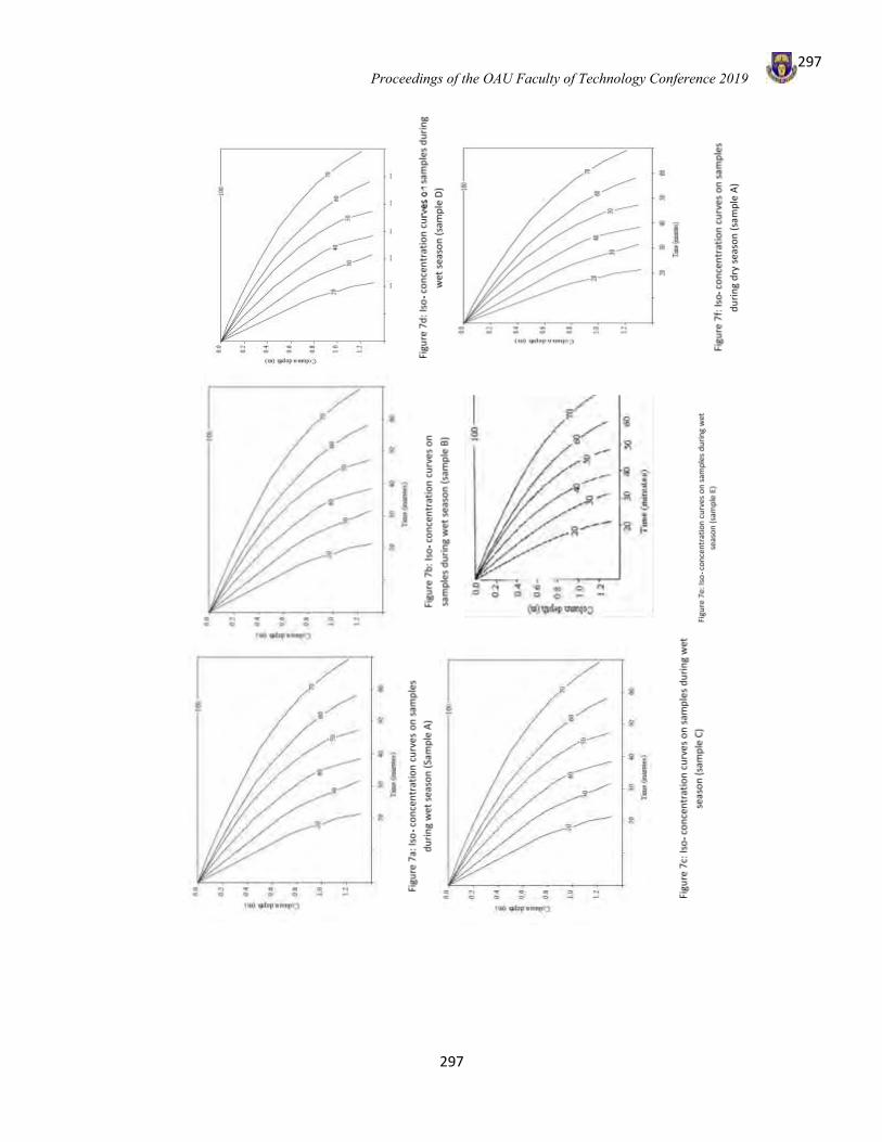
Proceedings of the OAU Faculty of Technology Conference 2019
297
297
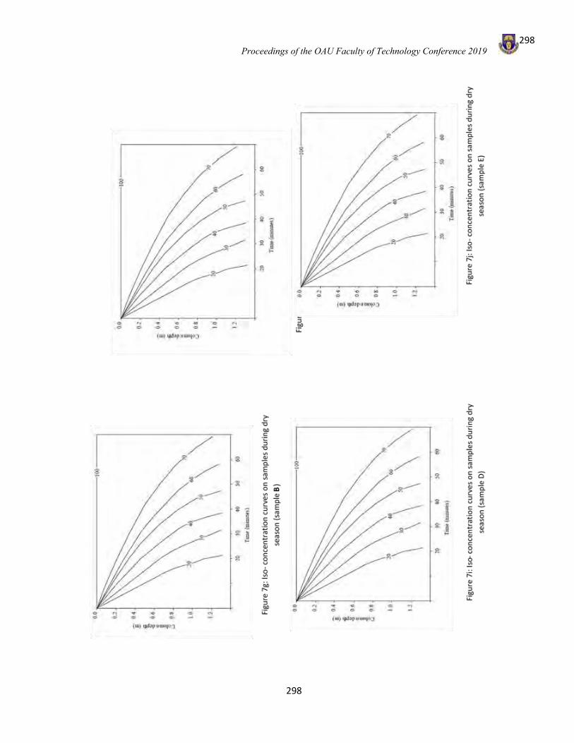
Proceedings of the OAU Faculty of Technology Conference 2019
298
298
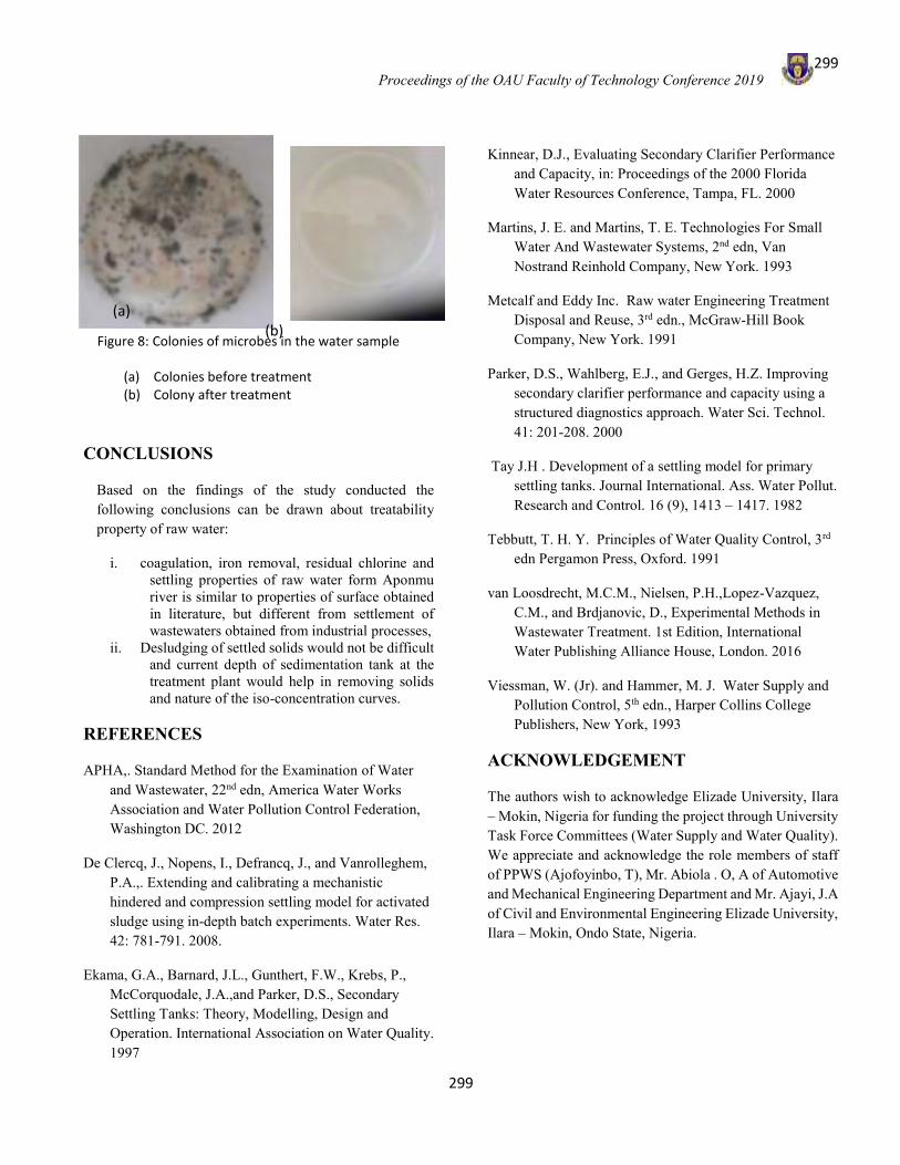
Proceedings of the OAU Faculty of Technology Conference 2019
299
299
CONCLUSIONS
Based on the findings of the study conducted the following conclusions can be drawn about treatability property of raw water:
i. coagulation, iron removal, residual chlorine and settling properties of raw water form Aponmu river is similar to properties of surface obtained in literature, but different from settlement of wastewaters obtained from industrial processes,
ii. Desludging of settled solids would not be difficult and current depth of sedimentation tank at the treatment plant would help in removing solids and nature of the iso-concentration curves.
REFERENCES
APHA,. Standard Method for the Examination of Water and Wastewater, 22nd edn, America Water Works Association and Water Pollution Control Federation, Washington DC. 2012
De Clercq, J., Nopens, I., Defrancq, J., and Vanrolleghem, P.A.,. Extending and calibrating a mechanistic hindered and compression settling model for activated sludge using in-depth batch experiments. Water Res. 42: 781-791. 2008.
Ekama, G.A., Barnard, J.L., Gunthert, F.W., Krebs, P., McCorquodale, J.A.,and Parker, D.S., Secondary Settling Tanks: Theory, Modelling, Design and Operation. International Association on Water Quality. 1997
Kinnear, D.J., Evaluating Secondary Clarifier Performance and Capacity, in: Proceedings of the 2000 Florida Water Resources Conference, Tampa, FL. 2000
Martins, J. E. and Martins, T. E. Technologies For Small Water And Wastewater Systems, 2nd edn, Van Nostrand Reinhold Company, New York. 1993
Metcalf and Eddy Inc. Raw water Engineering Treatment Disposal and Reuse, 3rd edn., McGraw-Hill Book Company, New York. 1991
Parker, D.S., Wahlberg, E.J., and Gerges, H.Z. Improving secondary clarifier performance and capacity using a structured diagnostics approach. Water Sci. Technol. 41: 201-208. 2000
Tay J.H . Development of a settling model for primary settling tanks. Journal International. Ass. Water Pollut. Research and Control. 16 (9), 1413 – 1417. 1982
Tebbutt, T. H. Y. Principles of Water Quality Control, 3rd edn Pergamon Press, Oxford. 1991
van Loosdrecht, M.C.M., Nielsen, P.H.,Lopez-Vazquez, C.M., and Brdjanovic, D., Experimental Methods in Wastewater Treatment. 1st Edition, International Water Publishing Alliance House, London. 2016
Viessman, W. (Jr). and Hammer, M. J. Water Supply and Pollution Control, 5th edn., Harper Collins College Publishers, New York, 1993
ACKNOWLEDGEMENT
The authors wish to acknowledge Elizade University, Ilara – Mokin, Nigeria for funding the project through University Task Force Committees (Water Supply and Water Quality). We appreciate and acknowledge the role members of staff of PPWS (Ajofoyinbo, T), Mr. Abiola . O, A of Automotive and Mechanical Engineering Department and Mr. Ajayi, J.A of Civil and Environmental Engineering Elizade University, Ilara – Mokin, Ondo State, Nigeria.
Figure 8: Colonies of microbes in the water sample
(a) Colonies before treatment (b) Colony after treatment
(a) (b)

Proceedings of the OAU Faculty of Technology Conference 2019
300
A STUDY ON ENERGY EFFICIENCY OF A MANUFACTURING COMPANY
A. O. Oke* and A. O. Oyeyemi Department of Mechanical Engineering, Obafemi Awolowo University, Ile-Ife
*Email of Corresponding Author: [email protected]
ABSTRACT The use of energy pervades every aspect of modern society but not efficient in many industries. Because of the incessant increase in fuel costs, energy efficiency study is becoming very important. This work thus studied the energy efficiency in a petrochemical company. The study utilizes preliminary energy audit, done for a period of 12 months (i.e. January – December, 2018). The preliminary energy audit was done based on the available data from the company obtained through oral interviews and secondary data sourced from the company's data book and Journal. The data collected are; monthly electrical energy consumed from the national grid, the quantity of diesel used to generate electricity monthly and the company’s monthly production rate over a period of the 12 months. The results show the percentage of electrical energy consumed from National Grid is 0.71%, whereas the percentage of electrical energy consumed as generated from Diesel Engine is 99.29%. The energy productivity decreased from 0.76314 MJ/kg to 0.65001 MJ/kg. An average of 85,984.45 MJ of energy was consumed monthly within this period, with an average production of 125.90 Mg. The average Energy Productivity, the average Intensity of Energy and the average Cost of Energy Input per unit kilogram are respectively; 0.68539 MJ/kg, 0.0099533 MJ/m2 and 109.52 kobo/kg. The average value of Normalized Performance Indicator (NPI) obtained is 1.33 MJ/m2 (0.00133 GJ/m2 = 0.3694 kWh/m2). NPI indicates the closeness of the energy used in a building to the optimum value. Keywords: Energy, productivity, consumption, energy efficiency, energy audit, electricity INTRODUCTION Energy is an integral component of a modern economy. It is an essential component in the production of all goods and services, but its use exerts heavy financial, environmental, and security costs. A key method of reducing energy costs while retaining its benefits is to use it more efficiently. Energy, in its different forms, is required as continuous input to all industrial processes. The total energy consumption of the industrial sectors of developed countries contributes to around 30-40% of total energy demand (Oyedepo and Aremu, 2013). In the last decade, there has been a greater awareness of the energy problems facing the world than at any other period in history. It is now widely accepted that the current rate of energy generation and supply cannot match the rapid growth in the rate of energy consumption (Adegoke and Bolaji, 1999; Momoh and Soaga, 1999). The importance of energy in sustained economic development is a well-accepted fact. Energy has always been an essential input to all aspects of the modern social life; it is indeed the life-wire in industrial production (Garba, 1999). Over the centuries, man has used various sources of energy in order to meet the basic essentials of life. Currently, fossil fuels provide the bulk of the world’s primary sources of energy, with hydro-electricity providing about 2% and nuclear fission, wood and other sources each accounting for 1% of the primary industrial energy used in the world (Aiyedun and Ologunye, 2001). Since fossil fuels are non-renewable natural resources, their reserve may soon get completely depleted (Garba et al., 1999). Present energy sources are yielding energy with increasing difficulty. Each unit of energy resource costs more to find, exploit and refine.
Energy conservationists are battling offshore exploration efforts, the installation of new pipelines, and construction of refineries and nuclear plants, and these make the job of satisfying our ever-increasing demand for energy more difficult. Hence, energy studies, analysis and audits are done in order to increase efficiency in energy utilization. Energy audit is a review of the total energy used and costs, normally performed in conjunction with a site investigation. It involves the classification of the energy sources and their contribution in running the factory. It provides a structural review of how energy is being purchased, managed and used with the aim of identifying opportunities for energy cost saving through improved services. It also gives the estimate of potential annual energy savings with implementation costs and pay back periods.
METHODOLOGY Study Area The company surveyed in this study is Moye Oil and Petrochemical Production Limited, located at km 3, Iwo-Ibadan Road, Osogbo, Osun State, South Western Nigeria. Moye has a team of professional with academic and practical exposure in oil blending and marketing. The company is typically an Oil Production and Refinery Company with a total yearly output of 1,510.83 Mg (Mega-gram) of various products. The company produces various kinds of oil products with different brand names and for different purposes. The products are; BRAVOL X & BRAVOL DX, MORDRAL AW

Proceedings of the OAU Faculty of Technology Conference 2019
301
SERIES, EXERGY 5000, MAROL 2T, PIXEL XM SUPER, ROLUBE. The raw materials for the Oil Production are base oil and additives. While the floor area of the company is 8640000 square meters. The main sources of energy for the plants are electrical and diesel fuel. The main and primary sources of electrical energy are the national grid and the self-generated power. Numerical data collection and analysis A Data were collected from the company through the following methods; On-site study of the operations. Oral interviews. Secondary data, sourced from the company's data book and Journal. Data collected include: (a) Electrical energy consumed from the national grid and the quantity of diesel used to generate electricity monthly over a period of 12 months of the year 2018. (b) Monthly production rate of the company over the period of 12 months. The flow process of the company is depicted in the Figure 1:
Figure 1: Flow Process of Production at Moye Oil and Petrochemical Limited.
Energy Evaluation The energy evaluations were carried out as outlined below. Total energy consumed Total enrgy consumed is the summation of the amount of electricity derived from the national grid and the diesel engine. Intensity of energy This is defined as the ratio of annual energy consumed (input) in MJ to the company floor area in m2 (Aiyedun et al., 2008), i.e. Intensity of energy (MJ/m2) = …………………………..(1) Energy productivity This is the total energy consumed (Input) per unit production (Output) (Aiyedun et al., 2008), i.e. Energy Productivity = ……………………..(2) Cost of energy input into a unit product This is represented mathematically as;
……………….…(3) The total energy cost is going to be calculated for the different energy sources based on their respective rates and summed up (Aiyedun et al., 2008). Normalized performance indicator (NPI) The normalized performance indicator (NPI) is a useful parameter in assessing the energy performance of a building. It is the total energy consumed divided by total floor area and multiplied by the hours of use factor value. (Aiyedun et al., 2008). A building with good rating will require further investigation, unless there are no obvious areas of improvement. Favourable rated buildings may deteriorate or the general standard may increase from time to time such that constant monitoring is required by the energy engineer in order to maintain good standard for the building at all times (Aiyedun et al., 2008). NPI = ……..(4)
Depot
Company(Farm Tanks)
Blendi-ng
Vessel
Finish Product Tanks (FPT)
Packaging
Heating Machine
Corking Machine
Filling Machine
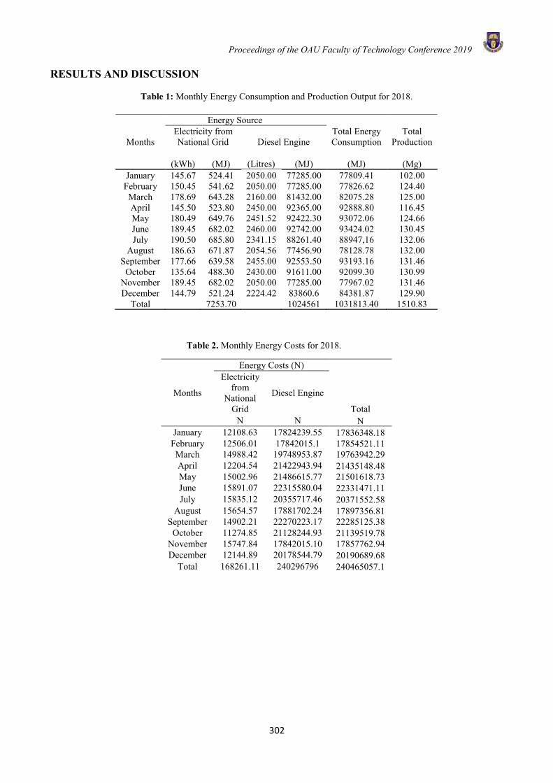
Proceedings of the OAU Faculty of Technology Conference 2019
302
RESULTS AND DISCUSSION
Table 1: Monthly Energy Consumption and Production Output for 2018.
Table 2. Monthly Energy Costs for 2018.
Energy Source Total
Production Months Electricity from National Grid Diesel Engine
Total Energy Consumption
(kWh) (MJ) (Litres) (MJ) (MJ) (Mg)
January 145.67 524.41 2050.00 77285.00 77809.41 102.00 February 150.45 541.62 2050.00 77285.00 77826.62 124.40 March 178.69 643.28 2160.00 81432.00 82075.28 125.00 April 145.50 523.80 2450.00 92365.00 92888.80 116.45 May 180.49 649.76 2451.52 92422.30 93072.06 124.66 June 189.45 682.02 2460.00 92742.00 93424.02 130.45 July 190.50 685.80 2341.15 88261.40 88947,16 132.06
August 186.63 671.87 2054.56 77456.90 78128.78 132.00 September 177.66 639.58 2455.00 92553.50 93193.16 131.46
October 135.64 488.30 2430.00 91611.00 92099.30 130.99 November 189.45 682.02 2050.00 77285.00 77967.02 131.46 December 144.79 521.24 2224.42 83860.6 84381.87 129.90
Total 7253.70 1024561 1031813.40 1510.83
Months
Energy Costs (N) Electricity
from National
Grid
Diesel Engine
Total N N N
January 12108.63 17824239.55 17836348.18 February 12506.01 17842015.1 17854521.11 March 14988.42 19748953.87 19763942.29 April 12204.54 21422943.94 21435148.48 May 15002.96 21486615.77 21501618.73 June 15891.07 22315580.04 22331471.11 July 15835.12 20355717.46 20371552.58
August 15654.57 17881702.24 17897356.81 September 14902.21 22270223.17 22285125.38
October 11274.85 21128244.93 21139519.78 November 15747.84 17842015.10 17857762.94 December 12144.89 20178544.79 20190689.68
Total 168261.11 240296796 240465057.1

Proceedings of the OAU Faculty of Technology Conference 2019
303
Energy productivity was calculated for the 12 months for each of the energy sources (National Grid and Diesel Engine) and the total combination of the two energy sources and the results for each is illustrated in Figure 2
Figure 2: Energy Productivity (MJ/kg) for the use of the total sources of energy The intensity of energy was calculated for the period of 12 months and illustrated in Figure 3
Figure 3: Intensity of Energy for the use of the total sources of energy. The total energy cost was calculated for the different energy sources based on their respective rates and summed up and presented in Figure 4. The values of the price variation across each month for each of the energy sources per unit value as at the time of this audit are given as 1kWh (from National Grid) = N23.09 and N23.30, while 1 litre (of Diesel Oil) = N230.63, N230.86 and N240.62.
Figure 4: Cost of Energy Input for the use of the total sources of energy.
The hours of use factor of electricity per day vary for each of the energy sources across the months; 3.93 hours, 6.85 hours and 8.78 hours (for national grid) and 2.22 hours, 4.15 hours and 7.03 hours (for the generating set). The NPI for the period under consideration is presented in Figure 5.
Figure 5: Normalized Performance Indicator (NPI) for the use of the total source of energy. Analysis of results presented above showed that, the highest monthly energy consumption recorded in the company for each of the energy sources are; 685.80MJ in July (National Grid) and 92742.00 MJ in June (Diesel Engine), and the least monthly energy consumption are; 521.24 MJ in December (National Grid) and 102.00 MJ in January (Diesel Engine) with the total average values of; 604.48 MJ (National Grid) and 85380.08 MJ (Diesel Engine), whereby the total highest production recorded in the company in the year, 2018 is 132.06Mg. The least energy consumed was electricity from the National Grid (National Grid) accounting for 0.71% on the average, while diesel duel energy expended in operating Diesel Engine was the highest consumed source of energy and it accounted for 99.29% on average, as indicated in Table 3.
00.20.40.60.8
1
Jan
uar
y
Feb
ruar
y
Mar
ch
Ap
ril
May
Jun
e
July
Au
gust
Sep
tem
ber
Oct
ob
er
No
vem
ber
Dec
em
ber
Ener
gyPr
oduc
tivity
MJ/
kg
Period (Time of the year)
0.0080.009
0.010.011
Inte
nsity
of
Ener
gyM
J/m
2
Period (Time of the year)
050
100150200
Jan
uar
y
Feb
ruar
y
Mar
ch
Ap
ril
May
Jun
e
July
Au
gust
Sep
tem
ber
Oct
ob
er
No
vem
ber
De
cem
be
r
Cos
t of E
nerg
y In
put…
Period (Time of the year)
0123
Jan
uar
y
Feb
ruar
y
Mar
ch
Ap
ril
May
Jun
e
July
Au
gust
Septem…
Oct
ob
er
Novemb…
Decem
b…
Nor
mal
ized
Perf
orm
ance
Indi
cato
r…
Period (Time of the year)

Proceedings of the OAU Faculty of Technology Conference 2019
304
Table 3. Summary of the Percentage of Total Energy Consumed Energy Source
Total Energy Consumed (%)
Average (Jan. - Dec.)
Jan. Feb. Mar. Apr. May Jun. Jul. Aug. Sep. Oct. Nov. Dec. National Grid
0.67 0.70 0.78 0.56 0.70 0.73 0.77 0.86 0.69 0.53 0.87 0.62 0.71
Diesel Engine
99.33 99.30 99.22 99.44 99.30 99.27 99.23 99.14 99.31 99.47 99.13 99.38 99.29
Discussion and Conclusions The sources of energy in the company surveyed comprise of electricity from the National Grid and fossil fuel (Diesel) for generating set (Diesel Engine). The pattern of energy consumption in the company is mainly from the diesel engine generating set. The results of the analysis and audit made over the period of 12 months in 2018 for a treated floor area of 8640000m2 showed that the percentage of electrical energy consumed (from National Grid) is 0.71%, whereas the percentage of electrical energy consumed (from Diesel Engine) is 99.29%. The energy productivity decreased essentially from 0.76314 MJ/kg in January to 0.65001 MJ/kg in December. An average of 85,984.45 MJ of energy was consumed monthly within this period (the 12 months of 2018), with an average production of 125.90 Mg. The average Energy Productivity, the average Intensity of Energy and the average Cost of Energy Input per unit kilogram are respectively; 0.68539 MJ/kg, 0.0099533 MJ/m2 and 109.52 kobo/kg. The average value of Normalized Performance Indicator (NPI) obtained is 1.33 MJ/m2 (0.00133 GJ/m2 = 0.3694 kWh/m2). Therefore, it shows the ineffective utilization of energy in the company. This implies that more energy is consumed or expended in the production of the finished product or output, the energy productivity within the period of study for the two energy sources (electricity from national grid and diesel engine) and their total are less than unit. In order to still prevent unnecessary wastage of energy and to lower the cost of energy consumption, the following factors must be carefully and critically looked into:
Procurement of test equipment for energy monitoring in the company.
Significant capital investment to improve the energy consumption.
Detailed audit, if possible, should still further be used to identify the causes of energy wastes.
Proper maintenance and control must be done in order to improve the energy productivity.
The company should engage in the procurement of more modern energy efficient equipment to carry out their production.
The company should be enlightened and engage more in learning about various programs on energy efficiency study.
REFERENCES Adegoke, C.O. and Bolaji, B.O. (1999): “Exergetic
analysis of thermosyphon solar water heating systems,” Nigerian Journal of Renewable Energy, vol. 7, No. 1 & 2, pp. 50 – 54.
Aiyedun, P. O., Adeyemi, O. A. and Bolaji, B. O. (2008): “Energy Efficiency of a Manufacturing Industry: A Case Study of Nigeria Eagle Flour Mills Limited, Ibadan,” ASSET Series B, vol. 7, No. 2, pp. 91-103.
Aiyedun, P.O. and Ologunye, O.B. (2001): “Energy Efficiency of a private sector with Cadbury Nigeria Plc, Ikeja, Lagos as a case study,” NSE Technical Transactions, vol. 36, No. 2, pp. 59 – 66.
Garba, B., Sambo, A.S., Danshehu, B.G. (1995): “Effect of some operating parameters on biogas production,” Renewable Energy, vol. 6, pp. 343 – 347.
Garba, B. (1999): “Mechanisms and biochemistry of methanogenesis in biogas production,” Nigerian Journal of Renewable Energy, vol. 7, . 1 & 2, pp. 12 – 16.
Momoh, S. and Soaga, J. (1999): “Biomass energy consumption in Nigeria: Integrating demand and supply,” Nigerian Journal of Renewable Energy, vol. 7, No. 1 & 2, pp. 78 – 82.
Oyedepo, S. O. and Aremu, T. O. (2013): “Energy Audit of Manufacturing and processing Industries in Nigeria: A Case Study of Food Processing Industry and Distillation & Bottling Company,” American Journal of Energy Research, vol. 1, No. 3, pp. 36-44.
Proceedings of the OAU Faculty of Technology Conference 2019
305
PERFORMANCE COMPARISON OF THREAT CLASSIFICATION MODELS FOR CYBER-SITUATION AWARENESS
S. S. Olofintuyi1,* T. O. Omotehinwa1, O. H. Odukoya2 and E. A. Olajubu2
1Department of Mathematical Sciences, Achievers University Owo, Ondo, Nigeria
2Department of Computer Science, Obafemi Awolowo University, Ile-Ife, Osun, Nigeria
*Email of Corresponding Author: [email protected]
ABSTRACT Cyber threats are becoming an issue and a great threat to organizations that work with data, and millions of dollars are being lost to hackers. Various machine learning algorithms have been used to detect threat at the first phase of situation awareness model. In this paper, we compare the performance of Support Vector Machine (SVM) and Artificial Neural Network (ANN) at the perception phase of situation awareness model. Feature selection was used to extract the most significant attributes and they are fed to ANN and SVM. Knowledge Discovery and Data Mining (KDD 99) dataset was used during the training of the two proposed algorithms. At the end of the simulation, ANN gives an accuracy of 0.978 while SVM gives an accuracy of 0.957. The results of the simulation showed that ANN is more accurate in comparison to SVM for threat detection on a computer network.
Keywords: Situation Awareness, Intrusion Detection System, Artificial Neural Network, Support Vector Machine,
performance comparison.
INTRODUCTION According to Endsley (1995) Situation Awareness (SA) is the act of detection of threat in the environment and relaying it back to the system administrator. Generally, the model for threat detection are classified into three sections which are the perception phase, comprehension phase and projection phase. The perception phase is solely responsible for detection of threat while the comprehension phase is connected to a trained database of various events of historical database that has been trained by the network administrator. Once the comprehension phase has finished judging whether such event is malicious or not, the projection phase then sends the feedback to the comprehension phase. A threat is a group of malicious programs that intrudes into one’s program. Existing models for monitoring and protecting computer networks are unable to accurately detect modern threats and intrusions such as Denial of service (DOS), User to root, Root to local and probing. The need for an efficient classifier or predictive model for intrusion detection is on the increase as a result of the emergences of big data (Othman, et al., 2018) and enterprise migrations to the cloud. Intruders are gaining more grounds due to the imbalances in the cyber security. This has negatively affected organization that keeps sensitive data, most organization have paid heavily for this and vital information has been lost to intruders. According to Dutt, et al., 2012) they also worked on SA where an instance based learning theory was used for prediction of threat on a computer network. Furthermore,
Mitchell, (1997) make use of Naïve Bayes Classifier for classifying whether a class is threat or non-threat on a computer network . Finally, Prahlad and Wenke (2006) make use of statistical approach for detecting threat on SA but it was observed that the approach cannot give accurate prediction to the administrator. Researcher has used various algorithms on the network for threat detection, but none has been able to obtain 100% accuracy. Feature selection is defined as the removal of redundant attributes from a given dataset (Yildirim, 2015). While on the other hand, machine learning is a branch of Artificial Intelligence that uses statistical and optimization techniques to create computers intelligent machines. This study is targeted at comparing two of the machine learning techniques that are widely used due to their attributes that have given them edge over other supervised machine learning algorithms. Mehibs and Hashim, (2018) proposed an intrusion detection system based on back propagation neural network. The back propagation relies on the modification of weight to train the system; this is subsequently used to forecast the class label of the new input patterns. The authors proposed an algorithm for the classification of DOS, U2R, Probe and R2L and the developed algorithm was evaluated with Knowledge Discovery and Data Mining (KDD 99) dataset. The study obtained a detection rate of 0.99 and false alarm rate of 0.03 with a data size of 500. With 200% increase in data size, the results obtained
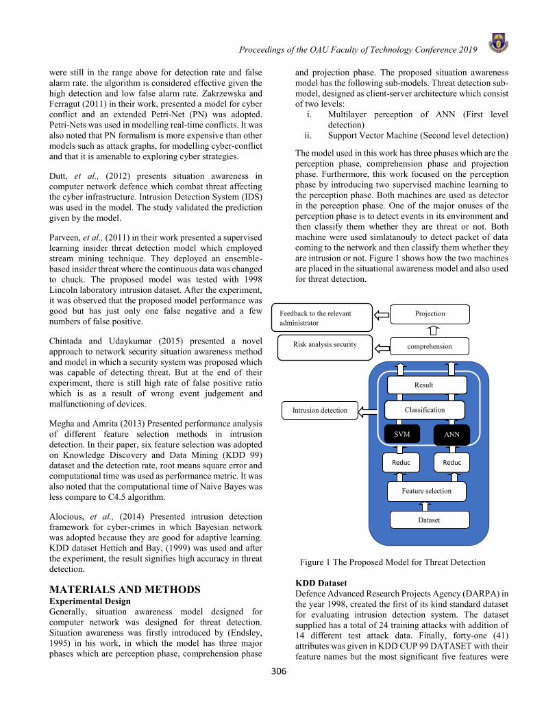
Proceedings of the OAU Faculty of Technology Conference 2019
306
were still in the range above for detection rate and false alarm rate. the algorithm is considered effective given the high detection and low false alarm rate. Zakrzewska and Ferragut (2011) in their work, presented a model for cyber conflict and an extended Petri-Net (PN) was adopted. Petri-Nets was used in modelling real-time conflicts. It was also noted that PN formalism is more expensive than other models such as attack graphs, for modelling cyber-conflict and that it is amenable to exploring cyber strategies.
Dutt, et al., (2012) presents situation awareness in computer network defence which combat threat affecting the cyber infrastructure. Intrusion Detection System (IDS) was used in the model. The study validated the prediction given by the model.
Parveen, et al., (2011) in their work presented a supervised learning insider threat detection model which employed stream mining technique. They deployed an ensemble-based insider threat where the continuous data was changed to chuck. The proposed model was tested with 1998 Lincoln laboratory intrusion dataset. After the experiment, it was observed that the proposed model performance was good but has just only one false negative and a few numbers of false positive.
Chintada and Udaykumar (2015) presented a novel approach to network security situation awareness method and model in which a security system was proposed which was capable of detecting threat. But at the end of their experiment, there is still high rate of false positive ratio which is as a result of wrong event judgement and malfunctioning of devices.
Megha and Amrita (2013) Presented performance analysis of different feature selection methods in intrusion detection. In their paper, six feature selection was adopted on Knowledge Discovery and Data Mining (KDD 99) dataset and the detection rate, root means square error and computational time was used as performance metric. It was also noted that the computational time of Naive Bayes was less compare to C4.5 algorithm.
Alocious, et al., (2014) Presented intrusion detection framework for cyber-crimes in which Bayesian network was adopted because they are good for adaptive learning. KDD dataset Hettich and Bay, (1999) was used and after the experiment, the result signifies high accuracy in threat detection.
MATERIALS AND METHODS Experimental Design Generally, situation awareness model designed for computer network was designed for threat detection. Situation awareness was firstly introduced by (Endsley, 1995) in his work, in which the model has three major phases which are perception phase, comprehension phase
and projection phase. The proposed situation awareness model has the following sub-models. Threat detection sub-model, designed as client-server architecture which consist of two levels:
i. Multilayer perception of ANN (First level detection)
ii. Support Vector Machine (Second level detection)
The model used in this work has three phases which are the perception phase, comprehension phase and projection phase. Furthermore, this work focused on the perception phase by introducing two supervised machine learning to the perception phase. Both machines are used as detector in the perception phase. One of the major onuses of the perception phase is to detect events in its environment and then classify them whether they are threat or not. Both machine were used simlatanouly to detect packet of data coming to the network and then classify them whether they are intrusion or not. Figure 1 shows how the two machines are placed in the situational awareness model and also used for threat detection.
Figure 1 The Proposed Model for Threat Detection KDD Dataset Defence Advanced Research Projects Agency (DARPA) in the year 1998, created the first of its kind standard dataset for evaluating intrusion detection system. The dataset supplied has a total of 24 training attacks with addition of 14 different test attack data. Finally, forty-one (41) attributes was given in KDD CUP 99 DATASET with their feature names but the most significant five features were
Dataset (KDD)
Feature selection
Reduc
ed
Reduc
ed
Projection
Intrusion detection
comprehension
Feedback to the relevant administrator
Risk analysis security
SVM ANN
Classification
Result
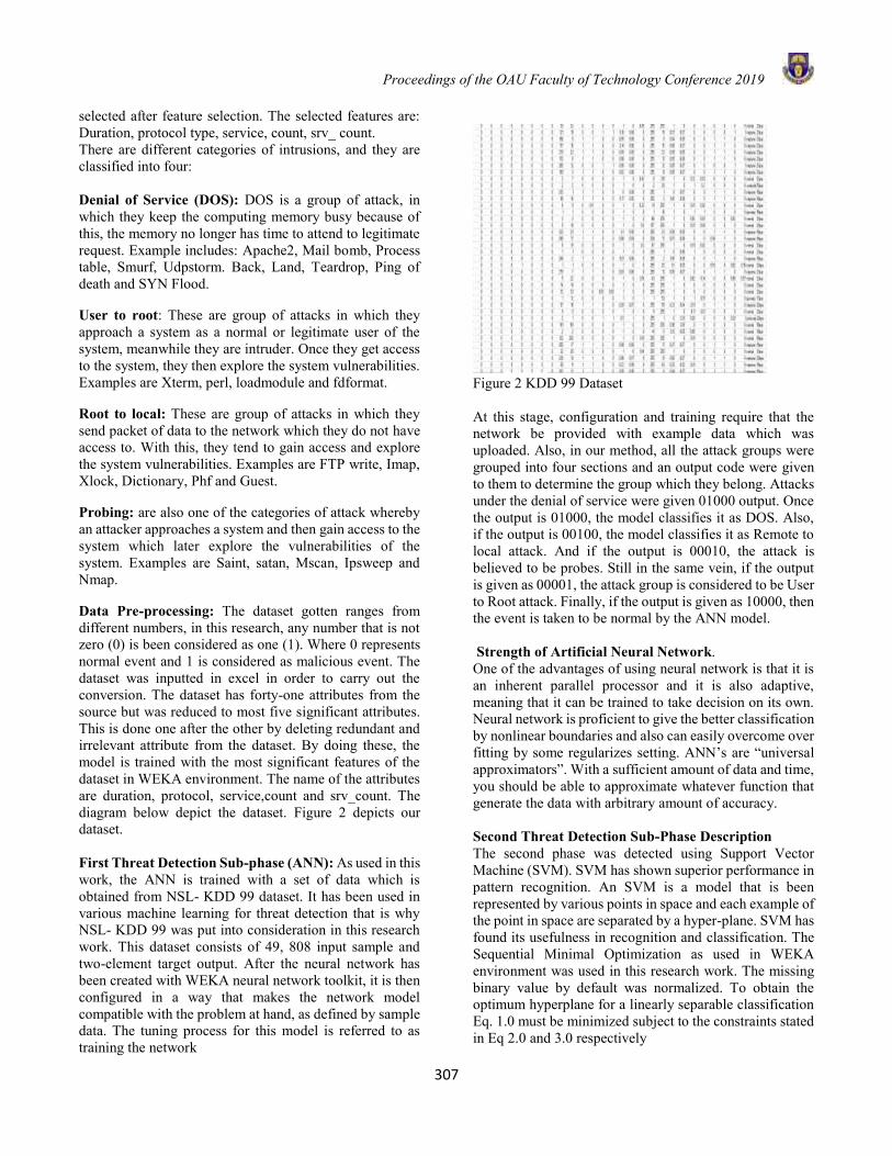
Proceedings of the OAU Faculty of Technology Conference 2019
307
selected after feature selection. The selected features are: Duration, protocol type, service, count, srv_ count. There are different categories of intrusions, and they are classified into four: Denial of Service (DOS): DOS is a group of attack, in which they keep the computing memory busy because of this, the memory no longer has time to attend to legitimate request. Example includes: Apache2, Mail bomb, Process table, Smurf, Udpstorm. Back, Land, Teardrop, Ping of death and SYN Flood.
User to root: These are group of attacks in which they approach a system as a normal or legitimate user of the system, meanwhile they are intruder. Once they get access to the system, they then explore the system vulnerabilities. Examples are Xterm, perl, loadmodule and fdformat.
Root to local: These are group of attacks in which they send packet of data to the network which they do not have access to. With this, they tend to gain access and explore the system vulnerabilities. Examples are FTP write, Imap, Xlock, Dictionary, Phf and Guest.
Probing: are also one of the categories of attack whereby an attacker approaches a system and then gain access to the system which later explore the vulnerabilities of the system. Examples are Saint, satan, Mscan, Ipsweep and Nmap.
Data Pre-processing: The dataset gotten ranges from different numbers, in this research, any number that is not zero (0) is been considered as one (1). Where 0 represents normal event and 1 is considered as malicious event. The dataset was inputted in excel in order to carry out the conversion. The dataset has forty-one attributes from the source but was reduced to most five significant attributes. This is done one after the other by deleting redundant and irrelevant attribute from the dataset. By doing these, the model is trained with the most significant features of the dataset in WEKA environment. The name of the attributes are duration, protocol, service,count and srv_count. The diagram below depict the dataset. Figure 2 depicts our dataset. First Threat Detection Sub-phase (ANN): As used in this work, the ANN is trained with a set of data which is obtained from NSL- KDD 99 dataset. It has been used in various machine learning for threat detection that is why NSL- KDD 99 was put into consideration in this research work. This dataset consists of 49, 808 input sample and two-element target output. After the neural network has been created with WEKA neural network toolkit, it is then configured in a way that makes the network model compatible with the problem at hand, as defined by sample data. The tuning process for this model is referred to as training the network
Figure 2 KDD 99 Dataset At this stage, configuration and training require that the network be provided with example data which was uploaded. Also, in our method, all the attack groups were grouped into four sections and an output code were given to them to determine the group which they belong. Attacks under the denial of service were given 01000 output. Once the output is 01000, the model classifies it as DOS. Also, if the output is 00100, the model classifies it as Remote to local attack. And if the output is 00010, the attack is believed to be probes. Still in the same vein, if the output is given as 00001, the attack group is considered to be User to Root attack. Finally, if the output is given as 10000, then the event is taken to be normal by the ANN model. Strength of Artificial Neural Network. One of the advantages of using neural network is that it is an inherent parallel processor and it is also adaptive, meaning that it can be trained to take decision on its own. Neural network is proficient to give the better classification by nonlinear boundaries and also can easily overcome over fitting by some regularizes setting. ANN’s are “universal approximators”. With a sufficient amount of data and time, you should be able to approximate whatever function that generate the data with arbitrary amount of accuracy. Second Threat Detection Sub-Phase Description The second phase was detected using Support Vector Machine (SVM). SVM has shown superior performance in pattern recognition. An SVM is a model that is been represented by various points in space and each example of the point in space are separated by a hyper-plane. SVM has found its usefulness in recognition and classification. The Sequential Minimal Optimization as used in WEKA environment was used in this research work. The missing binary value by default was normalized. To obtain the optimum hyperplane for a linearly separable classification Eq. 1.0 must be minimized subject to the constraints stated in Eq 2.0 and 3.0 respectively
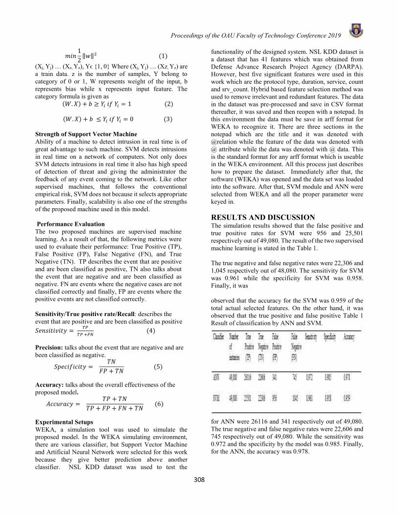
Proceedings of the OAU Faculty of Technology Conference 2019
308
𝑚𝑖𝑛1
2‖𝑤‖2 (1)
(Xj, Yj) … (Xz, Yz), Yϵ 1, 0 Where (Xj, Yj) … (Xz, Yz) are a train data. z is the number of samples, Y belong to category of 0 or 1, W represents weight of the input, b represents bias while x represents input feature. The category formula is given as
(𝑊. 𝑋) + 𝑏 ≥ 𝑌𝑖 𝑖𝑓 𝑌𝑖 = 1 (2)
(𝑊. 𝑋) + 𝑏 ≤ 𝑌𝑖 𝑖𝑓 𝑌𝑖 = 0 (3) Strength of Support Vector Machine Ability of a machine to detect intrusion in real time is of great advantage to such machine. SVM detects intrusions in real time on a network of computers. Not only does SVM detects intrusions in real time it also has high speed of detection of threat and giving the administrator the feedback of any event coming to the network. Like other supervised machines, that follows the conventional empirical risk, SVM does not because it selects appropriate parameters. Finally, scalability is also one of the strengths of the proposed machine used in this model. Performance Evaluation The two proposed machines are supervised machine learning. As a result of that, the following metrics were used to evaluate their performance: True Positive (TP), False Positive (FP), False Negative (FN), and True Negative (TN). TP describes the event that are positive and are been classified as positive, TN also talks about the event that are negative and are been classified as negative. FN are events where the negative cases are not classified correctly and finally, FP are events where the positive events are not classified correctly. Sensitivity/True positive rate/Recall: describes the event that are positive and are been classified as positive 𝑆𝑒𝑛𝑠𝑖𝑡𝑖𝑣𝑖𝑡𝑦 =
𝑇𝑃
𝑇𝑃 +𝐹𝑁 (4)
Precision: talks about the event that are negative and are been classified as negative.
𝑆𝑝𝑒𝑐𝑖𝑓𝑖𝑐𝑖𝑡𝑦 = 𝑇𝑁
𝐹𝑃 + 𝑇𝑁 (5)
Accuracy: talks about the overall effectiveness of the proposed model.
𝐴𝑐𝑐𝑢𝑟𝑎𝑐𝑦 = 𝑇𝑃 + 𝑇𝑁
𝑇𝑃 + 𝐹𝑃 + 𝐹𝑁 + 𝑇𝑁 (6)
Experimental Setups WEKA, a simulation tool was used to simulate the proposed model. In the WEKA simulating environment, there are various classifier, but Support Vector Machine and Artificial Neural Network were selected for this work because they give better prediction above another classifier. NSL KDD dataset was used to test the
functionality of the designed system. NSL KDD dataset is a dataset that has 41 features which was obtained from Defense Advance Research Project Agency (DARPA). However, best five significant features were used in this work which are the protocol type, duration, service, count and srv_count. Hybrid based feature selection method was used to remove irrelevant and redundant features. The data in the dataset was pre-processed and save in CSV format thereafter, it was saved and then reopen with a notepad. In this environment the data must be save in arff format for WEKA to recognize it. There are three sections in the notepad which are the title and it was denoted with @relation while the feature of the data was denoted with @ attribute while the data was denoted with @ data. This is the standard format for any arff format which is useable in the WEKA environment. All this process just describes how to prepare the dataset. Immediately after that, the software (WEKA) was opened and the data set was loaded into the software. After that, SVM module and ANN were selected from WEKA and all the proper parameter were keyed in. RESULTS AND DISCUSSION The simulation results showed that the false positive and true positive rates for SVM were 956 and 25,501 respectively out of 49,080. The result of the two supervised machine learning is stated in the Table 1. The true negative and false negative rates were 22,306 and 1,045 respectively out of 48,080. The sensitivity for SVM was 0.961 while the specificity for SVM was 0.958. Finally, it was observed that the accuracy for the SVM was 0.959 of the total actual selected features. On the other hand, it was observed that the true positive and false positive Table 1 Result of classification by ANN and SVM.
for ANN were 26116 and 341 respectively out of 49,080. The true negative and false negative rates were 22,606 and 745 respectively out of 49,080. While the sensitivity was 0.972 and the specificity by the model was 0.985. Finally, for the ANN, the accuracy was 0.978.
Proceedings of the OAU Faculty of Technology Conference 2019
309
CONCLUSION After the experiment, it was discovered that ANN shows more accuracy than SVM for threat detection on a computer network. However, the differences between the two machines for threat detection was minimal but can’t be neglected. From this work, whenever a network administrator wants to build-up a system for awareness of intrusion on his network, ANN should be considered for accuracy in threat detection which also has a great advantage of speed in intrusion detection system. REFERENCES
Alocious, C., Abouzakhar, N., Xiao, H., Christianson, B., Intrusion detection system using Bayesian network modeling. In proceedings of the 13th European conference on cyber warfare and security, 3(1): 223-230, 2014.
Chintada, S., Udaykumar, J., A novel approach to network security situation awareness method and model. International Journal of Engineering and Innovative Technology (IJEIT), 4(11): 103-107, 2015.
Dutt,V., Ahn,Y., Gonzalez, S., Cyber Situation Awareness: Modelling the Security Analyst in a Cyber-Attack Scenario through Instance-based Learning. In proceeding of Data and Applications Security and Privacy. Heidelberg, Germany, 2012.
Endsley, M. R., Toward a theory of situation awareness in dynamic system. In Human Factors Journal, 37(1): 32-64, 1995.
Hettich, S., Bay, S. D., KDD Cup 1999 Data. Retrieved from The UCI KDD Archive: http://kdd.ics.uci.edu, 1999.
Megha, A., Amrita, K., Performance analysis of different feature selection methods in intrusion detection. International Journal of Scientific and Technology Research, 2(6): 225-231, 2013.
Mehibs, M. S., Hashim, H. S., Proposed Network Intrusion Detection System In Cloud
Environment Based on Back Propagation Neural Network. Journal of Babylon University, Pure and Applied Sciences, 26(1): 29-40, 2018.
Mitchell. T., Machine Learning, McGraw Hill.1997.
Othman, M. S., Ba-Alwi, M. F., Alsohybe, T. N., Al-Hashida, A. Y., Intrusion detection model using machine learning algorithm on Big Data environment. Journal of Big Data, 5(34): 250-261, 2018.
Parveen, P., Weger, Z. R., Thuraisingham, B., Hamlen, K., Khan, L. Supervised learning for insider threat detection using stream mining. In the proceedings of IEEE 23rd International conference on Tools with Artificial Intelligence ICTAI. Boca Raton, USA. 2011.
Prahlad, F., Wemke, L., Evaluating network anomaly detection systems: Formal seasoning and practical techniques. In Proceeding of the 15th USENIX Security Symposium, Vancouver, B.C., Canada, 2006.
Yildirim, P., Filter-Based Feature Selection Methods for Predicting of Risks in Hepatitis Disease. International Journal of Machine Learning and Computing, 5(4): 258-263, 2015.
Zakrzewska, A., Ferragut, E., Modelling Cyber Conflicts using an Extended Petri net Formalism In: Computational Intelligence in Cyber Security. IEEE Symposium. Califonia, USA, 43-46, 2011.
Proceedings of the OAU Faculty of Technology Conference 2019
310
SOLAR ACTIVITY EFFECT ON GPS-DERIVED IONOSPHERIC TOTAL ELECTRON CONTENT VARIATION AT LOW-LATITUDE STATIONS
L. G. Olatunbosun1, A. O. Olabode2,*, T. P. Owolabi3 and E. A. Ariyibi2 1Department of Science Technology,
Federal Polytechnic, Ado-Ekiti, Nigeria. 2Department of Physics and Engineering Physics, Obafemi Awolowo University, Ile-Ife, Nigeria.
3African Regional Centre for Space Science and Technology Education in English, Obafemi Awolowo University Campus, Ile-Ife, Nigeria.
*Email of Corresponding Author: [email protected]
ABSTRACT The dual frequency signals from the GPS satellites recorded at Ile-Ife, Nigeria (Geomagnetic Latitude 7.52° N, Longitude 4.28° E); Addis Ababa, Ethiopia (Geomagnetic Latitude 9.04° N, Longitude 38.77° E) and Bangalore, India (Geomagnetic Latitude 13.03° N, Longitude 77.57° E) have been analyzed to study the effects of solar activity on Total Electron Content (TEC) variations for the years 2011 and 2012. The variations of TEC at maximum and minimum conditions of solar radio flux (F10.7) and sunspot number (SSN) for the two years revealed that the magnitude of TEC is influenced by solar activity, with maximum solar indices corresponding to maximum TEC values and was dependent on season and geographic location. The best correlation was found between TEC and F10.7, with a highest value of 0.851 at Addis Ababa in 2011. The statistical analysis revealed that in 2011, the daily mean peak TEC increased by 0.298, 0.550 and 0.531 TEC units with each additional SFU of F10.7 in Ile-Ife, Addis Ababa and Bangalore respectively. The coefficient of determination values of 48.7%, 72.4% and 70.6% in the three stations indicates the level of variance in TEC due to F10.7. The standard deviation values of 7.514, 8.189 and 8.875 for Ile-Ife, Addis Ababa and Bangalore respectively for F10.7 shows that Ile-Ife had the best of its values concentrated around the mean while Bangalore had the least. Keywords: GPS, Total Electron Content, Solar Radio Flux, Sunspot Number, Low-latitude Ionosphere INTRODUCTION The ionosphere of the Earth is the upper part of the atmosphere where electrons and ions exist in sufficient quantity. This is mostly caused by the solar radiation which produces free electrons from existing atmospheric gases. The ionization at the equatorial and low latitudes is known to be high compared to relatively moderate ionization changes in the mid-latitude region. This is as a result of the larger fraction of solar energy absorbed within ±30° latitude zone, centred on the equator (Abdu, 2005). The level of ionospheric activity is described in terms of electron density, quantified by the number of electrons in a vertical column of cross-sectional area 1 m2, known as total electron content (TEC) of the medium (Klobuchar, 1991). The exploitation of trans-ionospheric communications in satellite, aircraft, and surface transportation system navigations require more precise estimation of the ionospheric delay error, which is in direct proportion to TEC, in the navigation signal due to free electrons and ions in the ionosphere. Exploitation of the dual frequency global positioning system (GPS) signals for studying ionospheric characteristics is of great interest due to the dispersive nature of the ionosphere at the frequency range of GPS signals. Olatunbosun and Ariyibi (2015) studied TEC
variation in the low latitudes of Ile-Ife, Addis Ababa and Bangalore stations, where comparative results revealed highest TEC variations at Addis Ababa, followed by Bangalore and least in Ile-Ife station. They also made an observation of complexity in the low-latitude ionosphere. In this study, we investigate the contributions of solar activities on TEC variation as a continuation to Olatunbosun and Ariyibi, 2015, using observations from GPS measurements. In order to study the influence of solar activities on ionospheric TEC variations, solar sunspot number (SSN) and solar radio flux (F10.7) which are the most frequently used indices to describe solar activity (Svalgaard and Hudson, 2010) were correlated with GPS-derived observations for 2011 and 2012 at three stations located in the Equatorial Ionization Anomaly (EIA) region. This was with the view to better understand ionization response to solar activity variations. MATERIALS AND METHODS Total electron content (TEC) data were obtained from GPS Scintillation Decision Aid (GPS-SCINDA) receiver situated at Obafemi Awolowo University, Ile-Ife, Nigeria (Geomagnetic Latitude 7.52° N, Longitude 4.28° E) while TEC was estimated from Receiver Independent Exchange (RINEX) data files which were obtained from
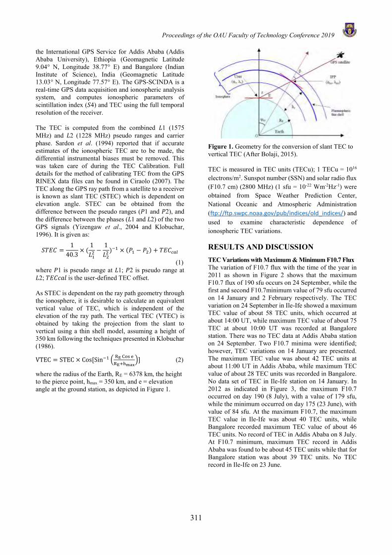
Proceedings of the OAU Faculty of Technology Conference 2019
311
the International GPS Service for Addis Ababa (Addis Ababa University), Ethiopia (Geomagnetic Latitude 9.04° N, Longitude 38.77° E) and Bangalore (Indian Institute of Science), India (Geomagnetic Latitude 13.03° N, Longitude 77.57° E). The GPS-SCINDA is a real-time GPS data acquisition and ionospheric analysis system, and computes ionospheric parameters of scintillation index (𝑆4) and TEC using the full temporal resolution of the receiver. The TEC is computed from the combined 𝐿1 (1575 MHz) and 𝐿2 (1228 MHz) pseudo ranges and carrier phase. Sardon et al. (1994) reported that if accurate estimates of the ionospheric TEC are to be made, the differential instrumental biases must be removed. This was taken care of during the TEC Calibration. Full details for the method of calibrating TEC from the GPS RINEX data files can be found in Ciraolo (2007). The TEC along the GPS ray path from a satellite to a receiver is known as slant TEC (STEC) which is dependent on elevation angle. STEC can be obtained from the difference between the pseudo ranges (𝑃1 and 𝑃2), and the difference between the phases (𝐿1 and 𝐿2) of the two GPS signals (Yizengaw et al., 2004 and Klobuchar, 1996). It is given as:
𝑆𝑇𝐸𝐶 =1
40.3× (
1
𝐿12 −
1
𝐿22)−1 × (𝑃1 − 𝑃2) + 𝑇𝐸𝐶𝑐𝑎𝑙
(1) where 𝑃1 is pseudo range at 𝐿1; 𝑃2 is pseudo range at 𝐿2; 𝑇𝐸𝐶𝑐𝑎𝑙 is the user-defined TEC offset. As STEC is dependent on the ray path geometry through the ionosphere, it is desirable to calculate an equivalent vertical value of TEC, which is independent of the elevation of the ray path. The vertical TEC (VTEC) is obtained by taking the projection from the slant to vertical using a thin shell model, assuming a height of 350 km following the techniques presented in Klobuchar (1986).
VTEC = STEC × Cos[Sin−1 (RE Cos e
RE+hmax)] (2)
where the radius of the Earth, RE = 6378 km, the height to the pierce point, hmax = 350 km, and e = elevation angle at the ground station, as depicted in Figure 1.
Figure 1. Geometry for the conversion of slant TEC to vertical TEC (After Bolaji, 2015). TEC is measured in TEC units (TECu); 1 TECu = 1016 electrons/m2. Sunspot number (SSN) and solar radio flux (F10.7 cm) (2800 MHz) (1 sfu = 10-22 Wm-2Hz-1) were obtained from Space Weather Prediction Center, National Oceanic and Atmospheric Administration (ftp://ftp.swpc.noaa.gov/pub/indices/old_indices/) and used to examine characteristic dependence of ionospheric TEC variations.
RESULTS AND DISCUSSION TEC Variations with Maximum & Minimum F10.7 Flux The variation of F10.7 flux with the time of the year in 2011 as shown in Figure 2 shows that the maximum F10.7 flux of 190 sfu occurs on 24 September, while the first and second F10.7minimum value of 79 sfu occurred on 14 January and 2 February respectively. The TEC variation on 24 September in Ile-Ife showed a maximum TEC value of about 58 TEC units, which occurred at about 14:00 UT, while maximum TEC value of about 75 TEC at about 10:00 UT was recorded at Bangalore station. There was no TEC data at Addis Ababa station on 24 September. Two F10.7 minima were identified; however, TEC variations on 14 January are presented. The maximum TEC value was about 42 TEC units at about 11:00 UT in Addis Ababa, while maximum TEC value of about 28 TEC units was recorded in Bangalore. No data set of TEC in Ile-Ife station on 14 January. In 2012 as indicated in Figure 3, the maximum F10.7 occurred on day 190 (8 July), with a value of 179 sfu, while the minimum occurred on day 175 (23 June), with value of 84 sfu. At the maximum F10.7, the maximum TEC value in Ile-Ife was about 40 TEC units, while Bangalore recorded maximum TEC value of about 46 TEC units. No record of TEC in Addis Ababa on 8 July. At F10.7 minimum, maximum TEC record in Addis Ababa was found to be about 45 TEC units while that for Bangalore station was about 39 TEC units. No TEC record in Ile-Ife on 23 June.
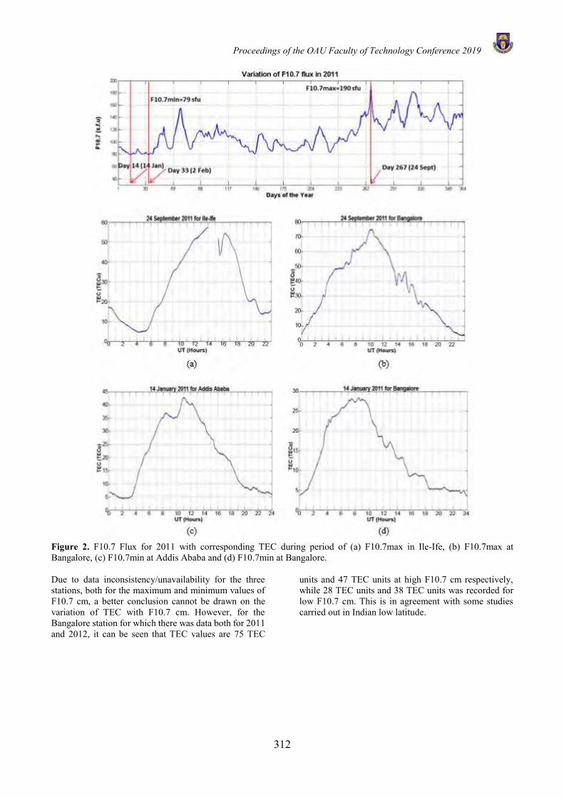
Proceedings of the OAU Faculty of Technology Conference 2019
312
Figure 2. F10.7 Flux for 2011 with corresponding TEC during period of (a) F10.7max in Ile-Ife, (b) F10.7max at Bangalore, (c) F10.7min at Addis Ababa and (d) F10.7min at Bangalore. Due to data inconsistency/unavailability for the three stations, both for the maximum and minimum values of F10.7 cm, a better conclusion cannot be drawn on the variation of TEC with F10.7 cm. However, for the Bangalore station for which there was data both for 2011 and 2012, it can be seen that TEC values are 75 TEC
units and 47 TEC units at high F10.7 cm respectively, while 28 TEC units and 38 TEC units was recorded for low F10.7 cm. This is in agreement with some studies carried out in Indian low latitude.
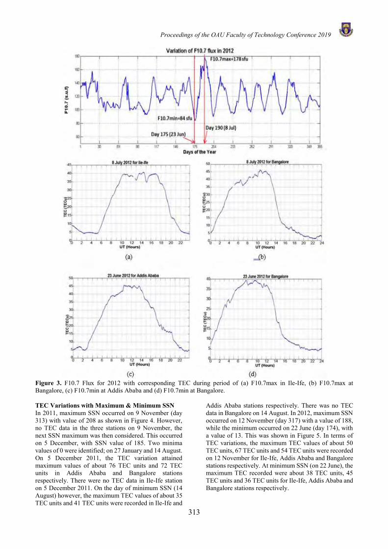
Proceedings of the OAU Faculty of Technology Conference 2019
313
Figure 3. F10.7 Flux for 2012 with corresponding TEC during period of (a) F10.7max in Ile-Ife, (b) F10.7max at Bangalore, (c) F10.7min at Addis Ababa and (d) F10.7min at Bangalore.
TEC Variations with Maximum & Minimum SSN In 2011, maximum SSN occurred on 9 November (day 313) with value of 208 as shown in Figure 4. However, no TEC data in the three stations on 9 November, the next SSN maximum was then considered. This occurred on 5 December, with SSN value of 185. Two minima values of 0 were identified; on 27 January and 14 August. On 5 December 2011, the TEC variation attained maximum values of about 76 TEC units and 72 TEC units in Addis Ababa and Bangalore stations respectively. There were no TEC data in Ile-Ife station on 5 December 2011. On the day of minimum SSN (14 August) however, the maximum TEC values of about 35 TEC units and 41 TEC units were recorded in Ile-Ife and
Addis Ababa stations respectively. There was no TEC data in Bangalore on 14 August. In 2012, maximum SSN occurred on 12 November (day 317) with a value of 188, while the minimum occurred on 22 June (day 174), with a value of 13. This was shown in Figure 5. In terms of TEC variations, the maximum TEC values of about 50 TEC units, 67 TEC units and 54 TEC units were recorded on 12 November for Ile-Ife, Addis Ababa and Bangalore stations respectively. At minimum SSN (on 22 June), the maximum TEC recorded were about 38 TEC units, 45 TEC units and 36 TEC units for Ile-Ife, Addis Ababa and Bangalore stations respectively.
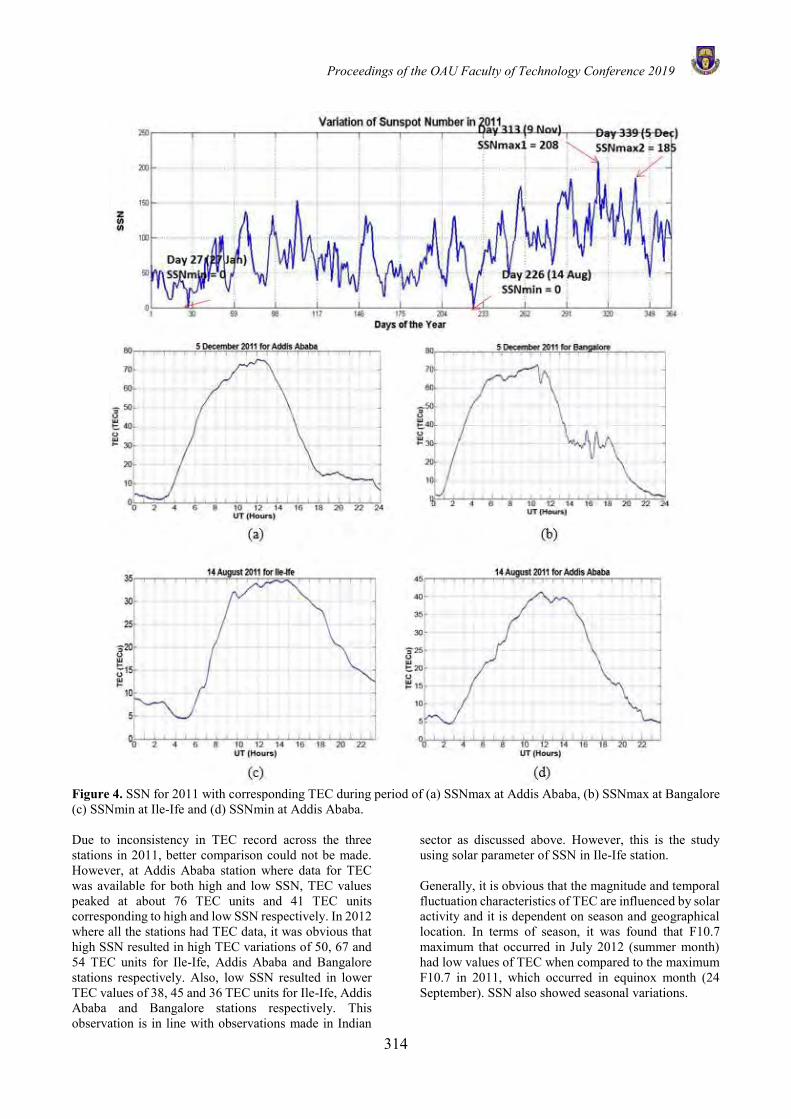
Proceedings of the OAU Faculty of Technology Conference 2019
314
Figure 4. SSN for 2011 with corresponding TEC during period of (a) SSNmax at Addis Ababa, (b) SSNmax at Bangalore (c) SSNmin at Ile-Ife and (d) SSNmin at Addis Ababa. Due to inconsistency in TEC record across the three stations in 2011, better comparison could not be made. However, at Addis Ababa station where data for TEC was available for both high and low SSN, TEC values peaked at about 76 TEC units and 41 TEC units corresponding to high and low SSN respectively. In 2012 where all the stations had TEC data, it was obvious that high SSN resulted in high TEC variations of 50, 67 and 54 TEC units for Ile-Ife, Addis Ababa and Bangalore stations respectively. Also, low SSN resulted in lower TEC values of 38, 45 and 36 TEC units for Ile-Ife, Addis Ababa and Bangalore stations respectively. This observation is in line with observations made in Indian
sector as discussed above. However, this is the study using solar parameter of SSN in Ile-Ife station. Generally, it is obvious that the magnitude and temporal fluctuation characteristics of TEC are influenced by solar activity and it is dependent on season and geographical location. In terms of season, it was found that F10.7 maximum that occurred in July 2012 (summer month) had low values of TEC when compared to the maximum F10.7 in 2011, which occurred in equinox month (24 September). SSN also showed seasonal variations.
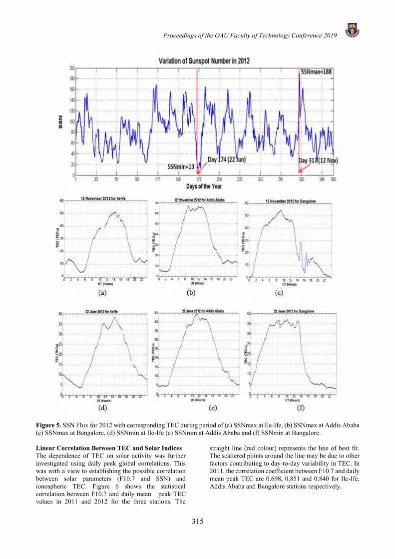
Proceedings of the OAU Faculty of Technology Conference 2019
315
Figure 5. SSN Flux for 2012 with corresponding TEC during period of (a) SSNmax at Ile-Ife, (b) SSNmax at Addis Ababa (c) SSNmax at Bangalore, (d) SSNmin at Ile-Ife (e) SSNmin at Addis Ababa and (f) SSNmin at Bangalore. Linear Correlation Between TEC and Solar Indices The dependence of TEC on solar activity was further investigated using daily peak global correlations. This was with a view to establishing the possible correlation between solar parameters (F10.7 and SSN) and ionospheric TEC. Figure 6 shows the statistical correlation between F10.7 and daily mean peak TEC values in 2011 and 2012 for the three stations. The
straight line (red colour) represents the line of best fit. The scattered points around the line may be due to other factors contributing to day-to-day variability in TEC. In 2011, the correlation coefficient between F10.7 and daily mean peak TEC are 0.698, 0.851 and 0.840 for Ile-Ife, Addis Ababa and Bangalore stations respectively.
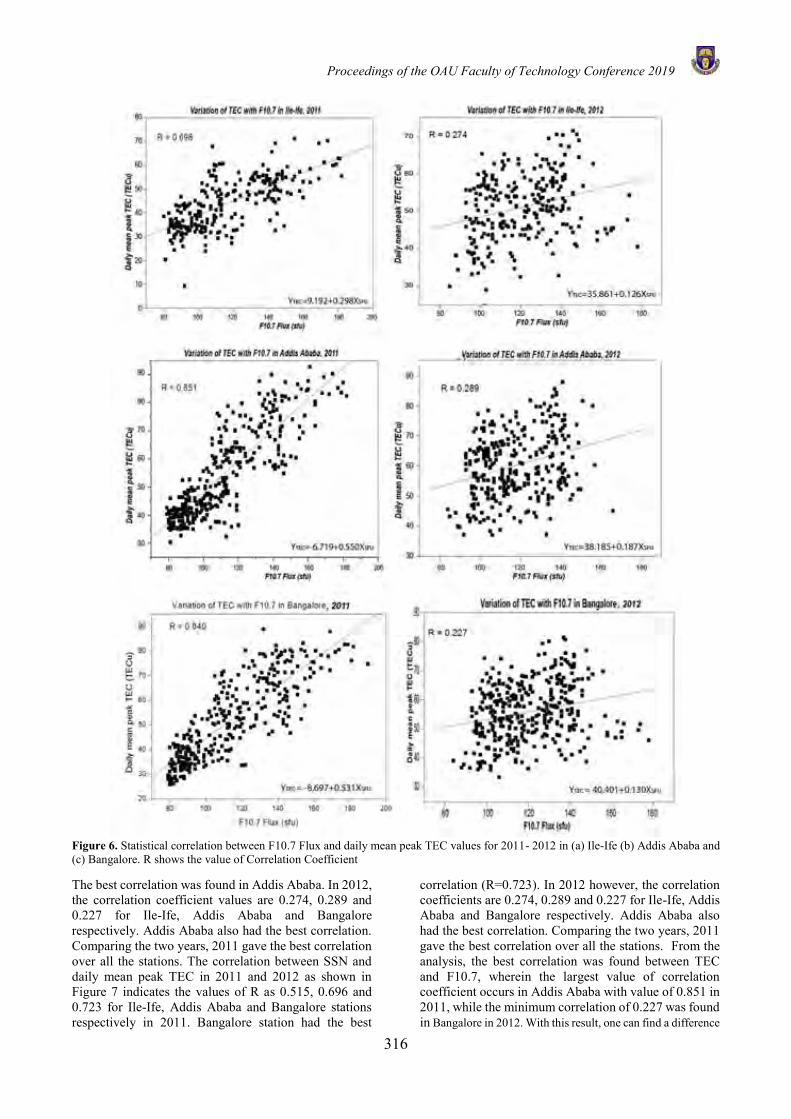
Proceedings of the OAU Faculty of Technology Conference 2019
316
Figure 6. Statistical correlation between F10.7 Flux and daily mean peak TEC values for 2011- 2012 in (a) Ile-Ife (b) Addis Ababa and (c) Bangalore. R shows the value of Correlation Coefficient The best correlation was found in Addis Ababa. In 2012, the correlation coefficient values are 0.274, 0.289 and 0.227 for Ile-Ife, Addis Ababa and Bangalore respectively. Addis Ababa also had the best correlation. Comparing the two years, 2011 gave the best correlation over all the stations. The correlation between SSN and daily mean peak TEC in 2011 and 2012 as shown in Figure 7 indicates the values of R as 0.515, 0.696 and 0.723 for Ile-Ife, Addis Ababa and Bangalore stations respectively in 2011. Bangalore station had the best
correlation (R=0.723). In 2012 however, the correlation coefficients are 0.274, 0.289 and 0.227 for Ile-Ife, Addis Ababa and Bangalore respectively. Addis Ababa also had the best correlation. Comparing the two years, 2011 gave the best correlation over all the stations. From the analysis, the best correlation was found between TEC and F10.7, wherein the largest value of correlation coefficient occurs in Addis Ababa with value of 0.851 in 2011, while the minimum correlation of 0.227 was found in Bangalore in 2012. With this result, one can find a difference
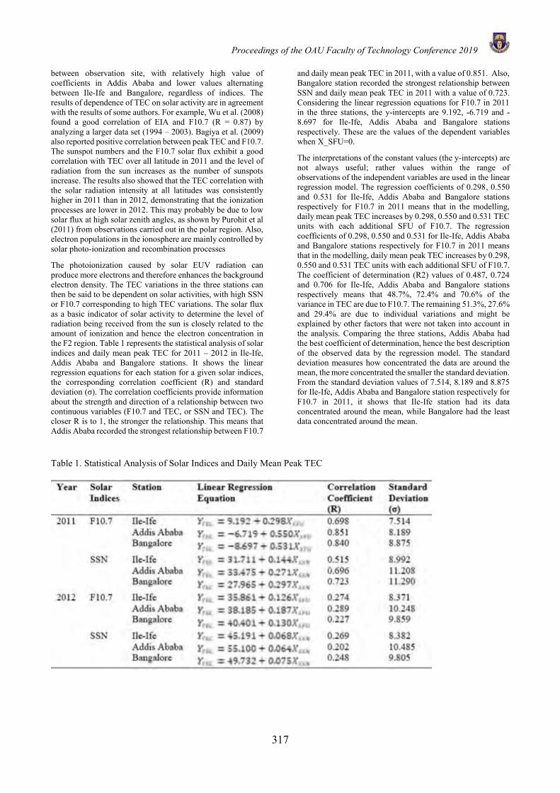
Proceedings of the OAU Faculty of Technology Conference 2019
317
between observation site, with relatively high value of coefficients in Addis Ababa and lower values alternating between Ile-Ife and Bangalore, regardless of indices. The results of dependence of TEC on solar activity are in agreement with the results of some authors. For example, Wu et al. (2008) found a good correlation of EIA and F10.7 (R = 0.87) by analyzing a larger data set (1994 – 2003). Bagiya et al. (2009) also reported positive correlation between peak TEC and F10.7. The sunspot numbers and the F10.7 solar flux exhibit a good correlation with TEC over all latitude in 2011 and the level of radiation from the sun increases as the number of sunspots increase. The results also showed that the TEC correlation with the solar radiation intensity at all latitudes was consistently higher in 2011 than in 2012, demonstrating that the ionization processes are lower in 2012. This may probably be due to low solar flux at high solar zenith angles, as shown by Purohit et al (2011) from observations carried out in the polar region. Also, electron populations in the ionosphere are mainly controlled by solar photo-ionization and recombination processes The photoionization caused by solar EUV radiation can produce more electrons and therefore enhances the background electron density. The TEC variations in the three stations can then be said to be dependent on solar activities, with high SSN or F10.7 corresponding to high TEC variations. The solar flux as a basic indicator of solar activity to determine the level of radiation being received from the sun is closely related to the amount of ionization and hence the electron concentration in the F2 region. Table 1 represents the statistical analysis of solar indices and daily mean peak TEC for 2011 – 2012 in Ile-Ife, Addis Ababa and Bangalore stations. It shows the linear regression equations for each station for a given solar indices, the corresponding correlation coefficient (R) and standard deviation (σ). The correlation coefficients provide information about the strength and direction of a relationship between two continuous variables (F10.7 and TEC, or SSN and TEC). The closer R is to 1, the stronger the relationship. This means that Addis Ababa recorded the strongest relationship between F10.7
and daily mean peak TEC in 2011, with a value of 0.851. Also, Bangalore station recorded the strongest relationship between SSN and daily mean peak TEC in 2011 with a value of 0.723. Considering the linear regression equations for F10.7 in 2011 in the three stations, the y-intercepts are 9.192, -6.719 and -8.697 for Ile-Ife, Addis Ababa and Bangalore stations respectively. These are the values of the dependent variables when X_SFU=0. The interpretations of the constant values (the y-intercepts) are not always useful; rather values within the range of observations of the independent variables are used in the linear regression model. The regression coefficients of 0.298, 0.550 and 0.531 for Ile-Ife, Addis Ababa and Bangalore stations respectively for F10.7 in 2011 means that in the modelling, daily mean peak TEC increases by 0.298, 0.550 and 0.531 TEC units with each additional SFU of F10.7. The regression coefficients of 0.298, 0.550 and 0.531 for Ile-Ife, Addis Ababa and Bangalore stations respectively for F10.7 in 2011 means that in the modelling, daily mean peak TEC increases by 0.298, 0.550 and 0.531 TEC units with each additional SFU of F10.7. The coefficient of determination (R2) values of 0.487, 0.724 and 0.706 for Ile-Ife, Addis Ababa and Bangalore stations respectively means that 48.7%, 72.4% and 70.6% of the variance in TEC are due to F10.7. The remaining 51.3%, 27.6% and 29.4% are due to individual variations and might be explained by other factors that were not taken into account in the analysis. Comparing the three stations, Addis Ababa had the best coefficient of determination, hence the best description of the observed data by the regression model. The standard deviation measures how concentrated the data are around the mean, the more concentrated the smaller the standard deviation. From the standard deviation values of 7.514, 8.189 and 8.875 for Ile-Ife, Addis Ababa and Bangalore station respectively for F10.7 in 2011, it shows that Ile-Ife station had its data concentrated around the mean, while Bangalore had the least data concentrated around the mean.
Table 1. Statistical Analysis of Solar Indices and Daily Mean Peak TEC
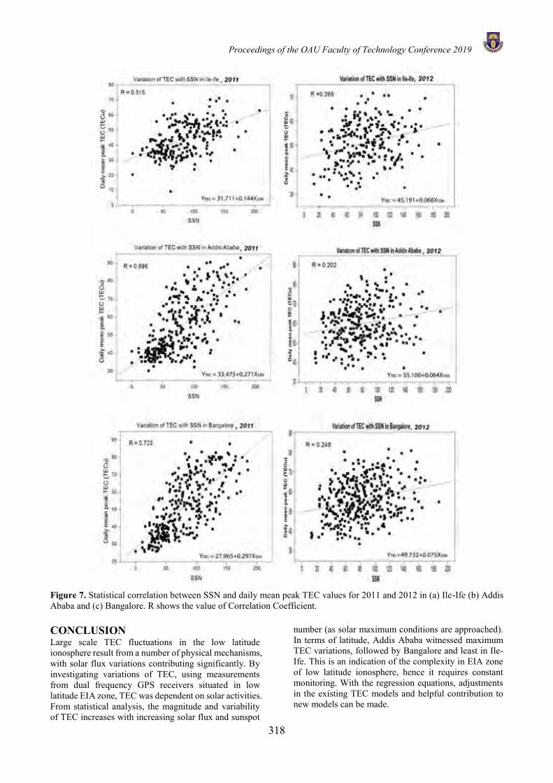
Proceedings of the OAU Faculty of Technology Conference 2019
318
Figure 7. Statistical correlation between SSN and daily mean peak TEC values for 2011 and 2012 in (a) Ile-Ife (b) Addis Ababa and (c) Bangalore. R shows the value of Correlation Coefficient. CONCLUSION Large scale TEC fluctuations in the low latitude ionosphere result from a number of physical mechanisms, with solar flux variations contributing significantly. By investigating variations of TEC, using measurements from dual frequency GPS receivers situated in low latitude EIA zone, TEC was dependent on solar activities. From statistical analysis, the magnitude and variability of TEC increases with increasing solar flux and sunspot
number (as solar maximum conditions are approached). In terms of latitude, Addis Ababa witnessed maximum TEC variations, followed by Bangalore and least in Ile-Ife. This is an indication of the complexity in EIA zone of low latitude ionosphere, hence it requires constant monitoring. With the regression equations, adjustments in the existing TEC models and helpful contribution to new models can be made.
Proceedings of the OAU Faculty of Technology Conference 2019
319
REFERENCES Abdu, M. A., Equatorial ionosphere–thermosphere
system: electrodynamics and irregularities, Adv. Space Res., 35:771–787, 2005.
Bagiya, M. S., Joshi, H. P., Iyer, K. N., Aggarwal, M., Ravindran, S. and Pathan, B. M., TEC variations during low solar activity period (2005 – 2007) near the Equatorial Ionospheric Anomaly Crest region, in India. Annales Geophysicae, 27:1047–1057, 2009.
Bolaji, O. S., Izang P. A., Oladosu, O. R., Koya, F., Fayose, R. S. and Rabiu, A. B., Ionospheric Time-delay over Akure Using Global Positioning System Observations. Acta Geophysica, 63(3):884–899, 2015
Ciraolo, L., Azpilicueta, F., Brunini, C., Meza, A. and Radicella, S. M., Calibration errors on experimental slant total electron content (TEC) determined with GPS. Journal of Geodesy 81(2):111–120, 2007.
Klobuchar, J. A. Ionospheric Effects on GPS, In: Global Positioning System: Theory and Applications, Vol. 1, Parkinson, B. W. & Spilker, J. J. (Eds.), pp 485–515, American Institute of Aeronautic & Astronautics, 1996.
Klobuchar, J., Design and characteristics of the GPS ionospheric time-delay algorithm for single frequency users, in: Proceedings of PLANS’86 –Position Location & Navigation Symposium, Las Vegas, Nevada, 280–286, 4–7, 1986.
Klobuchar, J. A., Ionospheric Effects on GPS. Early Innovation columns, GPS World, 1991.
Olatunbosun, L. G. and Ariyibi, E. A., Studies of Total Electron Content variations at low-latitude stations within the EIA zone. IOSR Journal of Applied Physics, 7(5):12–24, 2015.
Purohit, P. K., Bhawre, P., Mansoori, A. A., Khan, P. A. and Gwal, A. K., GPS derived total electron content (TEC) variations over Indian Antarctic Station, Maitri, World Acad. Sci. Engin. Technol., 59:597-599, 2011.
Sardon, E., Rius, A. and Zarraoa, N., Estimation of the transmitter and receiver differential biases and the ionospheric TEC from GPS observations, Radio Sci., 29:577–586, 1994.
Svalgaard, L. and Hudson, H. S., The Solar Microwave Flux and the Sunspot Number, SOHO-23: Understanding a Peculiar Solar Minimum ASP Conference, 428:325-328, 2010
Wu, C. C., Fry, C. D., Liou, K., Shan, S., and Tseng, C. L., Variation of ionospheric TEC in Taiwan region of the equatorial anomaly from 1994 to 2003. Adv. Space Res., 41:611–616, 2008.
Yizengaw, E., Essex, E. A. and Birsa, R., The Southern Hemisphere and equatorial region ionization response for a 22 September 1999 severe magnetic storm. Ann. Geophys., 22:2765–2773, 2004.
Proceedings of the OAU Faculty of Technology Conference 2019
320
THE SUCTION CONTROL CHARACTERISTICS OF FLOW SEPARATION ON NACA 23012
M. O. Julius1, S. A. Adio*1, A. O. Muritala1 and O. I. Alonge2 1 Department of Mechanical Engineering, Obafemi Awolowo University, Ile-Ife, Osun State, Nigeria.
2 Department of Mechanical Engineering, Elizade University, Ilaramokin, Ondo State, Nigeria.
* Email of Corresponding Author: [email protected]
ABSTRACT The enormous loss of momentum leads to stall and adversely affects the aerodynamic performance of aeroplane wings which may lead to a disaster and put the safety of the aeroplane and the lives on it in danger. Therefore, this paper focuses on the enhancement of aerodynamic characteristics of NACA 23012 through the mitigation of flow separation and delay of the stall at higher angles of attack (10o ≤ α ≥=18o) by using suction for Reynolds number (𝑅𝑒) = 3.4 × 10⁶ . Considering the different suction features such as suction width, suction position, and suction coefficient, the separation delay capability of a suction control is studied. Also, the lift to drag ratio and the impact of energy consumption variation during the control technique are used for estimating the control effects. The Reynolds Average Navier-Stokes (RANS) equations are employed together with the Menter’s shear stress turbulent model. The result of this study revealed that the jet position just behind the separation point at 0.2 % of the chord length shows an outstanding control outcome on the separation and stall, thereby increasing the lift. The lift to drag ration increased proportionately when the suction jet coefficient was increased. At suction coefficients 𝐶𝑞 = 0.00225, a 92.1% drag reduction and 72.7% lift enhancement is observed. Hence, the stall angle is moved beyond 21.5o from an initial angle of 16° and the more energy was saved at a high angle of attack. Keywords: Flow control, aerofoil, lift to drag ratio, suction and boundary layer separation INTRODUCTION The combined effect of adverse pressure gradient and skin friction occur more often at higher angle of attack or low Reynolds numbers, and this will induce enormous energy loss which results to the drop in the aerodynamic performances of aeroplanes during departure, landing and during manoeuvring of unmanned aerial vehicles (UAV) leading to large loss of momentum over the aerofoil. Therefore, many approaches have been deployed to stem the occurrence of these adverse situations in order to promote flow reattachment, thus enhancing aerodynamic performance of the aircraft. Such methods could either be an active method which involves energy expenditure or passive method which does not involve energy spending. Over the past decades, suction control, which is an active technique, is one of the promising means which have been explored. Various scholars have considered different experimental and/or numerical technique to control flow on common NACA aerofoils in order to impede flow transition, enhance lift, postpone separation, reduce drag, suppress noise, and augment turbulence. Although Jacobs and Clay (1936) concluded that NACA 23012 has very good aerodynamic characteristics when compared to Clark y and other types of aerofoils, NACA 23013 is not one of the previously considered aerofoil using suction control technique. Alrefai and Acharya (1996), Karim and Acharyat (1994) experimentally worked on the suction control of dynamic stall vortex of NACA 0012 at Reynolds number between Re = 3.0 × 10⁴ and Re = 1.18 × 10⁵, and suction slot
positioned between 2-5 % of the chord length. There result showed a complete mitigation of flow separation and dynamic stall over a well-defined area of parameter space. Owens and Perkins (1996) experimentally worked on the control of separation of the boundary layer on highly swept cranked delta wing via suction. There results showed an increment in the lift to drag ratio to be 21% plus there was an effective enhancement of the aerodynamic characteristic of the wing. Wahidi and Bridges (2012) experimentally used suction techniques to restrain the size of the laminar separation bubble on LA2573a aerofoil. The suction technique effectively reduced the laminar bubble size and delayed the flow separation cum transition. They achieved 14–24% drag reduction and concluded that the consequence of using suction to reduce the drag is negligible. Chen et al. (2013) experimentally worked on the suppression of vortex shedding on a cylinder using suction flow control technique. They concluded that the suction flow control on the circular cylinder diminished the alternate shedding of the vortex. Additionally, the instabilities in the coefficient of lift and drag of the cylinder were reduced drastically. Atik and Walker (2005) investigated the impact of suction and suction/blowing as control mechanisms for separation that occur at the leading edge at high Reynolds number through a series of numerical simulation. They revealed that the suppression impact of a single suction control technique is better than the blow/suction control technique. Yousefi and Saleh (2015) and Yousefi et al. (2013a), (2014b) worked on the numerical optimization
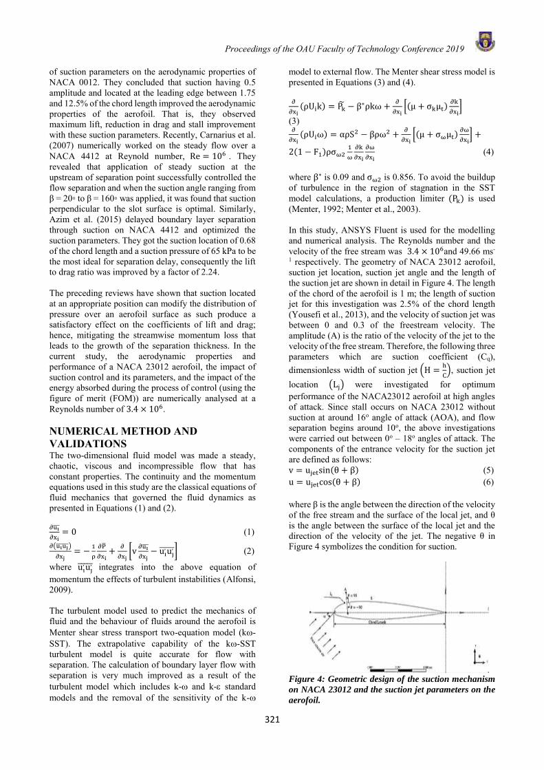
Proceedings of the OAU Faculty of Technology Conference 2019
321
of suction parameters on the aerodynamic properties of NACA 0012. They concluded that suction having 0.5 amplitude and located at the leading edge between 1.75 and 12.5% of the chord length improved the aerodynamic properties of the aerofoil. That is, they observed maximum lift, reduction in drag and stall improvement with these suction parameters. Recently, Carnarius et al. (2007) numerically worked on the steady flow over a NACA 4412 at Reynold number, Re = 106 . They revealed that application of steady suction at the upstream of separation point successfully controlled the flow separation and when the suction angle ranging from β = 20 to β = 160 was applied, it was found that suction perpendicular to the slot surface is optimal. Similarly, Azim et al. (2015) delayed boundary layer separation through suction on NACA 4412 and optimized the suction parameters. They got the suction location of 0.68 of the chord length and a suction pressure of 65 kPa to be the most ideal for separation delay, consequently the lift to drag ratio was improved by a factor of 2.24. The preceding reviews have shown that suction located at an appropriate position can modify the distribution of pressure over an aerofoil surface as such produce a satisfactory effect on the coefficients of lift and drag; hence, mitigating the streamwise momentum loss that leads to the growth of the separation thickness. In the current study, the aerodynamic properties and performance of a NACA 23012 aerofoil, the impact of suction control and its parameters, and the impact of the energy absorbed during the process of control (using the figure of merit (FOM)) are numerically analysed at a Reynolds number of 3.4 × 10⁶. NUMERICAL METHOD AND VALIDATIONS The two-dimensional fluid model was made a steady, chaotic, viscous and incompressible flow that has constant properties. The continuity and the momentum equations used in this study are the classical equations of fluid mechanics that governed the fluid dynamics as presented in Equations (1) and (2). ∂ui
∂xi= 0 (1)
∂(ui uj )
∂xj= −
1
ρ
∂P
∂xi+
∂
∂xj[v
∂ui
∂xj− ui
,uj, ] (2)
where ui,uj
, integrates into the above equation of momentum the effects of turbulent instabilities (Alfonsi, 2009). The turbulent model used to predict the mechanics of fluid and the behaviour of fluids around the aerofoil is Menter shear stress transport two-equation model (k-SST). The extrapolative capability of the k-SST turbulent model is quite accurate for flow with separation. The calculation of boundary layer flow with separation is very much improved as a result of the turbulent model which includes k- and k- standard models and the removal of the sensitivity of the k-
model to external flow. The Menter shear stress model is presented in Equations (3) and (4). ∂
∂xi(ρUik) = Pk − β∗ρkω +
∂
∂xi[(μ + σkμt)
∂k
∂xi]
(3) ∂
∂xi(ρUiω) = αρS2 − βρω2 +
∂
∂xi[(μ + σωμt)
∂ω
∂xi] +
2(1 − F1)ρσω21
ω
∂k
∂xi
∂ω
∂xi (4)
where β∗ is 0.09 and σω2 is 0.856. To avoid the buildup of turbulence in the region of stagnation in the SST model calculations, a production limiter (Pk) is used (Menter, 1992; Menter et al., 2003). In this study, ANSYS Fluent is used for the modelling and numerical analysis. The Reynolds number and the velocity of the free stream was 3.4 × 10⁶and 49.66 ms-
1 respectively. The geometry of NACA 23012 aerofoil, suction jet location, suction jet angle and the length of the suction jet are shown in detail in Figure 4. The length of the chord of the aerofoil is 1 m; the length of suction jet for this investigation was 2.5% of the chord length (Yousefi et al., 2013), and the velocity of suction jet was between 0 and 0.3 of the freestream velocity. The amplitude (A) is the ratio of the velocity of the jet to the velocity of the free stream. Therefore, the following three parameters which are suction coefficient (Cq), dimensionless width of suction jet (H =
h
C), suction jet
location (Lj) were investigated for optimum performance of the NACA23012 aerofoil at high angles of attack. Since stall occurs on NACA 23012 without suction at around 16o angle of attack (AOA), and flow separation begins around 10o, the above investigations were carried out between 0o – 18o angles of attack. The components of the entrance velocity for the suction jet are defined as follows: v = ujetsin(θ + β) (5) u = ujetcos(θ + β) (6) where β is the angle between the direction of the velocity of the free stream and the surface of the local jet, and θ is the angle between the surface of the local jet and the direction of the velocity of the jet. The negative θ in Figure 4 symbolizes the condition for suction.
Figure 4: Geometric design of the suction mechanism
on NACA 23012 and the suction jet parameters on the
aerofoil.
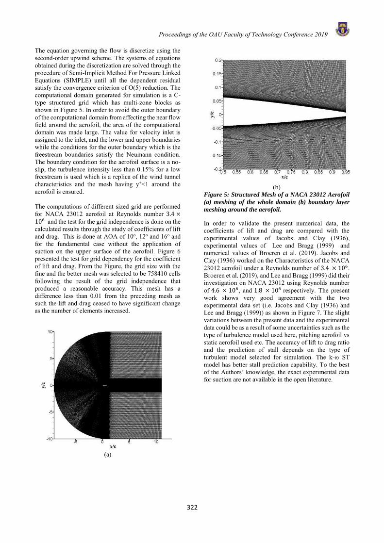
Proceedings of the OAU Faculty of Technology Conference 2019
322
The equation governing the flow is discretize using the second-order upwind scheme. The systems of equations obtained during the discretization are solved through the procedure of Semi-Implicit Method For Pressure Linked Equations (SIMPLE) until all the dependent residual satisfy the convergence criterion of O(5) reduction. The computational domain generated for simulation is a C-type structured grid which has multi-zone blocks as shown in Figure 5. In order to avoid the outer boundary of the computational domain from affecting the near flow field around the aerofoil, the area of the computational domain was made large. The value for velocity inlet is assigned to the inlet, and the lower and upper boundaries while the conditions for the outer boundary which is the freestream boundaries satisfy the Neumann condition. The boundary condition for the aerofoil surface is a no-slip, the turbulence intensity less than 0.15% for a low freestream is used which is a replica of the wind tunnel characteristics and the mesh having y+<1 around the aerofoil is ensured. The computations of different sized grid are performed for NACA 23012 aerofoil at Reynolds number 3.4 ×10⁶ and the test for the grid independence is done on the calculated results through the study of coefficients of lift and drag. This is done at AOA of 10o, 12o and 16o and for the fundamental case without the application of suction on the upper surface of the aerofoil. Figure 6 presented the test for grid dependency for the coefficient of lift and drag. From the Figure, the grid size with the fine and the better mesh was selected to be 758410 cells following the result of the grid independence that produced a reasonable accuracy. This mesh has a difference less than 0.01 from the preceding mesh as such the lift and drag ceased to have significant change as the number of elements increased.
(a)
(b)
Figure 5: Structured Mesh of a NACA 23012 Aerofoil
(a) meshing of the whole domain (b) boundary layer
meshing around the aerofoil.
In order to validate the present numerical data, the coefficients of lift and drag are compared with the experimental values of Jacobs and Clay (1936), experimental values of Lee and Bragg (1999) and numerical values of Broeren et al. (2019). Jacobs and Clay (1936) worked on the Characteristics of the NACA 23012 aerofoil under a Reynolds number of 3.4 × 10⁶. Broeren et al. (2019), and Lee and Bragg (1999) did their investigation on NACA 23012 using Reynolds number of 4.6 × 10⁶, and 1.8 × 10⁶ respectively. The present work shows very good agreement with the two experimental data set (i.e. Jacobs and Clay (1936) and Lee and Bragg (1999)) as shown in Figure 7. The slight variations between the present data and the experimental data could be as a result of some uncertainties such as the type of turbulence model used here, pitching aerofoil vs static aerofoil used etc. The accuracy of lift to drag ratio and the prediction of stall depends on the type of turbulent model selected for simulation. The k-ω ST model has better stall prediction capability. To the best of the Authors’ knowledge, the exact experimental data for suction are not available in the open literature.
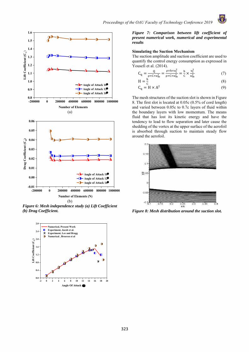
Proceedings of the OAU Faculty of Technology Conference 2019
323
(a)
(b)
Figure 6: Mesh independence study (a) Lift Coefficient
(b) Drag Coefficient.
Figure 7: Comparison between lift coefficient of
present numerical work, numerical and experimental
results
Simulating the Suction Mechanism The suction amplitude and suction coefficient are used to quantify the control energy consumption as expressed in Yousefi et al. (2014).
Cq =Q
ρ×C×u∞2 =
ρ×h×uj2
ρ×C×u∞2 =
h
C×
uj2
u∞2 (7)
H =h
C (8)
Cq = H × A2 (9) The mesh structures of the suction slot is shown in Figure 8. The first slot is located at 0.05c (0.5% of cord length) and varied between 0.05c to 0.7c layers of fluid within the boundary layers with low momentum. The means fluid that has lost its kinetic energy and have the tendency to lead to flow separation and later cause the shedding of the vortex at the upper surface of the aerofoil is absorbed through suction to maintain steady flow around the aerofoil.
Figure 8: Mesh distribution around the suction slot.
-200000 0 200000 400000 600000 800000 10000000.8
0.9
1.0
1.1
1.2
1.3
1.4
1.5
1.6
Lift
Coe
ffic
ient
(CL)
Number of Elements
Angle of Attack 10° Angle of Attack 12° Angle of Attack 16°
-200000 0 200000 400000 600000 800000 1000000-0.01
0.00
0.01
0.02
0.03
0.04
0.05
0.06
Dra
g C
oeff
icie
nt (C
d)
Number of Elements (N)
Angle of Attack 10° Angle of Attack 12° Angle of Attack 16°
-2 0 2 4 6 8 10 12 14 16 18 200.0
0.4
0.8
1.2
1.6
2.0
2.4
2.8
Lift
Coe
ffic
ient
(CL)
Angle Of Attack ()
Numerical, Present Work Experiment, Jacob et al. Experiment, Lee and Bragg Numerical , Broeren et al
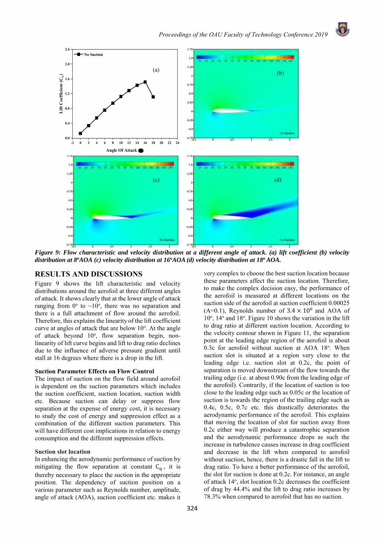
Proceedings of the OAU Faculty of Technology Conference 2019
324
Figure 9: Flow characteristic and velocity distribution at a different angle of attack. (a) lift coefficient (b) velocity
distribution at 8oAOA (c) velocity distribution at 16oAOA (d) velocity distribution at 18o AOA. RESULTS AND DISCUSSIONS Figure 9 shows the lift characteristic and velocity distributions around the aerofoil at three different angles of attack. It shows clearly that at the lower angle of attack ranging from 0o to ~10o, there was no separation and there is a full attachment of flow around the aerofoil. Therefore, this explains the linearity of the lift coefficient curve at angles of attack that are below 10o. At the angle of attack beyond 10o, flow separation begin, non-linearity of lift curve begins and lift to drag ratio declines due to the influence of adverse pressure gradient until stall at 16 degrees where there is a drop in the lift. Suction Parameter Effects on Flow Control The impact of suction on the flow field around aerofoil is dependent on the suction parameters which includes the suction coefficient, suction location, suction width etc. Because suction can delay or suppress flow separation at the expense of energy cost, it is necessary to study the cost of energy and suppression effect as a combination of the different suction parameters. This will have different cost implications in relation to energy consumption and the different suppression effects. Suction slot location In enhancing the aerodynamic performance of suction by mitigating the flow separation at constant Cq , it is thereby necessary to place the suction in the appropriate position. The dependency of suction position on a various parameter such as Reynolds number, amplitude, angle of attack (AOA), suction coefficient etc. makes it
very complex to choose the best suction location because these parameters affect the suction location. Therefore, to make the complex decision easy, the performance of the aerofoil is measured at different locations on the suction side of the aerofoil at suction coefficient 0.00025 (A=0.1), Reynolds number of 3.4 × 10⁶ and AOA of 10o, 14o and 18o. Figure 10 shows the variation in the lift to drag ratio at different suction location. According to the velocity contour shown in Figure 11, the separation point at the leading edge region of the aerofoil is about 0.3c for aerofoil without suction at AOA 18o. When suction slot is situated at a region very close to the leading edge i.e. suction slot at 0.2c, the point of separation is moved downstream of the flow towards the trailing edge (i.e. at about 0.90c from the leading edge of the aerofoil). Contrarily, if the location of suction is too close to the leading edge such as 0.05c or the location of suction is towards the region of the trailing edge such as 0.4c, 0.5c, 0.7c etc. this drastically deteriorates the aerodynamic performance of the aerofoil. This explains that moving the location of slot for suction away from 0.2c either way will produce a catastrophic separation and the aerodynamic performance drops as such the increase in turbulence causes increase in drag coefficient and decrease in the lift when compared to aerofoil without suction, hence, there is a drastic fall in the lift to drag ratio. To have a better performance of the aerofoil, the slot for suction is done at 0.2c. For instance, an angle of attack 14o, slot location 0.2c decreases the coefficient of drag by 44.4% and the lift to drag ratio increases by 78.3% when compared to aerofoil that has no suction.
-2 0 2 4 6 8 10 12 14 16 18 20 22 240.0
0.4
0.8
1.2
1.6
2.0
2.4
Lift
Coe
ffic
ient
(CL)
Angle Of Attack ()
No Suction
(a) (b)
(c) (d)
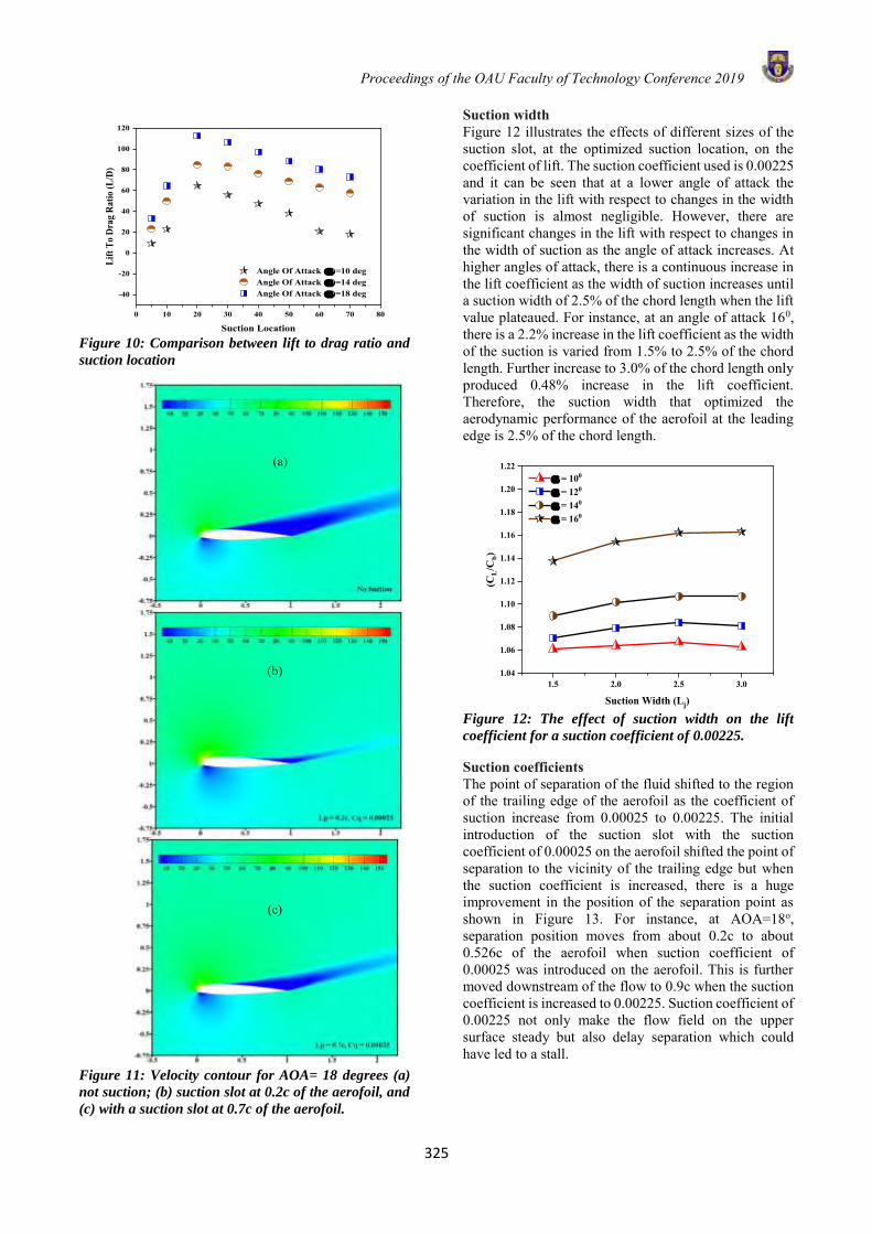
Proceedings of the OAU Faculty of Technology Conference 2019
325
Figure 10: Comparison between lift to drag ratio and
suction location
Figure 11: Velocity contour for AOA= 18 degrees (a)
not suction; (b) suction slot at 0.2c of the aerofoil, and
(c) with a suction slot at 0.7c of the aerofoil.
Suction width Figure 12 illustrates the effects of different sizes of the suction slot, at the optimized suction location, on the coefficient of lift. The suction coefficient used is 0.00225 and it can be seen that at a lower angle of attack the variation in the lift with respect to changes in the width of suction is almost negligible. However, there are significant changes in the lift with respect to changes in the width of suction as the angle of attack increases. At higher angles of attack, there is a continuous increase in the lift coefficient as the width of suction increases until a suction width of 2.5% of the chord length when the lift value plateaued. For instance, at an angle of attack 160, there is a 2.2% increase in the lift coefficient as the width of the suction is varied from 1.5% to 2.5% of the chord length. Further increase to 3.0% of the chord length only produced 0.48% increase in the lift coefficient. Therefore, the suction width that optimized the aerodynamic performance of the aerofoil at the leading edge is 2.5% of the chord length.
Figure 12: The effect of suction width on the lift
coefficient for a suction coefficient of 0.00225.
Suction coefficients The point of separation of the fluid shifted to the region of the trailing edge of the aerofoil as the coefficient of suction increase from 0.00025 to 0.00225. The initial introduction of the suction slot with the suction coefficient of 0.00025 on the aerofoil shifted the point of separation to the vicinity of the trailing edge but when the suction coefficient is increased, there is a huge improvement in the position of the separation point as shown in Figure 13. For instance, at AOA=18o, separation position moves from about 0.2c to about 0.526c of the aerofoil when suction coefficient of 0.00025 was introduced on the aerofoil. This is further moved downstream of the flow to 0.9c when the suction coefficient is increased to 0.00225. Suction coefficient of 0.00225 not only make the flow field on the upper surface steady but also delay separation which could have led to a stall.
0 10 20 30 40 50 60 70 80
-40
-20
0
20
40
60
80
100
120
Lift
To D
rag
Ratio
(L/D
)
Suction Location
Angle Of Attack ()=10 deg Angle Of Attack ()=14 deg Angle Of Attack ()=18 deg
1.5 2.0 2.5 3.01.04
1.06
1.08
1.10
1.12
1.14
1.16
1.18
1.20
1.22 = 100
= 120
= 140
= 160
(CL/C
b)
Suction Width (Lj)
(a)
(b)
(c)
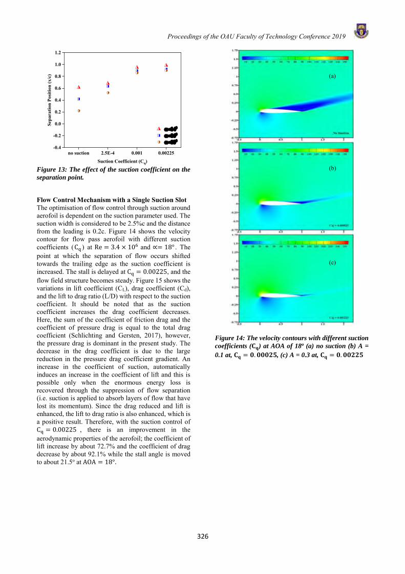
Proceedings of the OAU Faculty of Technology Conference 2019
326
Figure 13: The effect of the suction coefficient on the
separation point.
Flow Control Mechanism with a Single Suction Slot The optimisation of flow control through suction around aerofoil is dependent on the suction parameter used. The suction width is considered to be 2.5%c and the distance from the leading is 0.2c. Figure 14 shows the velocity contour for flow pass aerofoil with different suction coefficients (Cq ) at Re = 3.4 × 10⁶ and ∝= 18° . The point at which the separation of flow occurs shifted towards the trailing edge as the suction coefficient is increased. The stall is delayed at Cq = 0.00225, and the flow field structure becomes steady. Figure 15 shows the variations in lift coefficient (CL), drag coefficient (Cd), and the lift to drag ratio (L/D) with respect to the suction coefficient. It should be noted that as the suction coefficient increases the drag coefficient decreases. Here, the sum of the coefficient of friction drag and the coefficient of pressure drag is equal to the total drag coefficient (Schlichting and Gersten, 2017), however, the pressure drag is dominant in the present study. The decrease in the drag coefficient is due to the large reduction in the pressure drag coefficient gradient. An increase in the coefficient of suction, automatically induces an increase in the coefficient of lift and this is possible only when the enormous energy loss is recovered through the suppression of flow separation (i.e. suction is applied to absorb layers of flow that have lost its momentum). Since the drag reduced and lift is enhanced, the lift to drag ratio is also enhanced, which is a positive result. Therefore, with the suction control of Cq = 0.00225 , there is an improvement in the aerodynamic properties of the aerofoil; the coefficient of lift increase by about 72.7% and the coefficient of drag decrease by about 92.1% while the stall angle is moved to about 21.5o at AOA = 18°.
Figure 14: The velocity contours with different suction
coefficients (𝐂𝐪) at AOA of 18o (a) no suction (b) A =
0.1 at, 𝐂𝐪 = 𝟎. 𝟎𝟎𝟎𝟐𝟓, (c) A = 0.3 at, 𝐂𝐪 = 𝟎. 𝟎𝟎𝟐𝟐𝟓
no suction 2.5E-4 0.001 0.00225-0.4
-0.2
0.0
0.2
0.4
0.6
0.8
1.0
1.2Se
para
tion
Posi
tion
(x/c
)
Suction Coefficient (Cq)
=140
=160
=180
(a)
(b)
(c)
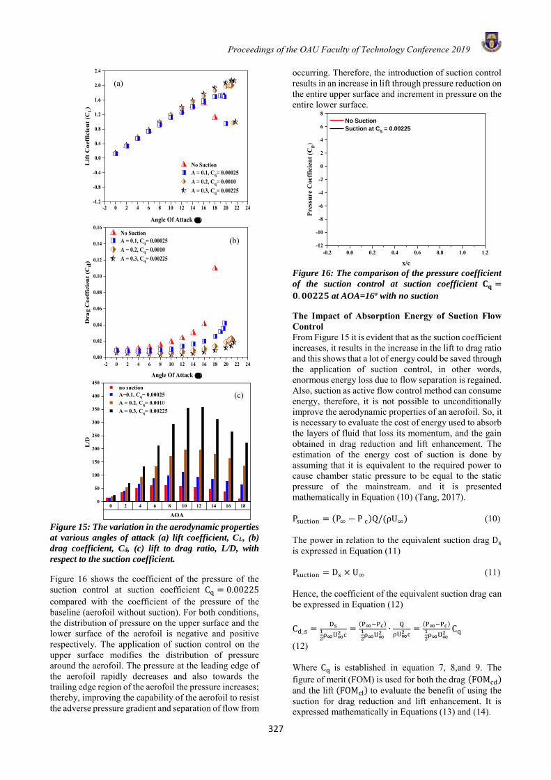
Proceedings of the OAU Faculty of Technology Conference 2019
327
Figure 15: The variation in the aerodynamic properties
at various angles of attack (a) lift coefficient, CL, (b)
drag coefficient, Cd, (c) lift to drag ratio, L/D, with
respect to the suction coefficient.
Figure 16 shows the coefficient of the pressure of the suction control at suction coefficient Cq = 0.00225 compared with the coefficient of the pressure of the baseline (aerofoil without suction). For both conditions, the distribution of pressure on the upper surface and the lower surface of the aerofoil is negative and positive respectively. The application of suction control on the upper surface modifies the distribution of pressure around the aerofoil. The pressure at the leading edge of the aerofoil rapidly decreases and also towards the trailing edge region of the aerofoil the pressure increases; thereby, improving the capability of the aerofoil to resist the adverse pressure gradient and separation of flow from
occurring. Therefore, the introduction of suction control results in an increase in lift through pressure reduction on the entire upper surface and increment in pressure on the entire lower surface.
Figure 16: The comparison of the pressure coefficient
of the suction control at suction coefficient 𝐂𝐪 =
𝟎. 𝟎𝟎𝟐𝟐𝟓 at AOA=16o with no suction
The Impact of Absorption Energy of Suction Flow Control From Figure 15 it is evident that as the suction coefficient increases, it results in the increase in the lift to drag ratio and this shows that a lot of energy could be saved through the application of suction control, in other words, enormous energy loss due to flow separation is regained. Also, suction as active flow control method can consume energy, therefore, it is not possible to unconditionally improve the aerodynamic properties of an aerofoil. So, it is necessary to evaluate the cost of energy used to absorb the layers of fluid that loss its momentum, and the gain obtained in drag reduction and lift enhancement. The estimation of the energy cost of suction is done by assuming that it is equivalent to the required power to cause chamber static pressure to be equal to the static pressure of the mainstream. and it is presented mathematically in Equation (10) (Tang, 2017). Psuction = (P∞ − P c)Q/(ρU∞) (10) The power in relation to the equivalent suction drag Ds is expressed in Equation (11) Psuction = Ds × U∞ (11) Hence, the coefficient of the equivalent suction drag can be expressed in Equation (12) Cd_s =
Ds1
2ρ∞U∞
2 c=
(P∞−Pc)1
2ρ∞U∞
2∙
Q
ρU∞2 c
=(P∞−Pc)1
2ρ∞U∞
2Cq
(12) Where Cq is established in equation 7, 8,and 9. The figure of merit (FOM) is used for both the drag (FOMcd) and the lift (FOMcl) to evaluate the benefit of using the suction for drag reduction and lift enhancement. It is expressed mathematically in Equations (13) and (14).
-0.2 0.0 0.2 0.4 0.6 0.8 1.0 1.2-12
-10
-8
-6
-4
-2
0
2
4
6
8 No Suction
Suction at Cq = 0.00225
Pres
sure
Coe
ffic
ient
(Cp)
x/c
-2 0 2 4 6 8 10 12 14 16 18 20 22 24-1.2
-0.8
-0.4
0.0
0.4
0.8
1.2
1.6
2.0
2.4
Lif
t Coe
ffic
ient
(CL)
Angle Of Attack ()
No Suction A = 0.1, Cq= 0.00025 A = 0.2, Cq= 0.0010 A = 0.3, Cq= 0.00225
-2 0 2 4 6 8 10 12 14 16 18 20 22 240.00
0.02
0.04
0.06
0.08
0.10
0.12
0.14
0.16
Dra
g C
oeff
icie
nt (C
d)
Angle Of Attack ()
No Suction A = 0.1, Cq= 0.00025 A = 0.2, Cq= 0.0010 A = 0.3, Cq= 0.00225
0 2 4 6 8 10 12 14 16 18
AOA
0
50
100
150
200
250
300
350
400
450
L/D
no suction A=0.1, Cq= 0.00025 A = 0.2, Cq= 0.0010 A = 0.3, Cq= 0.00225
(a)
(b)
(c)
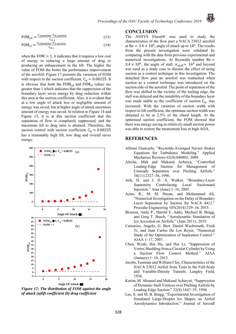
Proceedings of the OAU Faculty of Technology Conference 2019
328
FOMcd =
C_baseline−Cd_suction
Cd_s (13)
FOMcl =Cl_baseline−Cl_suction
Cd_s (14)
when the FOM > 1, it indicates that it requires a low cost of energy to reducing a large amount of drag or producing an enhancement in the lift. The higher the value of FOM the better the performance improvement of the aerofoil. Figure 17 presents the variation of FOM with respect to the suction coefficient, Cq = 0.00225. It is obvious that both the FOMcd and FOMcl values are greater than 1 which indicates that the suppression of the boundary layer saves energy by drag reduction within this area at the suction coefficient. Also, it is evident that at a low angle of attack less or negligible amount of energy was saved, but at higher angle of attack enormous amount of energy was saved. In relation to Figure 14 and Figure 15, it is at this suction coefficient that the separation of flow is completely suppressed, and the maximum lift to drag ratio is attained. Therefore, the suction control with suction coefficient, Cq = 0.00225 has a reasonably high lift, low drag and overall saves energy.
Figure 17: The distribution of FOM against the angle
of attack (a)lift coefficient (b) drag coefficient
CONCLUSION The ANSYS Fluent® was used to study the characteristics of the flow past a NACA 23012 aerofoil at Re = 3.4 × 10⁶, angle of attack up to 18°. The results from the present investigation were validated by comparing with the data from previous experimental and numerical investigations. At Reynolds number Re =3.4 × 10⁶ , the angle of stall, ∝stall= 160 and beyond was used as a study case to discuss the effect of using suction as a control technique in this investigation. The detached flow past an aerofoil was reattached when suction as a control technique was introduced on the suction side of the aerofoil. The point of separation of the flow was shifted to the vicinity of the trailing edge, the stall was delayed and the instability of the boundary layer was made stable as the coefficient of suction Cq , was increased. With the variation of suction width with respect to lift coefficient, the optimum suction width was obtained to be at 2.5% of the chord length. At the optimised suction coefficient, the FOM showed that there was energy saving as relatively small suction power was able to restore the momentum loss at high AOA. REFERENCES
Alfonsi Giancarlo, “Reynolds-Averaged Navier–Stokes Equations for Turbulence Modeling.” Applied Mechanics Reviews 62(4):040802, 2009.
Alrefai, Mah and Mukund Acharya, “Controlled Leading-Edge Suction for Management of Unsteady Separation over Pitching Airfoils.” 34(11):2327–36, 1996.
Atik, H. and J. D. A. Walker, “Boundary-Layer Separation Controlusing Local Suctionand Injection.” Aiaa (June):1–16, 2005.
Azim, R., M. M. Hasan, and Mohammad Ali, “Numerical Investigation on the Delay of Boundary Layer Separation by Suction for NACA 4412.” Procedia Engineering 105(2014):329–34, 2015.
Broeren, Andy P., Harold E. Addy, Michael B. Bragg, and Greg T. Busch, “Aerodynamic Simulation of Ice Accretion on Airfoils.” (June 2011), 2019.
Carnarius, Angelo, G. Bert, Daniel Wachsmuth, Fredi Tr, and Juan Carlos De Los Reyes, “Numerical Study of the Optimization of Separation Control.” AIAA 1–17, 2007.
Chen, Wenli, Hui Hu, and Hui Li, “Suppression of Vortex Shedding from a Circular Cylinder by Using a Suction Flow Control Method.” AIAA (January):1–10, 2013.
Jacobs, Eastman and William Clay, Characteristics of the NACA 23012 Airfoil from Tests in the Full-Scale and Variable-Density Tunnels. Langley Field, 1936.
Karim, M. Ahsanul and Mukund Acharyat, “Suppression of Dynamic-Stall Vortices over Pitching Airfoils by Leading-Edge Suction.” 32(8):1647–55, 1994.
Lee, S. and M. B. Bragg, “Experimental Investigation of Simulated Large-Droplet Ice Shapes on Airfoil Aerodynamics Introduction.” Journal of Aircraft
0 5 10 15 20-505
10152025303540455055606570
FOMcd 1, Cq = 0.00225 FOM = 1
FOM
cd
Angle Of Attack ()
0 5 10 15 20
0
100
200
300
400
500
600 FOMcl 1, Cq = 0.00225 FOM = 1
FOM
cl
Angle Of Attack ()
(a)
(b)

Proceedings of the OAU Faculty of Technology Conference 2019
329
36(5):844–50, 1999. Menter, F. R., M. Kuntz, and R. Langtry, “Ten Years of
Industrial Experience with the SST Turbulence Model.” Pp. 625–32 in Turbulence Heat and Mass Transfer 4. Vol. 4. Turkey: Heat and Mass Transfer, 2003.
Menter, Florian R, Improved Two-Equation Turbulence Models for Aerodynamic Flows. Moffett Field, 1992.
Owens, D. B. and John N. Perkins, “Improved Performance on Highly Swept Wings by Suction Boundary-Layer Control.” AIAA (January):96, 1996.
Schlichting, Hermann(Deceased) and Klaus Gersten, Boundary- Layer Theory. 9th Editio. Berlin Heidelberg: Springer Nature, 2017.
Tang, Qizhong,“Main Characteristics of Suction Control of Flow Separation of an Airfoil at Low Reynolds Numbers.” European Journal of Mechanics, B/Fluids 65:88–97, 2017.
Wahidi, Redha and David H. Bridges, “Effects of Distributed Suction on an Airfoil.” AIAA JOURNAL 50(3), 2012.
Yousefi, Kianoosh and Reza Saleh, “Three-Dimensional Suction Flow Control and Suction Jet Length Optimization of NACA 0012 Wing.” Meccanica 50(6):1481–94, 2015.
Yousefi, Kianoosh, Reza Saleh, and Peyman Zahedi, “Numerical Study of Blowing and Suction Slot Geometry Optimization on NACA 0012 Airfoil.” Journal of Mechanical Science and Technology 28(4):1297–1310, 2014b.
Yousefi, Kianoosh, S. Reza Saleh, and Peyman Zahedi, “Numerical Investigation of Suction and Length of Suction Jet on Aerodynamic Characteristics of the NACA 0012 Airfoil.” International Journal of Materials, Mechanics and Manufacturing 1(2):136–42, 2013a.
NOMENCLATURE
𝛼 aerofoil angle of attack [degree] x/c separation position [-] 𝑣 the kinematic viscosity [kgm-1s-1] 𝛼𝑠𝑡𝑎𝑙𝑙 angle of attack at stall Re Reynolds number [-] 𝑢𝑗𝑒𝑡 the suction jet velocity [m/s]
c aerofoil chord length [m] 𝐿𝑗 suction width [m] 𝑢∞ the free stream velocity [m/s] 𝐶𝑞 suction coefficient [-] A suction jet amplitude [-] the mean velocity [m/s] H dimensionless jet width [-] 𝐿𝑝 suction position [m] 𝑢𝑖
,𝑢𝑗, the Reynolds stress tensor [-]
𝐶𝑑 drag coefficient [-] 𝜌 the density of the fluid [kg/m3] 𝐹1 the blending function [-] 𝐶𝐿 lift coefficient [-] N number of elements [-] 𝑆 the invariant measure of the strain rate
[kg/m2] AOA the angle of attack [degree] the mean pressure [kPa] 𝑈𝑚𝑎𝑥 maximum velocity [m/s] 𝑈𝑎𝑣𝑒 average velocity [m/s] 𝑃𝑠𝑢𝑐𝑡𝑖𝑜𝑛 suction power [Joules] 𝑃∞ mainstream static pressure [kPa] 𝑃𝑐 local static pressure of the slot [kPa] 𝐷𝑠 equivalent suction drag
[Newton] 𝐶𝑑_𝑠 equivalent suction drag coefficient [-]
𝐶𝑑_𝑏𝑎𝑠𝑒𝑙𝑖𝑛𝑒 drag coefficient without suction [-] 𝐶𝑑_𝑠𝑢𝑐𝑡𝑖𝑜𝑛 drag coefficient with suction [-]
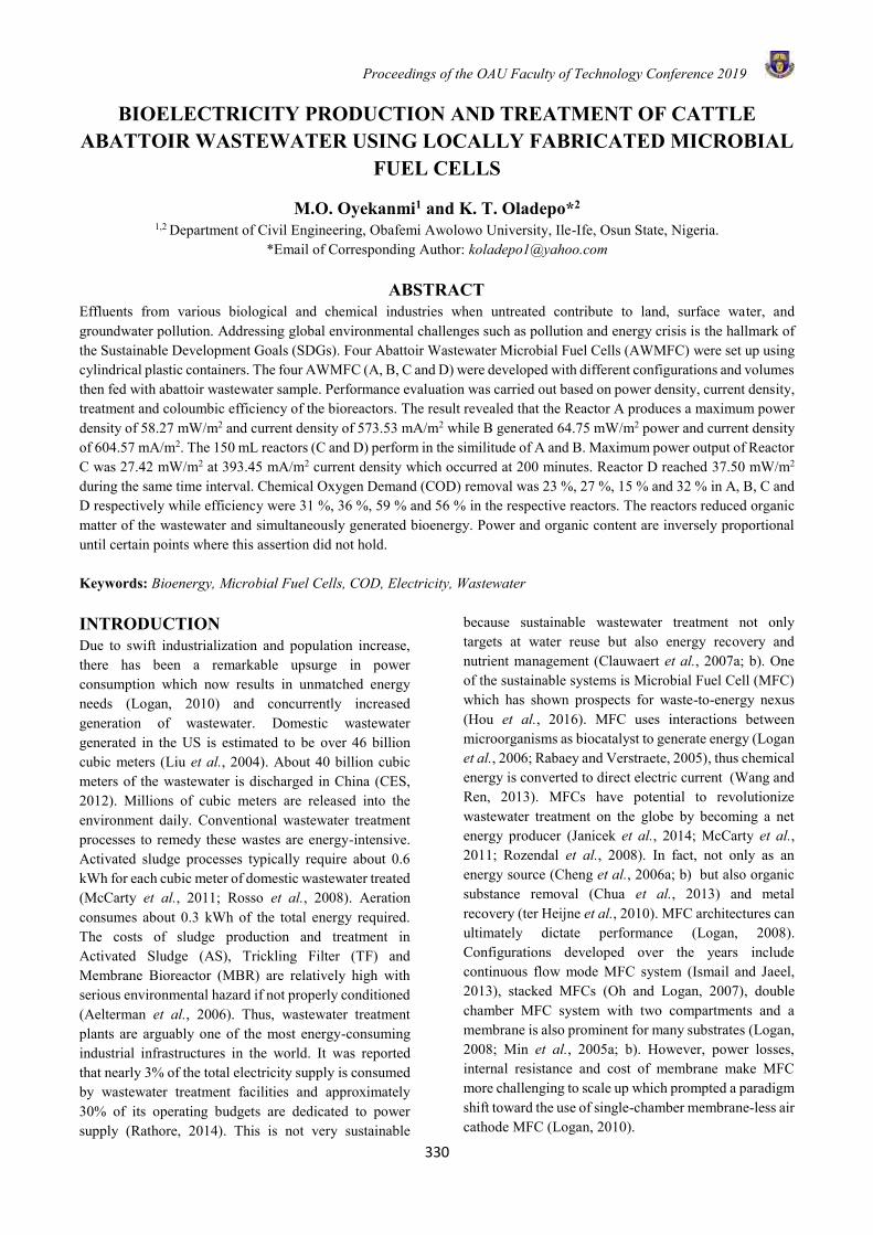
Proceedings of the OAU Faculty of Technology Conference 2019
330
BIOELECTRICITY PRODUCTION AND TREATMENT OF CATTLE ABATTOIR WASTEWATER USING LOCALLY FABRICATED MICROBIAL
FUEL CELLS
M.O. Oyekanmi1 and K. T. Oladepo*2 1,2 Department of Civil Engineering, Obafemi Awolowo University, Ile-Ife, Osun State, Nigeria.
*Email of Corresponding Author: [email protected]
ABSTRACT Effluents from various biological and chemical industries when untreated contribute to land, surface water, and groundwater pollution. Addressing global environmental challenges such as pollution and energy crisis is the hallmark of the Sustainable Development Goals (SDGs). Four Abattoir Wastewater Microbial Fuel Cells (AWMFC) were set up using cylindrical plastic containers. The four AWMFC (A, B, C and D) were developed with different configurations and volumes then fed with abattoir wastewater sample. Performance evaluation was carried out based on power density, current density, treatment and coloumbic efficiency of the bioreactors. The result revealed that the Reactor A produces a maximum power density of 58.27 mW/m2 and current density of 573.53 mA/m2 while B generated 64.75 mW/m2 power and current density of 604.57 mA/m2. The 150 mL reactors (C and D) perform in the similitude of A and B. Maximum power output of Reactor C was 27.42 mW/m2 at 393.45 mA/m2 current density which occurred at 200 minutes. Reactor D reached 37.50 mW/m2 during the same time interval. Chemical Oxygen Demand (COD) removal was 23 %, 27 %, 15 % and 32 % in A, B, C and D respectively while efficiency were 31 %, 36 %, 59 % and 56 % in the respective reactors. The reactors reduced organic matter of the wastewater and simultaneously generated bioenergy. Power and organic content are inversely proportional until certain points where this assertion did not hold. Keywords: Bioenergy, Microbial Fuel Cells, COD, Electricity, Wastewater INTRODUCTION Due to swift industrialization and population increase, there has been a remarkable upsurge in power consumption which now results in unmatched energy needs (Logan, 2010) and concurrently increased generation of wastewater. Domestic wastewater generated in the US is estimated to be over 46 billion cubic meters (Liu et al., 2004). About 40 billion cubic meters of the wastewater is discharged in China (CES, 2012). Millions of cubic meters are released into the environment daily. Conventional wastewater treatment processes to remedy these wastes are energy-intensive. Activated sludge processes typically require about 0.6 kWh for each cubic meter of domestic wastewater treated (McCarty et al., 2011; Rosso et al., 2008). Aeration consumes about 0.3 kWh of the total energy required. The costs of sludge production and treatment in Activated Sludge (AS), Trickling Filter (TF) and Membrane Bioreactor (MBR) are relatively high with serious environmental hazard if not properly conditioned (Aelterman et al., 2006). Thus, wastewater treatment plants are arguably one of the most energy-consuming industrial infrastructures in the world. It was reported that nearly 3% of the total electricity supply is consumed by wastewater treatment facilities and approximately 30% of its operating budgets are dedicated to power supply (Rathore, 2014). This is not very sustainable
because sustainable wastewater treatment not only targets at water reuse but also energy recovery and nutrient management (Clauwaert et al., 2007a; b). One of the sustainable systems is Microbial Fuel Cell (MFC) which has shown prospects for waste-to-energy nexus (Hou et al., 2016). MFC uses interactions between microorganisms as biocatalyst to generate energy (Logan et al., 2006; Rabaey and Verstraete, 2005), thus chemical energy is converted to direct electric current (Wang and Ren, 2013). MFCs have potential to revolutionize wastewater treatment on the globe by becoming a net energy producer (Janicek et al., 2014; McCarty et al., 2011; Rozendal et al., 2008). In fact, not only as an energy source (Cheng et al., 2006a; b) but also organic substance removal (Chua et al., 2013) and metal recovery (ter Heijne et al., 2010). MFC architectures can ultimately dictate performance (Logan, 2008). Configurations developed over the years include continuous flow mode MFC system (Ismail and Jaeel, 2013), stacked MFCs (Oh and Logan, 2007), double chamber MFC system with two compartments and a membrane is also prominent for many substrates (Logan, 2008; Min et al., 2005a; b). However, power losses, internal resistance and cost of membrane make MFC more challenging to scale up which prompted a paradigm shift toward the use of single-chamber membrane-less air cathode MFC (Logan, 2010).
Proceedings of the OAU Faculty of Technology Conference 2019
331
Air-cathode MFC was first discussed in the late 1980s and explicit design of this type of bioreactors came up afterwards (Logan and Liu, 2004; Sell et al., 1989). The dawn of this millennium gave rise to more development of air-cathode cubic MFCs in a single component with the cathode exposed to oxygen (Yang et al., 2019). Single chamber cell can consist of an anode and cathode placed on opposite sides in a plastic cylindrical chamber is a form of cube reactors (Logan and Liu, 2004). This is similar to a single compartment MFC developed in a later study (Zuo et al., 2007).
Many compounds can be fed into MFC as substrate. High power density from glucose has been reported (Rabaey et al., 2003; Zhang et al., 2006). Others include glucose-glutamic acid (Catal et al., 2008), municipal leachate (Haoran et al., 2014; Yuan et al., 2012), inorganic phenol degraded to achieve high current density of 0.1 mA/cm2 (Luo et al., 2009), fermented vegetable waste (He and Angenent, 2006). The maximum power density of 552.2 mW/m2, at 14.8 hours HRT was generated from azo dye treatment procedure (Li et al., 2010). For wastewater application, it shows prospect (Haberman and Pommer, 1991). Recently, domestic wastewater has produced energy in MFC (Rossi et al., 2018). Other wastewaters substrate includes synthetic wastewater (Aldrovandi et al., 2009; Jadhav and Ghangrekar, 2009; Kargi and Eker, 2007; Rodrigo et al., 2009; Venkata Mohan et al., 2007), municipal wastewater (Liang et al., 2018), urban wastewater (Capodaglio et al., 2013; Rodrigo et al., 2009), chemical process wastewater (Mohan et al., 2008), starch processing wastewater (Lu et al., 2009), chocolate industry wastewater (Patil et al., 2009) and brewery wastewater (Feng et al., 2008; Wang et al., 2008; Wen et al., 2009). Furthermore, dairy wastewater has been reported to produce 2.7 Wm-3 volume power, 91% COD removal and CE of 17% (Elakkiya and Matheswaran, 2013).
Abattoir Wastewater Abattoir industry also has been reported to produce thousands of tons of organic effluents in solids and liquid (Dentel et al., 2004; Min et al., 2005a). The necessity of treating such wastes has been asserted (Suzuki et al., 2002). Wastewater from abattoir results in sanitation problem in some parts of southwest Nigeria (Adegbola and Adewoye, 2012). Furthermore, the effect of abattoir wastewater on the environment has been examined (Coker et al., 2001; Kwadzah and Iorhemen, 2015; Neboh et al., 2013). The increased demand due to population growth without proper wastewater treatment options is causing ecological menace in the studied sites. The impact of abattoir effluents on River Illo, Ota in
Nigeria using parameters such as COD (1675 mg/L max), BOD (670 mg/L max), DO (4.6 mg/L) to characterise the effluent show gross pollution (Omole and Longe, 2008). High values beyond standard permissible limits were found. Characterization of a stream by Ekanem et al. (2016) showed high toxicity. Other risks abattoirs posed to the environment includes stress on wastewater treatment plants, eutrophication and outbreak of diseases (Adegbola and Adewoye, 2012; Nwanta et al., 2011).
The treatment employed so far for abattoir wastewater include coagulation and flocculation processes (Amuda and Alade, 2006), electrochemical methods were discussed by Oke et al. (2012) and combined chemical coagulation and electrocoagulation process and found the method to be effective only for treatment (Bazrafshan et al., 2012). Thus, and the use of cattle abattoir wastewater as a substrate in MFC is examined in this study for power generation and treatment.
MATERIALS AND METHODS MFC Development and Operations Reactors A, B, C and D were assembled using cylindrical plastic containers. The two ends of the containers were covered with plastic covers with holes bored at their centres to permit the insertion of graphite rod electrodes at the opposite ends. The Abattoir Wastewater Microbial Fuel Cells A and B were membrane-less and mediator-free MFC developed with 250 mL with 20 mL frees pace. Reactor C and D has 150 mL volumes with free space of 10 mL at the top.
Carbon paper (wet proof) was used to keep the reactor airtight and watertight. Electrode projected surface areas of anodes and cathodes in Reactor A-D are shown (Table 1). The circuit was connected to a multimeter (Sooer China SD 9205A) by thin copper cable. Continuity test was performed at every connection points before the feeding of the substrate into the reactors. Circuit board was employed to complete the connections operated with 150 Ω external resistor. This was also used for circuit connections in all four reactors. The inoculum from six weeks abattoir wastewater was added to 10 mL of glucose, which serves as food for the microorganism in a tube. The inoculum was added to the wastewater in the reactors. The cells were monitored by recording the voltage across the circuit at an interval of twenty (20) minutes
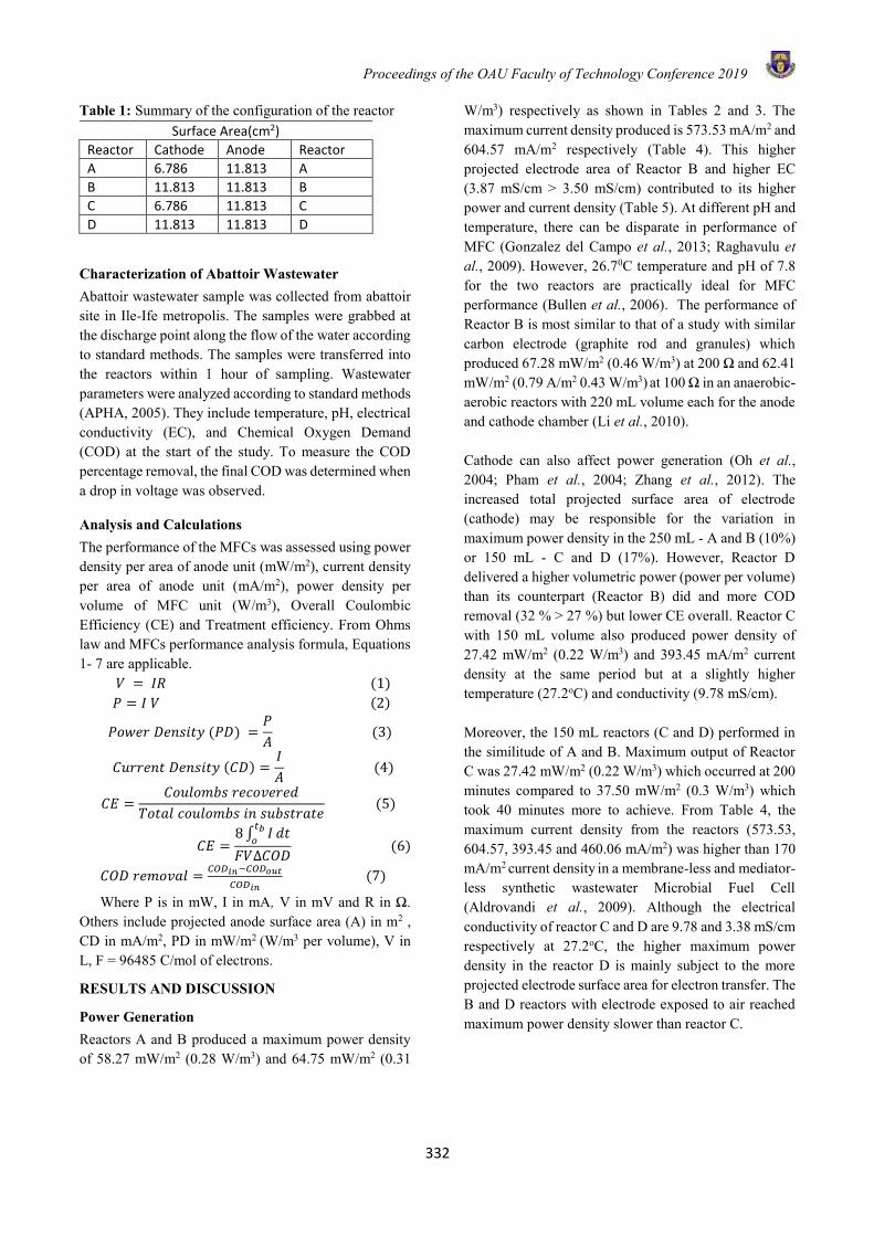
Proceedings of the OAU Faculty of Technology Conference 2019
332
Table 1: Summary of the configuration of the reactor Surface Area(cm2)
Reactor Cathode Anode Reactor
A 6.786 11.813 A
B 11.813 11.813 B
C 6.786 11.813 C
D 11.813 11.813 D
Characterization of Abattoir Wastewater Abattoir wastewater sample was collected from abattoir site in Ile-Ife metropolis. The samples were grabbed at the discharge point along the flow of the water according to standard methods. The samples were transferred into the reactors within 1 hour of sampling. Wastewater parameters were analyzed according to standard methods (APHA, 2005). They include temperature, pH, electrical conductivity (EC), and Chemical Oxygen Demand (COD) at the start of the study. To measure the COD percentage removal, the final COD was determined when a drop in voltage was observed.
Analysis and Calculations The performance of the MFCs was assessed using power density per area of anode unit (mW/m2), current density per area of anode unit (mA/m2), power density per volume of MFC unit (W/m3), Overall Coulombic Efficiency (CE) and Treatment efficiency. From Ohms law and MFCs performance analysis formula, Equations 1- 7 are applicable.
𝑉 = 𝐼𝑅 (1) 𝑃 = 𝐼 𝑉 (2)
𝑃𝑜𝑤𝑒𝑟 𝐷𝑒𝑛𝑠𝑖𝑡𝑦 (𝑃𝐷) =𝑃
𝐴 (3)
𝐶𝑢𝑟𝑟𝑒𝑛𝑡 𝐷𝑒𝑛𝑠𝑖𝑡𝑦 (𝐶𝐷) =𝐼
𝐴 (4)
𝐶𝐸 =𝐶𝑜𝑢𝑙𝑜𝑚𝑏𝑠 𝑟𝑒𝑐𝑜𝑣𝑒𝑟𝑒𝑑
𝑇𝑜𝑡𝑎𝑙 𝑐𝑜𝑢𝑙𝑜𝑚𝑏𝑠 𝑖𝑛 𝑠𝑢𝑏𝑠𝑡𝑟𝑎𝑡𝑒 (5)
𝐶𝐸 =8∫ 𝐼
𝑡𝑏𝑜
𝑑𝑡
𝐹𝑉∆𝐶𝑂𝐷 (6)
𝐶𝑂𝐷 𝑟𝑒𝑚𝑜𝑣𝑎𝑙 =𝐶𝑂𝐷𝑖𝑛−𝐶𝑂𝐷𝑜𝑢𝑡
𝐶𝑂𝐷𝑖𝑛 (7)
Where P is in mW, I in mA, V in mV and R in Ω. Others include projected anode surface area (A) in m2 , CD in mA/m2, PD in mW/m2 (W/m3 per volume), V in L, F = 96485 C/mol of electrons.
RESULTS AND DISCUSSION
Power Generation Reactors A and B produced a maximum power density of 58.27 mW/m2 (0.28 W/m3) and 64.75 mW/m2 (0.31
W/m3) respectively as shown in Tables 2 and 3. The maximum current density produced is 573.53 mA/m2 and 604.57 mA/m2 respectively (Table 4). This higher projected electrode area of Reactor B and higher EC (3.87 mS/cm > 3.50 mS/cm) contributed to its higher power and current density (Table 5). At different pH and temperature, there can be disparate in performance of MFC (Gonzalez del Campo et al., 2013; Raghavulu et al., 2009). However, 26.70C temperature and pH of 7.8 for the two reactors are practically ideal for MFC performance (Bullen et al., 2006). The performance of Reactor B is most similar to that of a study with similar carbon electrode (graphite rod and granules) which produced 67.28 mW/m2 (0.46 W/m3) at 200 Ω and 62.41 mW/m2 (0.79 A/m2 0.43 W/m3) at 100 Ω in an anaerobic-aerobic reactors with 220 mL volume each for the anode and cathode chamber (Li et al., 2010). Cathode can also affect power generation (Oh et al., 2004; Pham et al., 2004; Zhang et al., 2012). The increased total projected surface area of electrode (cathode) may be responsible for the variation in maximum power density in the 250 mL - A and B (10%) or 150 mL - C and D (17%). However, Reactor D delivered a higher volumetric power (power per volume) than its counterpart (Reactor B) did and more COD removal (32 % > 27 %) but lower CE overall. Reactor C with 150 mL volume also produced power density of 27.42 mW/m2 (0.22 W/m3) and 393.45 mA/m2 current density at the same period but at a slightly higher temperature (27.2oC) and conductivity (9.78 mS/cm). Moreover, the 150 mL reactors (C and D) performed in the similitude of A and B. Maximum output of Reactor C was 27.42 mW/m2 (0.22 W/m3) which occurred at 200 minutes compared to 37.50 mW/m2 (0.3 W/m3) which took 40 minutes more to achieve. From Table 4, the maximum current density from the reactors (573.53, 604.57, 393.45 and 460.06 mA/m2) was higher than 170 mA/m2 current density in a membrane-less and mediator-less synthetic wastewater Microbial Fuel Cell (Aldrovandi et al., 2009). Although the electrical conductivity of reactor C and D are 9.78 and 3.38 mS/cm respectively at 27.2oC, the higher maximum power density in the reactor D is mainly subject to the more projected electrode surface area for electron transfer. The B and D reactors with electrode exposed to air reached maximum power density slower than reactor C.
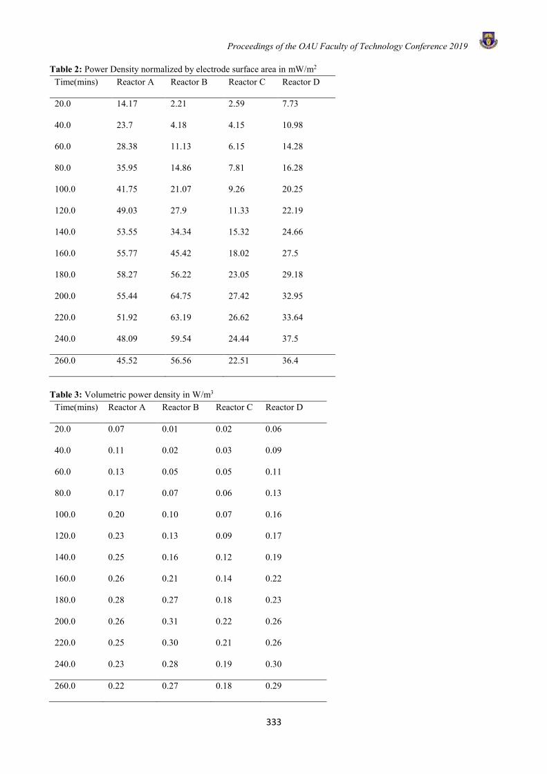
Proceedings of the OAU Faculty of Technology Conference 2019
333
Table 2: Power Density normalized by electrode surface area in mW/m2 Time(mins) Reactor A Reactor B Reactor C Reactor D
20.0 14.17 2.21 2.59 7.73
40.0 23.7 4.18 4.15 10.98
60.0 28.38 11.13 6.15 14.28
80.0 35.95 14.86 7.81 16.28
100.0 41.75 21.07 9.26 20.25
120.0 49.03 27.9 11.33 22.19
140.0 53.55 34.34 15.32 24.66
160.0 55.77 45.42 18.02 27.5
180.0 58.27 56.22 23.05 29.18
200.0 55.44 64.75 27.42 32.95
220.0 51.92 63.19 26.62 33.64
240.0 48.09 59.54 24.44 37.5
260.0 45.52 56.56 22.51 36.4
Table 3: Volumetric power density in W/m3
Time(mins) Reactor A Reactor B Reactor C Reactor D
20.0 0.07 0.01 0.02 0.06
40.0 0.11 0.02 0.03 0.09
60.0 0.13 0.05 0.05 0.11
80.0 0.17 0.07 0.06 0.13
100.0 0.20 0.10 0.07 0.16
120.0 0.23 0.13 0.09 0.17
140.0 0.25 0.16 0.12 0.19
160.0 0.26 0.21 0.14 0.22
180.0 0.28 0.27 0.18 0.23
200.0 0.26 0.31 0.22 0.26
220.0 0.25 0.30 0.21 0.26
240.0 0.23 0.28 0.19 0.30
260.0 0.22 0.27 0.18 0.29
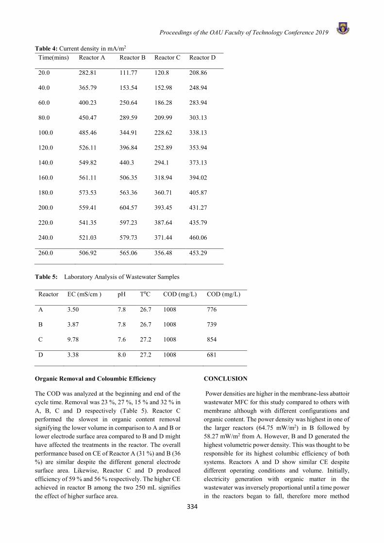
Proceedings of the OAU Faculty of Technology Conference 2019
334
Table 4: Current density in mA/m2 Time(mins) Reactor A Reactor B Reactor C Reactor D
20.0 282.81 111.77 120.8 208.86
40.0 365.79 153.54 152.98 248.94
60.0 400.23 250.64 186.28 283.94
80.0 450.47 289.59 209.99 303.13
100.0 485.46 344.91 228.62 338.13
120.0 526.11 396.84 252.89 353.94
140.0 549.82 440.3 294.1 373.13
160.0 561.11 506.35 318.94 394.02
180.0 573.53 563.36 360.71 405.87
200.0 559.41 604.57 393.45 431.27
220.0 541.35 597.23 387.64 435.79
240.0 521.03 579.73 371.44 460.06
260.0 506.92 565.06 356.48 453.29
Table 5: Laboratory Analysis of Wastewater Samples
Reactor EC (mS/cm ) pH T0C COD (mg/L) COD (mg/L)
A 3.50 7.8 26.7 1008 776
B 3.87 7.8 26.7 1008 739
C 9.78 7.6 27.2 1008 854
D 3.38 8.0 27.2 1008 681
Organic Removal and Coloumbic Efficiency
The COD was analyzed at the beginning and end of the cycle time. Removal was 23 %, 27 %, 15 % and 32 % in A, B, C and D respectively (Table 5). Reactor C performed the slowest in organic content removal signifying the lower volume in comparison to A and B or lower electrode surface area compared to B and D might have affected the treatments in the reactor. The overall performance based on CE of Reactor A (31 %) and B (36 %) are similar despite the different general electrode surface area. Likewise, Reactor C and D produced efficiency of 59 % and 56 % respectively. The higher CE achieved in reactor B among the two 250 mL signifies the effect of higher surface area.
CONCLUSION
Power densities are higher in the membrane-less abattoir wastewater MFC for this study compared to others with membrane although with different configurations and organic content. The power density was highest in one of the larger reactors (64.75 mW/m2) in B followed by 58.27 mW/m2 from A. However, B and D generated the highest volumetric power density. This was thought to be responsible for its highest columbic efficiency of both systems. Reactors A and D show similar CE despite different operating conditions and volume. Initially, electricity generation with organic matter in the wastewater was inversely proportional until a time power in the reactors began to fall, therefore more method
Proceedings of the OAU Faculty of Technology Conference 2019
335
should be devised to keep electricity production stable while simultaneously reducing the organic matter.
REFERENCES Adegbola, A. A., and Adewoye, A. O., On
Investigating Pollution of Groundwater from Atenda Abattoir Wastes, Ogbomoso, Nigeria. International Journal of Engineering and Technology, 2:122-129, 2012.
Aelterman, P., Rabaey, K., Pham, H. T., Boon, N., and Verstraete, W., Continuous electricity generation at high voltages and currents using stacked microbial fuel cells. Environmental Science and Technology, 40: 3388–3394, 2006.
Aldrovandi, A., Marsili, E., Stante, L., Paganin, P., Tabacchioni, S., and Giordano, A., Sustainable power production in a membrane-less and mediator-less synthetic wastewater microbial fuel cell. Bioresource Technology, 100: 3252–3260, 2009.
Amuda, O. S., and Alade, A., Coagulation/flocculation process in the treatment of abattoir wastewater. Desalination, 196: 22–31, 2006.
APHA. (2005), Standard Methods for the Examination of Water and Wastewater.
Bazrafshan, E., Kord Mostafapour, F., Farzadkia, M., Ownagh, K. A., and Mahvi, A. H., Slaughterhouse wastewater treatment by combined chemical coagulation and electrocoagulation process., PLos One, 7: 40108, 2012.
Bullen, R. A., Arnot, T. C., Lakeman, J. B., and Walsh, F. C., Biofuel cells and their development. Biosensors and Bioelectronics, 21: 2015–2045, 2006.
Capodaglio, A. G., Molognoni, D., Dallago, E., Liberale, A., Cella, R., Longoni, P., and Pantaleoni, L., Microbial fuel cells for direct electrical energy recovery from urban wastewaters. The Scientific World Journal, 2013: 1-8, 2013
Catal, T., Li, K., Bermek, H., and Liu, H., Electricity production from twelve monosaccharides using microbial fuel cells. Journal of Power Sources, 175: 196–200, 2008.
CES., China Environmental State Bulletin of 2012. Http,//Jcs.Mep.Gov.Cn/Hjzl/Zkgb/2012Zkgb/201306/T20130606_253418.Htm., 14, 2012
Coker, A. O., Olugasa, B. O., and Adeyemi, A. O., Abattoir wastewater quality in south western Nigeria.27th WEDC Conference on People and Systems for water, sanitation and health, 2001.
Dentel, S. K., Strogen, B., Sharma, A., and Chiu, P., Direct generation of electricity from sludges and other liquid wastes. Singapore, pp 1-34, 2004.
Ekanem, K. V., Chukwuma, G. O., and Ubah, J. I. (2016), Determination of the Physico-Chemical Characteristics of Effluent Discharged From Karu Abattoir. International Journal of Science and Technology, 5: 43–50, 2016.
Elakkiya, E., and Matheswaran, M., Comparison of anodic metabolisms in bioelectricity production during treatment of dairy wastewater in Microbial Fuel Cell. Bioresource Technology, 136: 407–412, 2013.
Feng, Y., Wang, X., Logan, B. E., and Lee, H., Brewery wastewater treatment using air-cathode microbial fuel cells. Application of Microbiology Biotechnology, 78:17-18, 2008.
Haberman, W., and Pommer, E., Biological fuel cells with sulphide storage capacity. Application of Microbiology Biotechnology, 35: 128–133, 1991.
Haoran, Y., Lifang, D., Tao, L., and Yong, C., Hydrothermal synthesis of nanostructured manganese oxide as cathodic catalyst in a microbial fuel cell fed with leachate. The Scientific World Journal, 2014: 1-11, 2014.
Hassan, I. A., Charles, C., and Ademola, T. G., Effect of Abattoir Effluent on surrounding underground water quality, A Case Study of governor road abattoir at Ikotun, Lagos state. International Journal of Advances in Pharmacy, Biology and Chemistry, 3: 23-25, 2014.
He, Z., and Angenent, L. T., Application of bacterial biocathodes in microbial fuel cells. Electroanalysis, 18: 2009–2015, 2006.
ter Heijne, A., Liu, F., Van Der Weijden, R., Wenjma, J., Buisman, C. J. N., and Hamelers, H. V. M., Copper recovery combined with electricity production in a microbial fuel cell.
Proceedings of the OAU Faculty of Technology Conference 2019
336
Environmental Science and Technology, 44: 4376–4381, 2010.
Hou, D., Lu, L., and Ren, Z. J., Microbial fuel cells and osmotic membrane bioreactors have mutual benefits for wastewater treatment and energy production. Water research, 98: 183–189, 2016.
Ismail, Z. Z., and Jaeel, A. J., Sustainable power generation in continuous flow microbial fuel cell treating actual wastewater, Influence of biocatalyst type on electricity production. The Scientific World Journal, 2013: 1-7, 2013.
Janicek, A., Fan, Y., and Liu, H., Design of microbial fuel cells for practical application, a review and analysis of scale-up studies. Biofuels, 5: 79–92, 2014.
Kim, J. R., Cheng, S., Oh, S.-E., and Logan, B. E., Power Generation Using Different Cation, Anion, and Ultrafiltration Membranes in Microbial Fuel Cells. Environmental Science and Technology, 41: 1004–1009, 2007.
Kwadzah, T. K., and Iorhemen, O. T., Assessment of the Impact of Abattoir Effluent on the Water Quality of River Kaduna, Nigeria. World Journal of Environmental Engineering, 3: 87–94, 2015.
Li, Z., Zhang, X., Lin, J., Han, S., and Lei, L., Azo dye treatment with simultaneous electricity production in an anaerobic-aerobic sequential reactor and microbial fuel cell coupled system. Bioresource Technology, 101: 4440–4445, 2010.
Liang, P., Duan, R., Jiang, Y., Zhang, X., Qiu, Y., and Huang, X., One-year operation of 1000-L modularized microbial fuel cell for municipal wastewater treatment. Water research, 141: 1–8, 2018.
Liu, H., Ramnarayanan, R., and Logan, B. E., Production of Electricity during Wastewater Treatment Using a Single Chamber Microbial Fuel Cell. Environmental Science and Technology, 38: 2281–2285, 2004.
Logan, B. E., Microbial Fuel Cells. pp. 236, 2008.
Logan, B. E., Scaling up microbial fuel cells and other bioelectrochemical systems. Application of Microbiology Biotechnology, 85: 1665–1671, 2010.
Logan, B. E., Hamelers, B., Rozendal, R., Schröder, U., Keller, J., Freguia, S., Aelterman, P., Verstraete, W., and Rabaey, K., Microbial fuel cells, Methodology and technology. Environmental Science and Technology, 1: 5181–5192, 2006.
Logan, B. E., and Liu, H., Electricity Generation Using an Air-Cathode Single Chamber Microbial Fuel Cell in the Presence and Absence of a Proton Exchange Membrane. Environmental Science and Technology, 38: 4040–4046, 2004.
Lu, N., Zhou, S.-G., Zhuang, L., Zhnag, J.-T., and Ni, J.-R., Electricity generation from starch processing wastewater using microbial fuel cell technology. Biochemical Engineering Journal, 43: 246–251, 2009.
Luo, H., Liu, G., Zhang, R., and Jin, S., Phenol degradation in microbial fuel cells. Chemical Engineering Journal, 147: 259–264, 2009.
McCarty, P. L., Bae, J., and Kim, J., Domestic wastewater treatment as a net energy producer-can this be achieved? Environmental Science and Technology, 45: 7100–7106, 2011.
Min, B., Cheng, S., and Logan, B. E., Electricity generation using membrane and salt bridge microbial fuel cells. Water Research, 39: 1675–1686, 2005a.
Min, B., Kim, J. R., Oh, S.-E., Regan, J. M., and Logan, B. E., Electricity generation from swine wastewater using microbial fuel cells. Water Research, 39: 4961–4968, 2005b.
Mohan, S., Mohanakrishna, G., Reddy, B. P., Saravanan, R., and Sarma, P. N., Bioelectricity generation from chemical wastewater treatment in mediatorless (anode) microbial fuel cell (MFC) using selectively enriched hydrogen producing mixed culture under acidophilic microenvironment. Biochemical Engineering Journal, 39: 121–130, 2008.
Neboh, H. A., Ilusanya, O. A., Ezekoye, C. C., and Orji, F. A., Assessment of Ijebu-Igbo Abattoir effluent and its impact on the ecology of the receiving soil and river. IOSR Journal of Environmental Science, Toxicology and Food Technology, 7: 61–67, 2013.
Nwanta, J. A., Onunkwo, J., and Ezenduka, E., Analysis of Nsukka Metropolitan abattoir solid waste and
Proceedings of the OAU Faculty of Technology Conference 2019
337
its bacterial contents in south eastern Nigeria, public health implications, 2016.
Oh, S.-E., and Logan, B. E., Voltage reversal during microbial fuel cell stack operation. Journal of Power Sources, 167: 11–17, 2007.
Oh, S.-E., Min, B., and Logan, B. E., Cathode performance as a factor in electricity generation in microbial fuel cells. Environmental Science and Technology, 38: 4900–4904, 2004.
Oke, I. A., Oladepo, K. T., Fehintola, E. O., Adekaunbi, E. A., Obijole, A. O., Basil, N. O., and Mohammed, H., An overview of electrochemical treatment processes in environmental engineering, modern studies on electrochemical treatment processes (2005- 2010).Water Treatment Processes, 2012.
Omole, D. O., and Longe, E. O., An Assessment of the Impact of Abattoir Effluents on River Illo, Ota, Nigeria. Journal of Environmental Science and Technology, 1: 56–64, 2008.
Patil, S. A., Surakasi, V. P., Koul, S., Ijmulwar, S., Vivek, A., Shouche, Y. S., and Kapadnis, B. P., Electricity generation using chocolate industry wastewater and its treatment in activated sludge based microbial fuel cell and analysis of developed microbial community in the anode chamber. Bioresource Technology, 100: 5132–5139, 2009.
Pham, T. H., Jang, J. K., Chang, I. S., and Kim, B. H., Improvement of cathode reaction of a mediator-less microbial fuel cell. Journal of Microbial Biotechnology, 14: 324–329, 2004.
Rabaey, K., Lissens, G., Siciliano, S. D., and Verstraete, W., A microbial fuel cell capable of converting glucose to electricity at high rate and efficiency. Biotechnology Letters, 25: 1531–1535, 2003.
Rabaey, K., and Verstraete, W., Microbial fuel cells, Novel biotechnology for energy generation. Trends in Biotechnology, 23: 291–298, 2005.
Rathore, A., Eco-Friendly Wastewater Treatment Solution Using Self-Powered Microbial Fuel Cell. International Journal of Modern Trends in Engineering and Research, 2, 2014.
Rodrigo, M. A., Cañizares, P., García, H., Linares, J. J., and Lobato, J., Study of the acclimation stage and
of the effect of the biodegradability on the performance of a microbial fuel cell. Bioresource Technology, 100: 4704–4710, 2009.
Rossi, R., Yang, W., Zikmund, E., Pant, D., and Logan, B. E., In situ biofilm removal from air cathodes in microbial fuel cells treating domestic wastewater. Bioresource technology, 265: 200–206, 2018.
Rosso, D., Strenstorm, M. K., and Larson, L. E., Aeration of large-scale municipal wastewater treatment plants, State of the art. Water Science and Technology, 57: 973–978, 2008.
Rozendal, R. A., Hamelers, H. V. M., Rabaey, K., Keller, J., and Buisman, C. J. N., Towards practical implementation of bioelectrochemical wastewater treatment. Trends in Biotechnology, 26: 450–459, 2008.
Sell, D., Kramer, P., and Kreysa, G., Use of an oxygen gas diffusion cathode and a three dimensional packed-bed anode in a bioelectrochemical fuel cell. Application of Microbiology Biotechnology, 31: 211–213, 1989.
Wang, H., and Ren, Z. J., A comprehensive review of microbial electrochemical systems as a platform technology. Biotechnology Advances, 31: 1796–1807, 2013.
Wang, X., Feng, Y. J., and Lee, H., Electricity production from beer brewery wastewater using single chamber microbial fuel cell. Water Science and Technology, 57: 1117–1121, 2008.
Wen, Q., Wu, Y., Cao, D., Zhao, L., and Sun, Q., Electricity generation and modeling of microbial fuel cell from continuous beer brewery wastewater. Bioresource Technology, 100: 4171–4175, 2009.
Yang, N., Zhan, G., Li, D., Wang, X., He, X., and Liu, H., Complete nitrogen removal and electricity production in Thauera-dominated air-cathode single chambered microbial fuel cell. Chemical Engineering Journal, 356: 506–515, 2019.
Yuan, H. R., Deng, L. F., Chen, Y., and Zhou, S. G., Electricity generation from municipal solid waste leachate using microbial fuel cell technology. Journal of Basic Science and Engineering, 20: 800–810, 2012.
Zhang, E., Xu, W., Diao, G., and Shuang, C., Electricity generation from acetate and glucose by

Proceedings of the OAU Faculty of Technology Conference 2019
338
sedimentary bacterium attached to electrode in microbial-anode fuel cells. Journal of Power Sources, 161: 820–825, 2006.
Zhang, G., Wang, K., Zhao, Q., Jiao, Y., and Lee, D., Effect of cathode types on long-term performance and anode bacterial communities in microbial fuel cells. Bioresource Technology, 118: 249–256, 2012.
Zuo, Y., Cheng, S., Call, D., and Logan, B. E., Tubular membrane cathodes for scalable power generation in microbial fuel cells. Environmental Science and Technology, 41: 3347–3353, 2007.
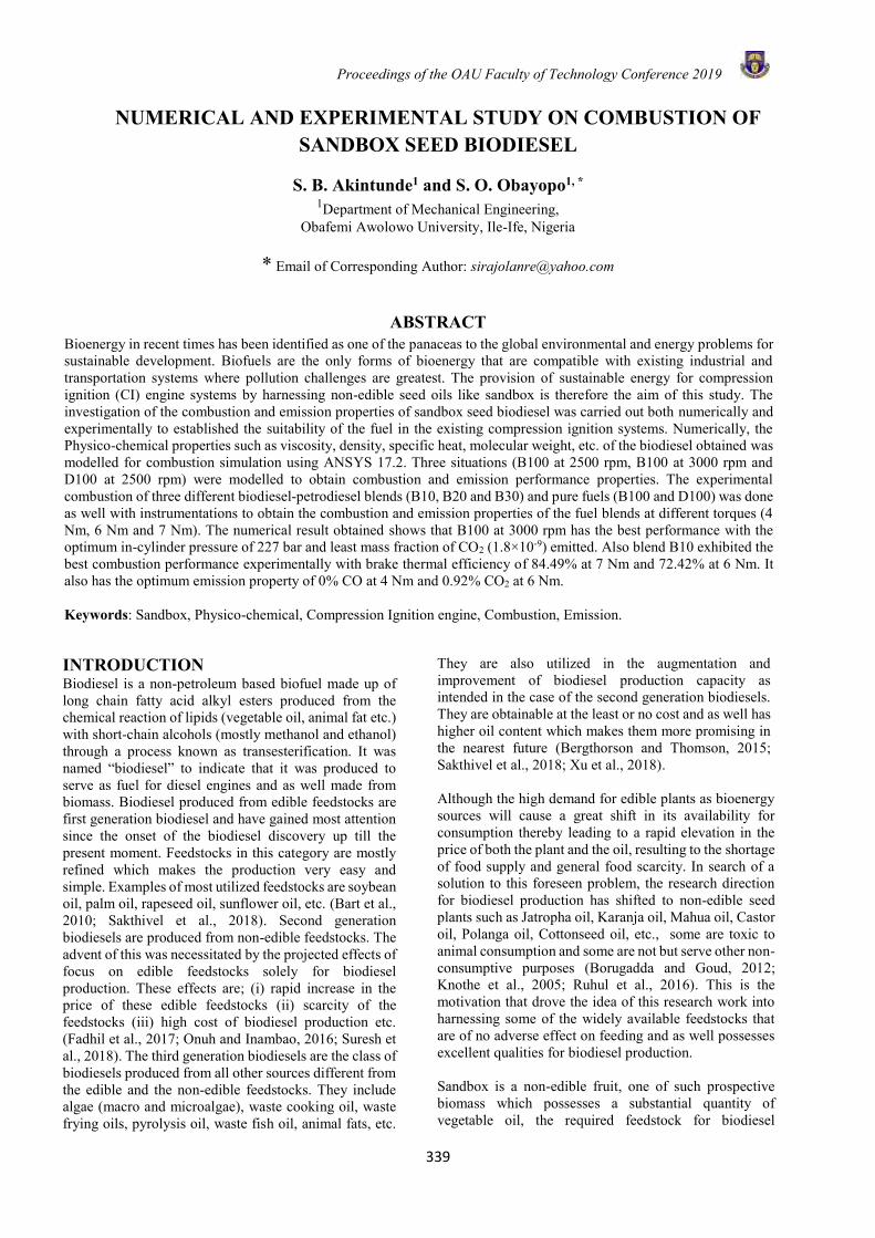
Proceedings of the OAU Faculty of Technology Conference 2019
339
NUMERICAL AND EXPERIMENTAL STUDY ON COMBUSTION OF SANDBOX SEED BIODIESEL
S. B. Akintunde1 and S. O. Obayopo1, * 1Department of Mechanical Engineering,
Obafemi Awolowo University, Ile-Ife, Nigeria
* Email of Corresponding Author: [email protected]
ABSTRACT Bioenergy in recent times has been identified as one of the panaceas to the global environmental and energy problems for sustainable development. Biofuels are the only forms of bioenergy that are compatible with existing industrial and transportation systems where pollution challenges are greatest. The provision of sustainable energy for compression ignition (CI) engine systems by harnessing non-edible seed oils like sandbox is therefore the aim of this study. The investigation of the combustion and emission properties of sandbox seed biodiesel was carried out both numerically and experimentally to established the suitability of the fuel in the existing compression ignition systems. Numerically, the Physico-chemical properties such as viscosity, density, specific heat, molecular weight, etc. of the biodiesel obtained was modelled for combustion simulation using ANSYS 17.2. Three situations (B100 at 2500 rpm, B100 at 3000 rpm and D100 at 2500 rpm) were modelled to obtain combustion and emission performance properties. The experimental combustion of three different biodiesel-petrodiesel blends (B10, B20 and B30) and pure fuels (B100 and D100) was done as well with instrumentations to obtain the combustion and emission properties of the fuel blends at different torques (4 Nm, 6 Nm and 7 Nm). The numerical result obtained shows that B100 at 3000 rpm has the best performance with the optimum in-cylinder pressure of 227 bar and least mass fraction of CO2 (1.8×10⁻⁹) emitted. Also blend B10 exhibited the best combustion performance experimentally with brake thermal efficiency of 84.49% at 7 Nm and 72.42% at 6 Nm. It also has the optimum emission property of 0% CO at 4 Nm and 0.92% CO2 at 6 Nm. Keywords: Sandbox, Physico-chemical, Compression Ignition engine, Combustion, Emission.
INTRODUCTION Biodiesel is a non-petroleum based biofuel made up of long chain fatty acid alkyl esters produced from the chemical reaction of lipids (vegetable oil, animal fat etc.) with short-chain alcohols (mostly methanol and ethanol) through a process known as transesterification. It was named “biodiesel” to indicate that it was produced to serve as fuel for diesel engines and as well made from biomass. Biodiesel produced from edible feedstocks are first generation biodiesel and have gained most attention since the onset of the biodiesel discovery up till the present moment. Feedstocks in this category are mostly refined which makes the production very easy and simple. Examples of most utilized feedstocks are soybean oil, palm oil, rapeseed oil, sunflower oil, etc. (Bart et al., 2010; Sakthivel et al., 2018). Second generation biodiesels are produced from non-edible feedstocks. The advent of this was necessitated by the projected effects of focus on edible feedstocks solely for biodiesel production. These effects are; (i) rapid increase in the price of these edible feedstocks (ii) scarcity of the feedstocks (iii) high cost of biodiesel production etc. (Fadhil et al., 2017; Onuh and Inambao, 2016; Suresh et al., 2018). The third generation biodiesels are the class of biodiesels produced from all other sources different from the edible and the non-edible feedstocks. They include algae (macro and microalgae), waste cooking oil, waste frying oils, pyrolysis oil, waste fish oil, animal fats, etc.
They are also utilized in the augmentation and improvement of biodiesel production capacity as intended in the case of the second generation biodiesels. They are obtainable at the least or no cost and as well has higher oil content which makes them more promising in the nearest future (Bergthorson and Thomson, 2015; Sakthivel et al., 2018; Xu et al., 2018). Although the high demand for edible plants as bioenergy sources will cause a great shift in its availability for consumption thereby leading to a rapid elevation in the price of both the plant and the oil, resulting to the shortage of food supply and general food scarcity. In search of a solution to this foreseen problem, the research direction for biodiesel production has shifted to non-edible seed plants such as Jatropha oil, Karanja oil, Mahua oil, Castor oil, Polanga oil, Cottonseed oil, etc., some are toxic to animal consumption and some are not but serve other non-consumptive purposes (Borugadda and Goud, 2012; Knothe et al., 2005; Ruhul et al., 2016). This is the motivation that drove the idea of this research work into harnessing some of the widely available feedstocks that are of no adverse effect on feeding and as well possesses excellent qualities for biodiesel production. Sandbox is a non-edible fruit, one of such prospective biomass which possesses a substantial quantity of vegetable oil, the required feedstock for biodiesel
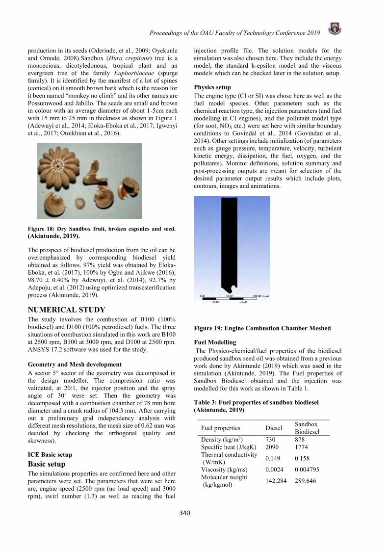
Proceedings of the OAU Faculty of Technology Conference 2019
340
production in its seeds (Oderinde, et al., 2009; Oyekunle and Omode, 2008).Sandbox (Hura crepitans) tree is a monoecious, dicotyledonous, tropical plant and an evergreen tree of the family Euphorbiaceae (spurge family). It is identified by the manifest of a lot of spines (conical) on it smooth brown bark which is the reason for it been named “monkey no climb” and its other names are Possumwood and Jabillo. The seeds are small and brown in colour with an average diameter of about 1-5cm each with 15 mm to 25 mm in thickness as shown in Figure 1 (Adewuyi et al., 2014; Eloka-Eboka et al., 2017; Igwenyi et al., 2017; Otoikhian et al., 2016).
Figure 18: Dry Sandbox fruit, broken capsules and seed. (Akintunde, 2019).
The prospect of biodiesel production from the oil can be overemphasized by corresponding biodiesel yield obtained as follows. 97% yield was obtained by Eloka-Eboka, et al. (2017), 100% by Ogbu and Ajikwe (2016), 98.70 ± 0.40% by Adewuyi, et al. (2014), 92.7% by Adepoju, et al. (2012) using optimized transesterification process (Akintunde, 2019).
NUMERICAL STUDY The study involves the combustion of B100 (100% biodiesel) and D100 (100% petrodiesel) fuels. The three situations of combustion simulated in this work are B100 at 2500 rpm, B100 at 3000 rpm, and D100 at 2500 rpm. ANSYS 17.2 software was used for the study. Geometry and Mesh development A sector 5° sector of the geometry was decomposed in the design modeller. The compression ratio was validated, at 20:1, the injector position and the spray angle of 30˚ were set. Then the geometry was decomposed with a combustion chamber of 78 mm bore diameter and a crank radius of 104.3 mm. After carrying out a preliminary grid independency analysis with different mesh resolutions, the mesh size of 0.62 mm was decided by checking the orthogonal quality and skewness).
ICE Basic setup Basic setup The simulations properties are confirmed here and other parameters were set. The parameters that were set here are, engine speed (2500 rpm (no load speed) and 3000 rpm), swirl number (1.3) as well as reading the fuel
injection profile file. The solution models for the simulation was also chosen here. They include the energy model, the standard k-epsilon model and the viscous models which can be checked later in the solution setup.
Physics setup The engine type (CI or SI) was chose here as well as the fuel model species. Other parameters such as the chemical reaction type, the injection parameters (and fuel modelling in CI engines), and the pollutant model type (for soot, NOX etc.) were set here with similar boundary conditions to Govindal et al., 2014 (Govindan et al., 2014). Other settings include initialization (of parameters such as gauge pressure, temperature, velocity, turbulent kinetic energy, dissipation, the fuel, oxygen, and the pollutants). Monitor definitions, solution summary and post-processing outputs are meant for selection of the desired parameter output results which include plots, contours, images and animations.
Figure 19: Engine Combustion Chamber Meshed
Fuel Modelling The Physico-chemical/fuel properties of the biodiesel produced sandbox seed oil was obtained from a previous work done by Akintunde (2019) which was used in the simulation (Akintunde, 2019). The Fuel properties of Sandbox Biodiesel obtained and the injection was modelled for this work as shown in Table 1.
Table 3: Fuel properties of sandbox biodiesel (Akintunde, 2019)
Fuel properties Diesel Sandbox Biodiesel
Density (kg/m3) 730 878 Specific heat (J/kgK) 2090 1774 Thermal conductivity (W/mK) 0.149 0.158
Viscosity (kg/ms) 0.0024 0.004795 Molecular weight (kg/kgmol)
142.284 289.646
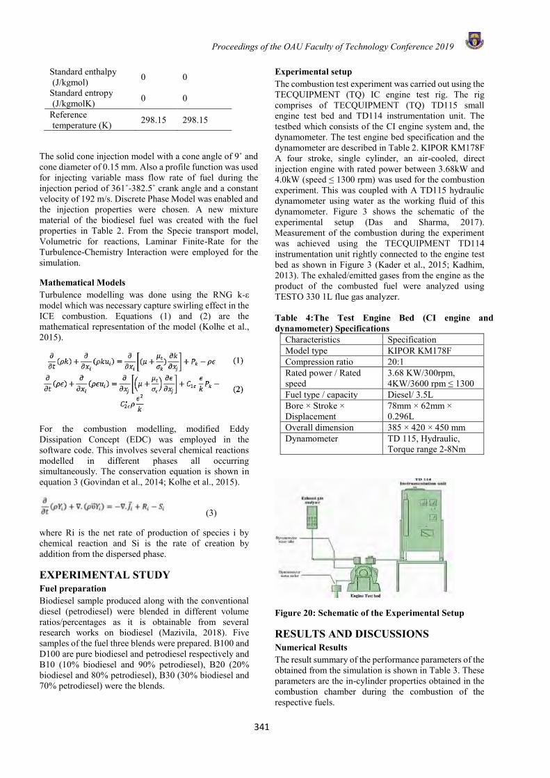
Proceedings of the OAU Faculty of Technology Conference 2019
341
Standard enthalpy (J/kgmol)
0 0
Standard entropy (J/kgmolK) 0 0
Reference temperature (K) 298.15 298.15
The solid cone injection model with a cone angle of 9˚ and cone diameter of 0.15 mm. Also a profile function was used for injecting variable mass flow rate of fuel during the injection period of 361˚-382.5˚ crank angle and a constant velocity of 192 m/s. Discrete Phase Model was enabled and the injection properties were chosen. A new mixture material of the biodiesel fuel was created with the fuel properties in Table 2. From the Specie transport model, Volumetric for reactions, Laminar Finite-Rate for the Turbulence-Chemistry Interaction were employed for the simulation.
Mathematical Models Turbulence modelling was done using the RNG k-ε model which was necessary capture swirling effect in the ICE combustion. Equations (1) and (2) are the mathematical representation of the model (Kolhe et al., 2015).
For the combustion modelling, modified Eddy Dissipation Concept (EDC) was employed in the software code. This involves several chemical reactions modelled in different phases all occurring simultaneously. The conservation equation is shown in equation 3 (Govindan et al., 2014; Kolhe et al., 2015).
(3)
where Ri is the net rate of production of species i by chemical reaction and Si is the rate of creation by addition from the dispersed phase.
EXPERIMENTAL STUDY Fuel preparation Biodiesel sample produced along with the conventional diesel (petrodiesel) were blended in different volume ratios/percentages as it is obtainable from several research works on biodiesel (Mazivila, 2018). Five samples of the fuel three blends were prepared. B100 and D100 are pure biodiesel and petrodiesel respectively and B10 (10% biodiesel and 90% petrodiesel), B20 (20% biodiesel and 80% petrodiesel), B30 (30% biodiesel and 70% petrodiesel) were the blends.
Experimental setup The combustion test experiment was carried out using the TECQUIPMENT (TQ) IC engine test rig. The rig comprises of TECQUIPMENT (TQ) TD115 small engine test bed and TD114 instrumentation unit. The testbed which consists of the CI engine system and, the dynamometer. The test engine bed specification and the dynamometer are described in Table 2. KIPOR KM178F A four stroke, single cylinder, an air-cooled, direct injection engine with rated power between 3.68kW and 4.0kW (speed ≤ 1300 rpm) was used for the combustion experiment. This was coupled with A TD115 hydraulic dynamometer using water as the working fluid of this dynamometer. Figure 3 shows the schematic of the experimental setup (Das and Sharma, 2017). Measurement of the combustion during the experiment was achieved using the TECQUIPMENT TD114 instrumentation unit rightly connected to the engine test bed as shown in Figure 3 (Kader et al., 2015; Kadhim, 2013). The exhaled/emitted gases from the engine as the product of the combusted fuel were analyzed using TESTO 330 1L flue gas analyzer. Table 4:The Test Engine Bed (CI engine and dynamometer) Specifications
Characteristics Specification Model type KIPOR KM178F Compression ratio 20:1 Rated power / Rated speed
3.68 KW/300rpm, 4KW/3600 rpm ≤ 1300
Fuel type / capacity Diesel/ 3.5L Bore × Stroke × Displacement
78mm × 62mm × 0.296L
Overall dimension 385 × 420 × 450 mm Dynamometer TD 115, Hydraulic,
Torque range 2-8Nm
Figure 20: Schematic of the Experimental Setup
RESULTS AND DISCUSSIONS Numerical Results The result summary of the performance parameters of the obtained from the simulation is shown in Table 3. These parameters are the in-cylinder properties obtained in the combustion chamber during the combustion of the respective fuels.
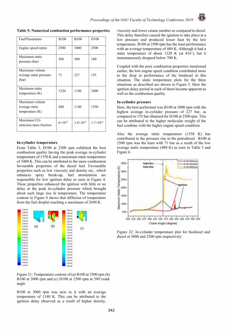
Proceedings of the OAU Faculty of Technology Conference 2019
342
Table 5: Numerical combustion performance properties
Fuel/Parameters B100 B100 D100
Engine speed (rpm) 2500 3000 2500
Maximum static pressure (bar)
500 500 180
Maximum volume average static pressure (bar)
71 227 155
Maximum static temperature (K)
1220 1180 3400
Maximum volume average static temperature (K)
480 1140 1550
Maximum CO2 emission mass fraction
6×10⁻⁹ 1.8×10⁻⁹ 1.7×10⁻⁶
In-cylinder temperature From Table 3, D100 at 2500 rpm exhibited the best combustion quality having the peak average in-cylinder temperature of 1550 K and a maximum static temperature of 3400 K. This can be attributed to the more combustion favourable properties of the diesel fuel. Favourable properties such as low viscosity and density etc., which enhances spray break-up, fuel atomization are responsible for low ignition delay as seen in Figure 4. These properties enhanced the ignition with little or no delay at the peak in-cylinder pressure which brought about such large rise in temperature. The temperature contour in Figure 4 shows that diffusion of temperature from the fuel droplet reaching a maximum of 2690 K.
Figure 21: Temperature contour of (a) B100 at 2500 rpm (b) B100 at 3000 rpm and (c) D100 at 2500 rpm at 390˚crank angle
B100 at 3000 rpm was next to it with an average temperature of 1140 K. This can be attributed to the ignition delay observed as a result of higher density,
viscosity and lower cetane number as compared to diesel. This delay therefore caused the ignition to take place at a low pressure and produced lesser heat by the low temperature. B100 at 2500 rpm has the least performance with an average temperature of 480 K. Although it had a static temperature of about 1220 K (at 416˚), but it instantaneously dropped below 700 K.
Coupled with the poor combustion properties mentioned earlier, the low engine speed condition contributed more to the drop in performance of the biodiesel in this situation. The static temperature plots for the three situations as described are shown in Figure 5. Here the ignition delay period in each of them became apparent as well as the combustion quality.
In-cylinder pressure Here, the best performed was B100 at 3000 rpm with the highest average in-cylinder pressure of 227 bar, as compared to 155 bar obtained for D100 at 2500 rpm. This can be attributed to the higher molecular weight of the fuel combine with the higher engine speed condition.
Also the average static temperature (1550 K) has contributed to the pressure rise in the petrodiesel. B100 at 2500 rpm was the least with 71 bar as a result of the low average static temperature (480 K) as seen in Table 3 and Figure 6.
Figure 22: In-cylinder temperature plot for biodiesel and diesel at 3000 and 2500 rpm respectively
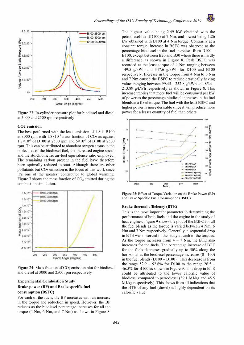
Proceedings of the OAU Faculty of Technology Conference 2019
343
Figure 23: In-cylinder pressure plot for biodiesel and diesel at 3000 and 2500 rpm respectively
CO2 emission The best performed with the least emission of 1.8 is B100 at 3000 rpm with 1.8×10⁻⁹ mass fraction of CO2 as against 1.7×10⁻⁶ of D100 at 2500 rpm and 6×10⁻⁹ of B100 at 2500 rpm. This can be attributed to abundant oxygen atoms in the molecules of the biodiesel fuel, the increased engine speed and the stoichiometric air-fuel equivalence ratio employed. The remaining carbon present in the fuel have therefore been optimally reduced to soot. Although there are other pollutants but CO2 emission is the focus of this work since it’s one of the greatest contributor to global warming. Figure 7 shows the mass fraction of CO2 emitted during the combustion simulation.
Figure 24: Mass fraction of CO2 emission plot for biodiesel and diesel at 3000 and 2500 rpm respectively
Experimental Combustion Study Brake power (BP) and Brake specific fuel consumption (BSFC) For each of the fuels, the BP increases with an increase in the torque and reduction in speed. However, the BP reduces as the biodiesel percentage increases for all the torque (4 Nm, 6 Nm, and 7 Nm) as shown in Figure 8.
The highest value being 2.49 kW obtained with the petrodiesel fuel (D100) at 7 Nm, and lowest being 1.26 kW obtained with B100 at 4 Nm torque. Contrarily at a constant torque, increase in BSFC was observed as the percentage biodiesel in the fuel increases from D100 – B100, except between B20 and B30 where there is hardly a difference as shown in Figure 8. Peak BSFC was recorded at the least torque of 4 Nm ranging between 149.5 g/kWh and 347.6 g/kWh for D100 and B100 respectively. Increase in the torque from 4 Nm to 6 Nm and 7 Nm caused the BSFC to reduce drastically having values ranging between 99.45 – 252.8 g/kWh and 85.4 – 213.89 g/kWh respectively as shown in Figure 8. This increase implies that more fuel will be consumed per kW of power as the percentage biodiesel increases in the fuel blends at a fixed torque. The fuel with the least BSFC and higher power is more desirable since it will produce more power for a lesser quantity of fuel than others.
Figure 25: Effect of Torque Variation on the Brake Power (BP) and Brake Specific Fuel Consumption (BSFC)
Brake thermal efficiency (BTE) This is the most important parameter in determining the performance of both fuels and the engine in the study of heat engines. Figure 9 shows the plot of the BSFC for all the fuel blends as the torque is varied between 4 Nm, 6 Nm and 7 Nm respectively. Generally, a sequential drop in BTE was observed in the study at each of the torques. As the torque increases from 4 – 7 Nm, the BTE also increases for the fuels. The percentage increase of BTE for the fuels decreases gradually up to 50% along the horizontal as the biodiesel percentage increases (0 - 100) in the fuel blends (D100 – B100). This decrease is from the range 52.9 – 92.6% for D100 to the range 26.5 – 46.5% for B100 as shown in Figure 9. This drop in BTE could be attributed to the lower calorific value of biodiesel compared to petrodiesel (39.1 MJ/kg and 45.5 MJ/kg respectively). This shows from all indications that the BTE of any fuel (diesel) is highly dependent on its calorific value.
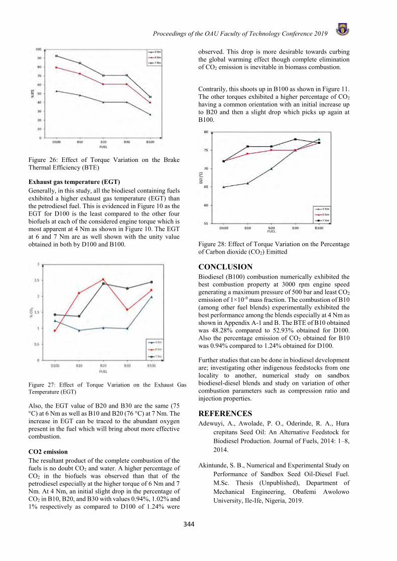
Proceedings of the OAU Faculty of Technology Conference 2019
344
Figure 26: Effect of Torque Variation on the Brake Thermal Efficiency (BTE)
Exhaust gas temperature (EGT) Generally, in this study, all the biodiesel containing fuels exhibited a higher exhaust gas temperature (EGT) than the petrodiesel fuel. This is evidenced in Figure 10 as the EGT for D100 is the least compared to the other four biofuels at each of the considered engine torque which is most apparent at 4 Nm as shown in Figure 10. The EGT at 6 and 7 Nm are as well shown with the unity value obtained in both by D100 and B100.
Figure 27: Effect of Torque Variation on the Exhaust Gas Temperature (EGT)
Also, the EGT value of B20 and B30 are the same (75 °C) at 6 Nm as well as B10 and B20 (76 °C) at 7 Nm. The increase in EGT can be traced to the abundant oxygen present in the fuel which will bring about more effective combustion. CO2 emission The resultant product of the complete combustion of the fuels is no doubt CO2 and water. A higher percentage of CO2 in the biofuels was observed than that of the petrodiesel especially at the higher torque of 6 Nm and 7 Nm. At 4 Nm, an initial slight drop in the percentage of CO2 in B10, B20, and B30 with values 0.94%, 1.02% and 1% respectively as compared to D100 of 1.24% were
observed. This drop is more desirable towards curbing the global warming effect though complete elimination of CO2 emission is inevitable in biomass combustion.
Contrarily, this shoots up in B100 as shown in Figure 11. The other torques exhibited a higher percentage of CO2 having a common orientation with an initial increase up to B20 and then a slight drop which picks up again at B100.
Figure 28: Effect of Torque Variation on the Percentage of Carbon dioxide (CO2) Emitted
CONCLUSION Biodiesel (B100) combustion numerically exhibited the best combustion property at 3000 rpm engine speed generating a maximum pressure of 500 bar and least CO2 emission of 1×10⁻⁹ mass fraction. The combustion of B10 (among other fuel blends) experimentally exhibited the best performance among the blends especially at 4 Nm as shown in Appendix A-1 and B. The BTE of B10 obtained was 48.28% compared to 52.93% obtained for D100. Also the percentage emission of CO2 obtained for B10 was 0.94% compared to 1.24% obtained for D100.
Further studies that can be done in biodiesel development are; investigating other indigenous feedstocks from one locality to another, numerical study on sandbox biodiesel-diesel blends and study on variation of other combustion parameters such as compression ratio and injection properties.
REFERENCES Adewuyi, A., Awolade, P. O., Oderinde, R. A., Hura
crepitans Seed Oil: An Alternative Feedstock for Biodiesel Production. Journal of Fuels, 2014: 1–8, 2014.
Akintunde, S. B., Numerical and Experimental Study on Performance of Sandbox Seed Oil-Diesel Fuel. M.Sc. Thesis (Unpublished), Department of Mechanical Engineering, Obafemi Awolowo University, Ile-Ife, Nigeria, 2019.
Proceedings of the OAU Faculty of Technology Conference 2019
345
Bart, J. C. J., Natale Palmeri, Stefano Cavallaro., Biodiesel science and technology. Woodhead Publishing Series in Energy, Woodhead Publishing Limited, Cambridge, 2010.
Bergthorson, J. M., Thomson, M. J., A review of the combustion and emissions properties of advanced transportation biofuels and their impact on existing and future engines. Renewable and Sustainable Energy Reviews, 42: 1393–1417, 2015.
Borugadda, V. B., Goud, V. V., Biodiesel production from renewable feedstocks: Status and opportunities. Renewable and Sustainable Energy Reviews, 16(7): 4763–4784, 2012.
Eloka-Eboka, A. C., Igbum, G. O., Inambao, F. L., Biodiesel methyl ester production and testing from selected African tropical seed oil feedstocks. Energy Procedia, 142: 755–767, 2017.
Fadhil, A. B., Al-Tikrity, E. T. B., Albadree, M. A., Biodiesel production from mixed non-edible oils, castor seed oil and waste fish oil. Fuel, pp. 721–728, 2017.
Govindan, R., O. P. Jakha, Y. B. Mathur., Computational Analysis of Thumba Biodiesel-Diesel Blends Combustion in CI Engine Using Ansys- Fluent. International Journal of Computer & Mathematical Sciences, 3(8): 29–39, 2014.
Igwenyi, I. O., Enyi, N. A., Igwenyi, I. P., Famurewa, A. C., Obasi, N. A., Amino acid composition, fatty acid profile and characterization of vegetable oil from Hura crepitans seed. International Journal of Biology, Pharmacy and Allied Sciences, 6(9): 1781–1791, 2017.
Kader, F., Noor-e-Mostofa, A., Shuvo, A. R. M., Study of IC engine performance using different fuels. Continental Journal of Engineering Technology and Innovation, l(1): 1–9, 2015.
Kadhim, N. S., Experimental Investigation of Three Various Sources of Diesel Fuel on the Engine Performance. Journal of Babylon University/Pure and Applied Sciences, 21(8): 2955–2964, 2013.
Knothe, G., Gerpen, J. V., Krahl, J., The Biodiesel Handbook. AOCS Press, Champaign, Illinois, 2005.
Kolhe, A. V., Shelke, R. E., Khandare, S. S., Combustion Modeling with CFD in Direct Injection CI Engine
Fueled with Biodiesel. Jordan Journal of Mechanical and Industrial Engineering (JJMIE), 9(1): 61–66, 2015.
Mazivila, S. J., Trends of non-destructive analytical methods for identification of biodiesel feedstock in diesel-biodiesel blend according to European Commission Directive 2012/0288/EC and detecting diesel-biodiesel blend adulteration: A brief review. Talanta. Elsevier B.V. Talanta, 180: 239–247, 2018.
Oderinde, R. A., Ajayi, I. A., Adewuyi, A., Characterization of seed and seed oil of Hura crepitans and the kinetics of degradation of the oil during heating. Electronic Journal of Environmental, Agricultural and Food Chemistry, 8(3): 201–208, 2009.
Onuh, E. I., Inambao, F., Performance and emission evaluation of pure biodiesel from non-edible feedstock and waste oil in a diesel engine. African Journal of Science, Technology, Innovation and Development, 8(5–6): 387–398, 2016.
Otoikhian, S. K., Aluyor, E. O., Audu, T. O. K., Chemical Technology: An Indian Journal Mechanical Extraction and Fuel Properties Evaluation of Hura crepitans. Chemical Technology, 11(6): 1–11, 2016.
Oyekunle, J. A. O., Omode, A. A., Chemical composition and fatty acid profile of the lipid fractions of selected Nigerian indigenous oilseeds. International Journal of Food Properties, 11(2): 273–281, 2008.
Ruhul, A. M., Masjuki, H. H., Kalam, M. A., Shahir, S. A., Reham, S. S., Shancita, I., Biodiesel production, properties and emissions test characteristics of non‐edible fuels in Diesel engine. Journal of Scientific Research and Development, 3(1): 101–106, 2016.
Sakthivel, R., Ramesh, K., Purnachandran, R., Mohamed, S. P., A review on the properties, performance and emission aspects of the third generation biodiesels. Renewable and Sustainable Energy Reviews, 82(5): 2970–2992, 2018.
Suresh, M., Jawahar, C. P., Richard, A., A review on biodiesel production, combustion, performance, and emission characteristics of non-edible oils in variable compression ratio diesel engine using

Proceedings of the OAU Faculty of Technology Conference 2019
346
biodiesel and its blends. Renewable and Sustainable Energy Reviews, 92: 38–49, 2018.
Xu, K., Lv, B., Huo, Y.-X., Li, C., Toward the lowest energy consumption and emission in biofuel production: combination of ideal reactors and robust hosts. Current Opinion in Biotechnology, 50: 19–24, 2018.
Proceedings of the OAU Faculty of Technology Conference 2019
347
DESIGN AND IMPLEMENTATION OF ENHANCED VEHICLE ANTI-THEFT SYSTEM
F. O. ASAHIAH and O. E. ODUJOBI Department of Computer Science and Engineering,
Obafemi Awolowo University, Ile-Ife, Nigeria
* Email of Corresponding Author: [email protected];
ABSTRACT Abstract Vehicle anti-theft system which is remotely controlled via GSM network is a system that utilizes the GSM network and embedded system design in order to produce a real-time, reliable and efficient vehicle security system. It uses the GSM modem to communication between the user and the proposed system through short message services (SMS). The project consists of both hardware and software parts. The hardware components include a PIC16F876A microcontroller, relay, ignition lock, a GSM modem, Liquid Crystal Display (LCD) and a buzzer. The software is a program controller interface built with MikroC programming language. The GSM modem is controlled using the AT COMMAND and the microcontroller. The system was tested for latency, accuracy and availability. The latency was 7 seconds while the accuracy was 100%. Availability, however, depends on network of pre-configure SIM card. The vehicle anti-theft system prototype achieved its goals by preventing the ignition from starting the car without authorization after communication between the system and the owner’s phone via SMS.
Keywords: GSM, LCD, Microcontroller, SMS, Vehicle Anti-Theft
INTRODUCTION Many times we hear the cases of vehicles getting stolen from parking area or sometimes we forgot to remove the keys from vehicles by mistake. The volume of vehicle theft is a serious challenge all around the world. With the increasing vehicle theft, the prime concern for vehicle safety is arising. There are existing solutions that attempts to address this problem in various ways The importance of this project cannot be over emphasized since it helps to reduce the rate of vehicle theft within our society. According to UN-CTS M4.4, 'Motor Vehicle Theft' means the unauthorized removal of a motor vehicle without the owner’s consent. 'Motor Vehicles' includes all road-based machines with an engine used for transporting people or goods. This definition covers cars, motorcycles, carts buses, lorries and agricultural vehicles. According to statistics from United Nations Office on Drugs and Crime (UNODC), the rate of motor vehicle theft in Nigeria for year 2013 was 1.2 cases per 100,000. UNODC in its online publication for a total theft volume of 2043 cases. In the United States, finding indicated that 229,339 vehicle with keys or fobs left in the vehicles in the space of two years from January 1, 2016 to December 31, 2018. This is an increase of 56% in vehicle thefts with keys or fobs in the vehicle compared to same length of time from January 1, 2013 to December 31, 2015. The Punch Newspaper of Novembers 26, 2017 reported that theft of cars uses relay technology to simulate the presence of key in United Kingdom. In the Federal Capital Territory, Abuja, Nigeria, The Nigerian Police indicated that most
stolen vehicles were removed from the parking lot. (Punch, September 29, 2017). Most of the existing solutions to vehicle theft relies on the either preventing entry or engine start up without notifying the owner of such attempt at real time. The proposed system could be used alone or to complement existing solutions by providing mechanism that requires car owner to approve engine start up apart from having the required ignition key. The remainder of the paper consist of review of literature, a description of proposed system and its implementation. We concluded with a recommendation REVIEW OF EXISTING WORK Lili & Tiejun (2009) proposed a two layer car security system. The first layer detects forceful intrusion into the vehicle and alerts the car owner via a short message service from integrated GSM module. The owner was then expected to intervene by sending command to prevent movement. The second layer of their proposed system is activated if there is no response and the car speed passed a certain threshold. Verma & Bhatia (2013) developed a vehicle route monitoring system that can trace the route taken by a vehicle on a Google Map, reporting the information to a remote location via a web interface. The developed system can also report the exact location of vehicle (Bhatia & Verma, 2013). Many other GSM alert and monitoring system are basically concerned with the
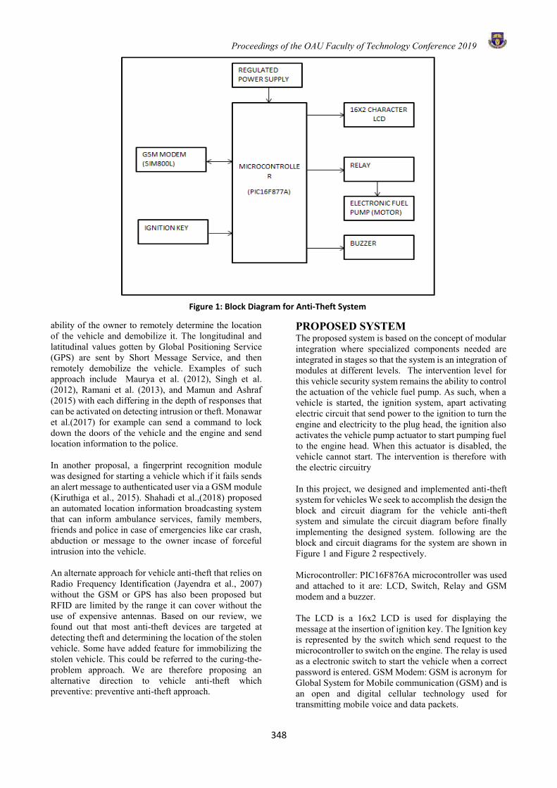
Proceedings of the OAU Faculty of Technology Conference 2019
348
ability of the owner to remotely determine the location of the vehicle and demobilize it. The longitudinal and latitudinal values gotten by Global Positioning Service (GPS) are sent by Short Message Service, and then remotely demobilize the vehicle. Examples of such approach include Maurya et al. (2012), Singh et al. (2012), Ramani et al. (2013), and Mamun and Ashraf (2015) with each differing in the depth of responses that can be activated on detecting intrusion or theft. Monawar et al.(2017) for example can send a command to lock down the doors of the vehicle and the engine and send location information to the police. In another proposal, a fingerprint recognition module was designed for starting a vehicle which if it fails sends an alert message to authenticated user via a GSM module (Kiruthiga et al., 2015). Shahadi et al.,(2018) proposed an automated location information broadcasting system that can inform ambulance services, family members, friends and police in case of emergencies like car crash, abduction or message to the owner incase of forceful intrusion into the vehicle. An alternate approach for vehicle anti-theft that relies on Radio Frequency Identification (Jayendra et al., 2007) without the GSM or GPS has also been proposed but RFID are limited by the range it can cover without the use of expensive antennas. Based on our review, we found out that most anti-theft devices are targeted at detecting theft and determining the location of the stolen vehicle. Some have added feature for immobilizing the stolen vehicle. This could be referred to the curing-the-problem approach. We are therefore proposing an alternative direction to vehicle anti-theft which preventive: preventive anti-theft approach.
PROPOSED SYSTEM The proposed system is based on the concept of modular integration where specialized components needed are integrated in stages so that the system is an integration of modules at different levels. The intervention level for this vehicle security system remains the ability to control the actuation of the vehicle fuel pump. As such, when a vehicle is started, the ignition system, apart activating electric circuit that send power to the ignition to turn the engine and electricity to the plug head, the ignition also activates the vehicle pump actuator to start pumping fuel to the engine head. When this actuator is disabled, the vehicle cannot start. The intervention is therefore with the electric circuitry In this project, we designed and implemented anti-theft system for vehicles We seek to accomplish the design the block and circuit diagram for the vehicle anti-theft system and simulate the circuit diagram before finally implementing the designed system. following are the block and circuit diagrams for the system are shown in Figure 1 and Figure 2 respectively. Microcontroller: PIC16F876A microcontroller was used and attached to it are: LCD, Switch, Relay and GSM modem and a buzzer. The LCD is a 16x2 LCD is used for displaying the message at the insertion of ignition key. The Ignition key is represented by the switch which send request to the microcontroller to switch on the engine. The relay is used as a electronic switch to start the vehicle when a correct password is entered. GSM Modem: GSM is acronym for Global System for Mobile communication (GSM) and is an open and digital cellular technology used for transmitting mobile voice and data packets.
Figure 1: Block Diagram for Anti-Theft System

Proceedings of the OAU Faculty of Technology Conference 2019
349
They operate at any of the following: 850MHz, 900MHz, 1800MHzand 1900MHz frequency bands.The GSM modem accept a subscriber identity module (SIM) card and just like a mobile phone. In this system, SIM800L GSM modem is used. The GSM module communicates through the microcontroller with mobile phones through Universal Asynchronous Receiver/Transmitter (UART). The buzzer is used for alarm when the response from the phone through the GSM to the microcontroller is to reject the request to switch the engine on. The developed system was designed system that uses an embedded system based on GSM technology. Whenever a person inserts a key into the ignition of the vehicle the microcontroller signals the GSM modem to send a text alert to the vehicle owner. For this system, the 16F876A
microcontroller was interfaced with SIM-800L modem that decodes the messages received and take necessary action. The system employed the standard AT protocol for the communication between the GSM and the microcontroller. The circuit in Figure 2 was simulated in Proteus before implementation Software Design and Implementation The software module was created with C (micro compiler) programming language. This version of C language was built for programming hardware and it supports structured programming and recursion. This software module controls and interprets the signals that is issued by various components of the hardware. It interfaces with microcontroller PIC16F876A to facilitate
communicate with the input and output peripherals. The input consists of ignition control and GSM modem while output are the GSM modem, LCD, Relay and Buzzer. The flowchart of the software system is shown in Figure 3 while in Figure 4, a snapshot of the Short Message Interface for the working system is shown. The software was designed such that the microcontroller constantly monitored the ignition key interface to detect switch. Once signal is detected, the microcontroller is requested to activate the GSM modem to send a pre-configured text message to a register number that belonged to the owner of the vehicle. The owner is expected to respond immediately to confirm or decline to request to switch on the vehicle. With a decline response, the software was configured to send command to the controller to raise
alarm via the buzzer. If the response from the registered owner’s phone is affirmative, then the controller signal to the fuel pump to be powered. The commands recognized are shown in Figure 4.
Hardware Implementation The simulated system was implement using the following hardware components: a PIC16f876A microcontroller which has 8Kb of Flash Program memory, 368B of Data Memory and 256B of EEPROM Data Memory for buffering and three serial ports for connectivity. 18-pin, 28-pin and 40-pin integrated circuit sockets were used as placeholders for the PIC for safe removal and insertion. BC547 and BC557 transistors were used together with other electronic components like
Figure 2: Circuit Diagram for Anti-theft system
Figure 3: System Flowchart for Vehicle Anti-theft System

Proceedings of the OAU Faculty of Technology Conference 2019
350
resistors and capacitors as the active components for switches and amplifiers. The capacitors (0.01µF, 2.2µF, 10µF and 22µF were used for blocking direct currents
while allowing alternating current to pass and for stabilizing the voltage and power flow. Others are Crystal capacitor for providing clock input and an inductor, Light Emitting Diodes (LED) as indicators for monitoring system activity and of course the GSM module. All the components were soldered on a Veroboard. In the implementation, an I/O line was configured to serve as the modem’s input. A signal on this I/O line triggers the modem to wake from sleep mode and it sends an alert by auto-messaging the owner mobile phone number as shown in Figure 4. An I/O line on the modem through series of commands controls a relay which cuts off the voltage supply to the fuel pump system. Recognized commands recognized are shown in Figure 4. TESTING AND RESULTS The proposed system was subjected to the following tests: authorized and unauthorized attempts to use the system. These include: • Authorized access with registered commands • Unauthorized access (illegal commands) • Alarm testing, Notification from the user to activate
and deactivate the system. The following metrics were used to test the performance of the system: Latency, Accuracy and Availability. Latency: This is time delay key inserted in the ignition and the notification to the owner.
From the time the key was inserted: it took an average of 3 seconds to send message to the owner’s phone.
Sending text from owner’s phone to acknowledgement by system and executing the task: = 4s Average latency = 3s +4s = 7s Accuracy: This is the degree of conformity to expected value. The system was tested at least twenty times and it performed with a 100% accuracy on both task of activating and demobilizing the ignition as required. System availability: System availability depends on availability of network services. This system was tested where the network was good and it responded as expected. CONCLUSION AND RECOMMENDATIONS The major aim of this project was to develop vehicle anti-theft system that is subject to user control via GSM network. This can be accessed from a remote/distant location where there is GSM coverage. The GSM mobile network may not always be available or signal may be very poor in some location, and the notification to user may not be delivered in a timely manner. We therefore suggest that the proposed system be enhanced with Bluetooth capability to allow it to enable the ignition by pairing with a phone configured for such purpose at the installation. REFERENCES Davies J. H. (2011). PIC Microcontroller Basics.
Elsevier Education. Available at .http://www.micontroller-pic/davies.com.
Figure 4: System Interaction with Vehicle owner through SMS

Proceedings of the OAU Faculty of Technology Conference 2019
351
Jayendra, G., Kumarawadu, S., and Meegahapola, L.(2007) RFID-Based Antitheft Auto Security System with an Immobilizer. In Proceedings of Second International Conference on Industrial and Information Systems, August 2007. Pp441 – 446
Kiruthiga, N., Latha, L. and Thangasamy, S. (2015) Real Time Biometrics Based Vehicle Security System with GPS and GSM Technology. Procedia Computer Science. Vol 47. Pp 471 -479. Science Direct.
Lili, W. and Tiejun, C. (2009) Automobile anti-theft system design based on GSM. In Proceedings of 2009 International Conference on Advanced Computer Control. Pp 551 -554. IEEE.
Mamun, K. A. and Ashraf, Z. (2015) Anti-theft vehicle security system with preventive action. In Proceeding of 2015 2nd Asia-Pacific World Congress on Computer Science and Engineering (APWC on CSE), 2-4 December. pp1 -6. IEEE
Maurya, K., Singh, M., & Jain, N. (2012). Real time vehicle tracking system using GSM and GPS technology-an anti-theft tracking system. International Journal of Electronics and Computer Science Engineering, 1(3), 1103-107.
Mazidi M. A., Rolin M. D., Khalim A. A., and Danny C. T. (2008). “PIC Microcontroller and Embedded Systems Using Assembly and C”. Pearson Education, Adobe Press. Retrieved July 11, 2012. http://www.micontroller-pic/davies.com
Monawar, T., Mahmud, S. B., and Hira, A. (2017). Anti-theft vehicle tracking and regaining system with automatic police notifying using Haversine formula. 4th International Conference on Advances in Electrical Engineering (ICAEE). doi:10.1109/icaee.2017.8255459
Myke P. (2007). “Programming and Customizing the PIC Microcontroller”. Published by Tata McGraw Hill Education Private Limited. Retrieved on June 14, 2015 from http://www.electronicsgeek/PIC/links.html.
Ramani, R., Valarmathy, S., SuthanthiraVanitha, N., Selvaraju, S., Thiruppathi, M. and Thangam, R. (2013) Vehicle tracking and locking system based on GSM and GPS. Int. Journal of Intelligent Systems and Applications. Vol. 9. Pp 86 -93.
Shahadi, H. I., Haider, H. T., and Muhsen, D. H. (2018) Vehicle monitoring based on GSM technology for safety and security. IOP Conference Series: Materials Science and Engineering Vol. 433(1) doi:10.1088/1757-899X/433/1/012089 IOP Publishing.
Singh, P., Sethi, T., Balabantaray, B. K. and Biswal, B. B. (2015) Advanced vehicle security system. In 2015 International Conference on Innovations in Information, Embedded and Communication Systems (ICIIECS), 19-20 March 2015 pp. 1-6.
UNODC, (2018) Statistics and Data: Theft of Private Cars at https://dataunodc.un.org/crime/theft_private_cars
Verma, P. and Bhatia, J. S. (2013) Design and development of GPS-GSM based tracking system with Google map based monitoring. Int. Journal of Computer Science, Engineering and Applications. Vol.3(3) pp 33. AIRCC
Proceedings of the OAU Faculty of Technology Conference 2019
352
NUMERICAL AND EXPERIMENTAL INVESTIGATIONS INTO THE EFFECTS OF COMPLEX GEOMETRY ON THE MECHANICAL
PERFORMANCE OF ALUMINUM 6063 ALLOY.
B.O. Malomo1*, W.A. Tijani1, A.A. Adewole1, T.A. Alo1, H.A Owolabi1 and S.A. Adio1 1Dept. of Mechanical Engineering,
Obafemi Awolowo University, Ile-Ife.
*Email of Corresponding Author: [email protected]
ABSTRACT A non-uniform geometric structure alters the distribution of mechanical behavior significantly during its forming process. This is critical to the integrity of sensitive state-of-the-art components in aerospace and automotive engines operating under high-temperature loading conditions. This work seeks to provide a framework to describe the correlations between the variations in the geometry of an aluminum alloy’s complex structure with the evolution of its tensile property towards stabilizing its mechanical performance. A prototype aluminum 6063 structure with geometric features of tapered cylinder, convergent cones, cylinder and stepped cuboids was designed. The heat transfer and solidification analysis was simulated on the structure in the ANSYS software environment to obtain the cooling rates at the change of sections. A heat transfer model was used to calibrate the geometric constraints. The experimental validation was performed by sand casting. The geometric constraints were modeled with variable-sized chills of representative heat transfer coefficients and the temperature-time-history was obtained during casting. Mechanical tests were conducted at the change of sections and tensile behaviour was obtained. The results showed that variability of the heat transfer coefficients correspond to associated variability in mechanical performance which is in agreement with the simulations and the effect of variations in the cooling rates across the complex geometry suggests that tensile behaviour can be closely controlled. Keywords: solidification, complex geometry, aluminum 6063, ANSYS. INTRODUCTION There is a strong requirement that structures in the aerospace and automotive industries retain their physical characteristics and mechanical integrity for a prolonged period in their entire useful service life (Zhang et al., 2017). This is true especially for certain critical components such the single-crystal superalloy turbine blades, crankshafts and aero-engine components in avoiding catastrophic damage while maintaining optimal performance. The fact that majority of these components are complex-shaped, the propensity for incipient failures to initiate at points of discontinuities is usually very high and as a result, to ensure that quality is not compromised, sophisticated and costly processes are usually employed to circumvent the manufacturing difficulties which on a large scale could prove to be prohibitive. Hence, it is of utmost importance from an economic standpoint that straight-forward, easy-to-implement procedures are developed. To achieve this, the intricacies of molten metal solidification in complex geometries during casting need to be better understood.
Scientifically, it has been shown that in the solidification of a pure metal, the transformation from the liquid phase to the solid solution occurs across a non-equilibrium independent interface where it is impossible to achieve a total uniformity of the solid at each temperature during cooling and consequently, heterogeneities are formed in the chemical composition of the solidifying system (Jarry and Rapphaz, 2018). This ultimately leads to
macrosegregation, shrinkage porosity and other defects that negatively impact the mechanical behaviour. Since contraction due to density changes at the liquid-solid interface during solidification is inevitable, the consequent effects of dimensional variation in cooling for the solidifying media can be studied to elicit a criteria to control the effects of solidification on mechanical performance. In this perspective, the solidification study of a phase change material (PCM) around a curved cold tube has been performed by Ismail et al. (2012), where the effects of cooling fluid flow parameters were investigated with respect to the time for complete solidification and the solidified mass. Similarly, Taghilou and Talati (2018), developed an approximate analytical model to evaluate the temperature distribution and position of the solid-liquid interface during the solidification of the phase change material to correlate the solidification time with the geometrical features of a two-dimensional finned container. Simmonetti and Fox (2019), have developed new experimental methods to encase complex parts in blocks of crystal clear ice regarding the detection of damage in critical components in complex geometry and their results indicated that by controlling the propagation of the solidification front while water is freezing, it is possible to prevent the formation of cracks inside the ice volume. Fan et al. (2015), had investigated the effect of directional solidification parameters on the microstructural characteristics and mechanical properties of Ti-49Al alloy and found a correlation between higher cooling rates and enhanced mechanical performance. Zhang et al. (2016), have also shown how the dendritic
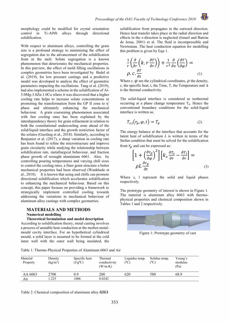
Proceedings of the OAU Faculty of Technology Conference 2019
353
morphology could be modified for crystal orientation control in Ti-AlNb alloys through directional solidification.
With respect to aluminum alloys, controlling the grain size is a profound strategy to minimizing the effect of segregation due to the advancement of the solidification front in the melt. Solute segregation is a known phenomenon that deteriorates the mechanical properties. In this purview, the effect of mold filling oscillations in complex geometries have been investigated by Bedel et al. (2019), for low pressure castings and a predictive model was developed to analyze the effect of geometric parameters impacting the oscillations. Tang et al. (2019), had also implemented a scheme in the solidification of Al-5.0Mg-3.0Zn-1.0Cu where it was discovered that a higher cooling rate helps to increase solute concentrations in promoting the transformation from the GP II zone to η′ phase and ultimately enhancing the mechanical behaviour. A grain coarsening phenomenon associated with fast cooling rates has been explained by the interdependency theory for grain refinement in relation to both the constitutional undercooling zone ahead of the solid/liquid interface and the growth restriction factor of the solutes (Guofang et al., 2018). Similarly, according to Benjunior et al. (2017), a sharp variation in cooling rate has been found to refine the microstructure and improve grain circularity while studying the relationship between solidification rate, metallurgical behaviour, and fraction phase growth of wrought aluminium 6061. Also, by controlling pouring temperatures and varying chill sizes to control the cooling rates, a finer grain structure a better mechanical properties had been observed (Wankhede et al., 2018). It is known that using end chills can promote directional solidification which accelerates solidification to enhancing the mechanical behaviour. Based on this concept, this paper focuses on providing a framework to strategically implement controlled cooling towards addressing the variations in mechanical behaviour of aluminum alloy castings with complex geometries.
MATERIALS AND METHODS Numerical modelling Theoretical formulation and model description According to solidification theory, metal casting involves a process of unstable heat conduction at the molten metal-mould cavity interface. For an hypothetical cylindrical mould, a solid layer is assumed to be formed at the cold inner wall with the outer wall being insulated, the
solidification front propagates in the outward direction. Hence heat transfer takes place in the radial direction and effects in the z-direction is neglected (Ismail and Batista de Jesus, 2001) et al. The fluid is incompressible and Newtonian. The heat conduction equation for modelling this problem is given by Equ 1.
1
𝑟(
𝜕
𝜕𝑟(𝑘. 𝑟
𝜕𝑇
𝜕𝑟)) +
1
𝑟2
𝜕
𝜕𝑥(
𝜕𝑇
𝜕𝜑) =
𝜌. 𝑐.𝜕𝑇
𝜕𝑡 (1)
Where r, 𝜑 are the cylindrical coordinates, 𝜌 the density, c, the specific heat, t, the Time, T, the Temperature and k is the thermal conductivity.
The solid-liquid interface is considered as isothermal occurring at a phase change temperature Tp. Hence the conventional boundary conditions for the solid-liquid interface is written as;
𝑇𝑠,𝑙(𝑟𝑝, 𝜑, 𝑡) = 𝑇𝑝 (2)
The energy balance at the interface that accounts for the latent heat of solidification L is written in terms of the Stefan condition that must be solved for the solidification front 𝑟𝑝 and can be expressed as:
[1 + (𝜕𝑟𝑝
𝜕𝜑)2
] [𝑘𝑠𝜕𝑇𝑠
𝜕𝑟−
𝜕𝑇𝑙
𝜕𝑟] =
𝜌𝐿𝜕𝑟𝑝
𝜕𝑡 (3)
Where s, l represent the solid and liquid phases respectively.
The prototype geometry of interest is shown in Figure 1. The material is aluminum alloy 6063 with thermo-physical properties and chemical composition shown in Tables 1 and 2 respectively.
Figure 1: Prototype geometry of cast
Table 1: Thermo-Physical Properties of Aluminum 6063 and Air
Material Property
Density (kg/m3)
Specific heat (J/g0C)
Thermal conductivity (W/m-K)
Liquidus temp. (0C)
Solidus temp. (0C)
Young’s modulus (Pa)
AA 6063 2700 0.9 200 620 580 68.9 Air 1.225 1006 0.0242
Table 2: Chemical composition of aluminum alloy 6063
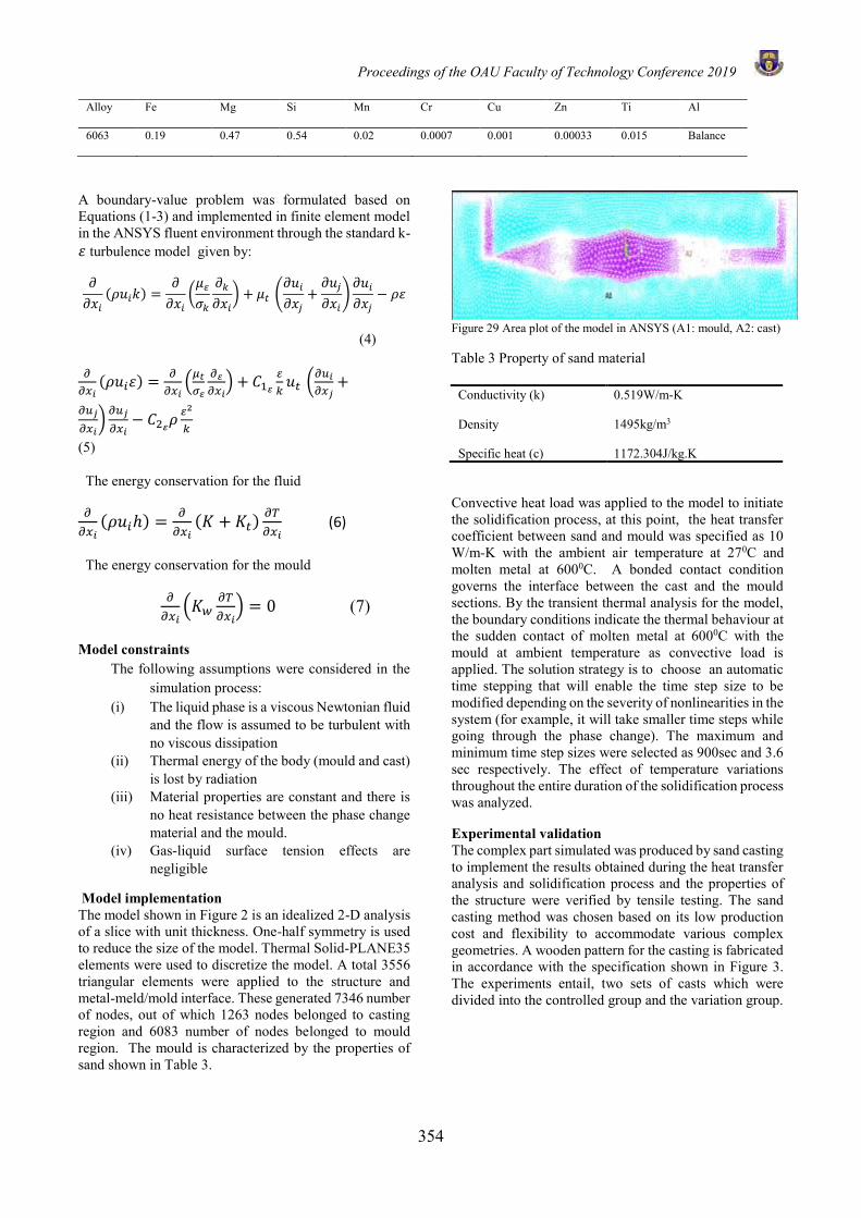
Proceedings of the OAU Faculty of Technology Conference 2019
354
Alloy Fe Mg Si Mn Cr Cu Zn Ti Al
6063 0.19 0.47 0.54 0.02 0.0007 0.001 0.00033 0.015 Balance
A boundary-value problem was formulated based on Equations (1-3) and implemented in finite element model in the ANSYS fluent environment through the standard k-𝜀 turbulence model given by:
𝜕
𝜕𝑥𝑖
(𝜌𝑢𝑖𝑘) =𝜕
𝜕𝑥𝑖
(𝜇𝜀
𝜎𝑘
𝜕𝑘
𝜕𝑥𝑖
) + 𝜇𝑡 (𝜕𝑢𝑖
𝜕𝑥𝑗
+𝜕𝑢𝑗
𝜕𝑥𝑖
)𝜕𝑢𝑖
𝜕𝑥𝑗
− 𝜌𝜀
(4)
𝜕
𝜕𝑥𝑖(𝜌𝑢𝑖𝜀) =
𝜕
𝜕𝑥𝑖(𝜇𝑡
𝜎𝜀
𝜕𝜀
𝜕𝑥𝑖) + 𝐶1𝜀
𝜀
𝑘𝑢𝑡 (
𝜕𝑢𝑖
𝜕𝑥𝑗+
𝜕𝑢𝑗
𝜕𝑥𝑖)
𝜕𝑢𝑗
𝜕𝑥𝑖− 𝐶2𝜀
𝜌𝜀2
𝑘
(5)
The energy conservation for the fluid
𝜕
𝜕𝑥𝑖(𝜌𝑢𝑖ℎ) =
𝜕
𝜕𝑥𝑖(𝐾 + 𝐾𝑡)
𝜕𝑇
𝜕𝑥𝑖 (6)
The energy conservation for the mould
𝜕
𝜕𝑥𝑖(𝐾𝑤
𝜕𝑇
𝜕𝑥𝑖) = 0 (7)
Model constraints The following assumptions were considered in the
simulation process: (i) The liquid phase is a viscous Newtonian fluid
and the flow is assumed to be turbulent with no viscous dissipation
(ii) Thermal energy of the body (mould and cast) is lost by radiation
(iii) Material properties are constant and there is no heat resistance between the phase change material and the mould.
(iv) Gas-liquid surface tension effects are negligible
Model implementation The model shown in Figure 2 is an idealized 2-D analysis of a slice with unit thickness. One-half symmetry is used to reduce the size of the model. Thermal Solid-PLANE35 elements were used to discretize the model. A total 3556 triangular elements were applied to the structure and metal-meld/mold interface. These generated 7346 number of nodes, out of which 1263 nodes belonged to casting region and 6083 number of nodes belonged to mould region. The mould is characterized by the properties of sand shown in Table 3.
Figure 29 Area plot of the model in ANSYS (A1: mould, A2: cast)
Table 3 Property of sand material
Convective heat load was applied to the model to initiate the solidification process, at this point, the heat transfer coefficient between sand and mould was specified as 10 W/m-K with the ambient air temperature at 270C and molten metal at 6000C. A bonded contact condition governs the interface between the cast and the mould sections. By the transient thermal analysis for the model, the boundary conditions indicate the thermal behaviour at the sudden contact of molten metal at 6000C with the mould at ambient temperature as convective load is applied. The solution strategy is to choose an automatic time stepping that will enable the time step size to be modified depending on the severity of nonlinearities in the system (for example, it will take smaller time steps while going through the phase change). The maximum and minimum time step sizes were selected as 900sec and 3.6 sec respectively. The effect of temperature variations throughout the entire duration of the solidification process was analyzed.
Experimental validation The complex part simulated was produced by sand casting to implement the results obtained during the heat transfer analysis and solidification process and the properties of the structure were verified by tensile testing. The sand casting method was chosen based on its low production cost and flexibility to accommodate various complex geometries. A wooden pattern for the casting is fabricated in accordance with the specification shown in Figure 3. The experiments entail, two sets of casts which were divided into the controlled group and the variation group.
Conductivity (k) 0.519W/m-K
Density 1495kg/m3
Specific heat (c) 1172.304J/kg.K
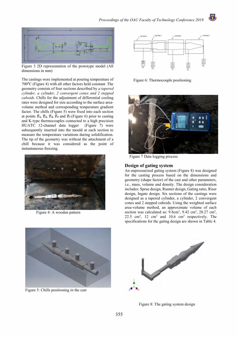
Proceedings of the OAU Faculty of Technology Conference 2019
355
Figure 3 2D representation of the prototype model (All dimensions in mm)
The castings were implemented at pouring temperature of 7000C (Figure 4) with all other factors held constant. The geometry consists of four sections described by a tapered cylinder, a cylinder, 2 convergent cones and 2 stepped cuboids. Chills for the adjustment of differential cooling rates were designed for size according to the surface area-volume method and corresponding temperature gradient factor. The chills (Figure 5) were fixed into each section at points T1, T2, T3, T4 and T5
(Figure 6) prior to casting and K-type thermocouples connected to a high precision HUATC 12-channel data logger (Figure 7) were subsequently inserted into the mould at each section to measure the temperature variations during solidification. The tip of the geometry was without the attachment of a chill because it was considered as the point of instantaneous freezing.
Figure 4: A wooden pattern
Figure 5: Chills positioning in the cast
Figure 6: Thermocouple positioning
Figure 7 Data logging process
Design of gating system An unpressurized gating system (Figure 8) was designed for the casting process based on the dimensions and geometry (shape factor) of the cast and other parameters, i.e., mass, volume and density. The design consideration includes: Sprue design, Runner design, Gating ratio, Riser design, Ingate design. Six sections of the castings were designed as a tapered cylinder, a cylinder, 2 convergent cones and 2 stepped cuboids. Using the weighted surface area-volume method, an approximate volume of each section was calculated as: 9.8cm3, 9.42 cm3, 28.27 cm3, 22.5 cm3, 12 cm3 and 10.6 cm3 respectively. The specifications for the gating design are shown in Table 4.
Figure 8: The gating system design
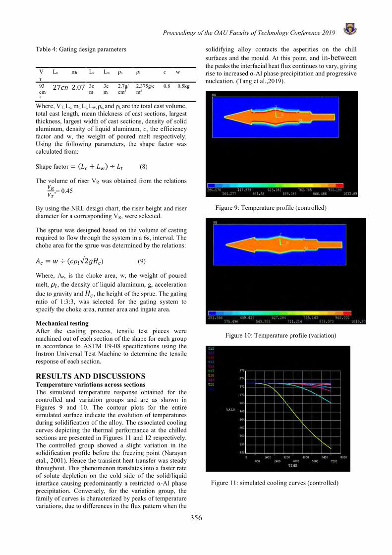
Proceedings of the OAU Faculty of Technology Conference 2019
356
Table 4: Gating design parameters
Where, VT, Lc, mt, Lt, Lw, ρs, and ρl, are the total cast volume, total cast length, mean thickness of cast sections, largest thickness, largest width of cast sections, density of solid aluminum, density of liquid aluminum, c, the efficiency factor and w, the weight of poured melt respectively. Using the following parameters, the shape factor was calculated from:
Shape factor = (𝐿𝑐 + 𝐿𝑤) ÷ 𝐿𝑡 (8)
The volume of riser VR was obtained from the relations 𝑉𝑅
𝑉𝑇,= 0.45
By using the NRL design chart, the riser height and riser diameter for a corresponding VR, were selected.
The sprue was designed based on the volume of casting required to flow through the system in a 6s, interval. The chohe area for the sprue was determined by the relations:
𝐴𝑐 = 𝑤 ÷ (𝑐𝜌𝑙√2𝑔𝐻𝑐) (9)
Where, Ac, is the choke area, w, the weight of poured melt, 𝜌𝑙 , the density of liquid aluminum, g, acceleration due to gravity and 𝐻𝑐, the height of the sprue. The gating ratio of 1:3:3, was selected for the gating system to specify the choke area, runner area and ingate area.
Mechanical testing After the casting process, tensile test pieces were
machined out of each section of the shape for each group in accordance to ASTM E9-08 specifications using the Instron Universal Test Machine to determine the tensile response of each section.
RESULTS AND DISCUSSIONS Temperature variations across sections The simulated temperature response obtained for the controlled and variation groups and are as shown in Figures 9 and 10. The contour plots for the entire simulated surface indicate the evolution of temperatures during solidification of the alloy. The associated cooling curves depicting the thermal performance at the chilled sections are presented in Figures 11 and 12 respectively. The controlled group showed a slight variation in the solidification profile before the freezing point (Narayan etal., 2001). Hence the transient heat transfer was steady throughout. This phenomenon translates into a faster rate of solute depletion on the cold side of the solid/liquid interface causing predominantly a restricted α-Al phase precipitation. Conversely, for the variation group, the family of curves is characterized by peaks of temperature variations, due to differences in the flux pattern when the
solidifying alloy contacts the asperities on the chill surfaces and the mould. At this point, and in-between the peaks the interfacial heat flux continues to vary, giving rise to increased α-Al phase precipitation and progressive nucleation. (Tang et al.,2019).
Figure 9: Temperature profile (controlled)
Figure 10: Temperature profile (variation)
Figure 11: simulated cooling curves (controlled)
VT
Lc mt Lt Lw ρs ρl c w
93 cm3
27𝑐𝑚3 2.07𝑐𝑚 3cm
3cm
2.7g/cm3
2.375g/cm3
0.8 0.5kg
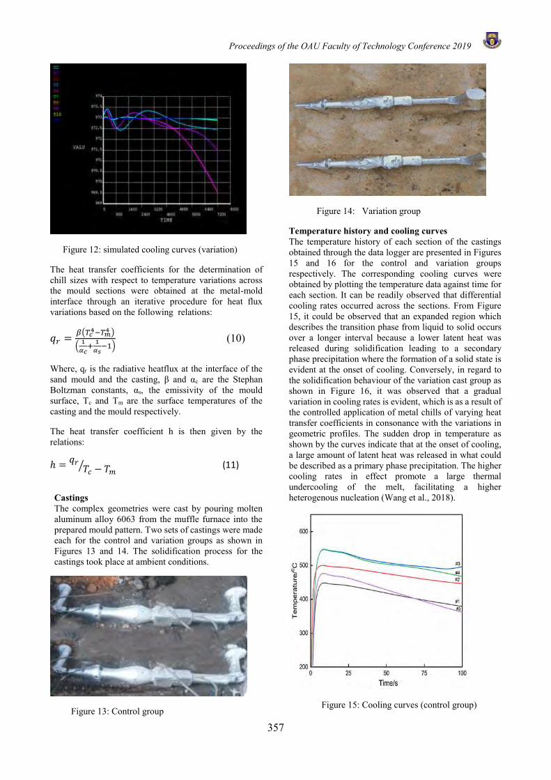
Proceedings of the OAU Faculty of Technology Conference 2019
357
Figure 12: simulated cooling curves (variation)
The heat transfer coefficients for the determination of chill sizes with respect to temperature variations across the mould sections were obtained at the metal-mold interface through an iterative procedure for heat flux variations based on the following relations:
𝑞𝑟 =𝛽(𝑇𝑐
4−𝑇𝑚4 )
(1
𝛼𝑐+
1
𝛼𝑠−1)
(10)
Where, qr is the radiative heatflux at the interface of the sand mould and the casting, β and αc are the Stephan Boltzman constants, αs, the emissivity of the mould surface, Tc and Tm are the surface temperatures of the casting and the mould respectively.
The heat transfer coefficient h is then given by the relations:
ℎ =𝑞𝑟
𝑇𝑐 − 𝑇𝑚⁄ (11)
Castings The complex geometries were cast by pouring molten aluminum alloy 6063 from the muffle furnace into the prepared mould pattern. Two sets of castings were made each for the control and variation groups as shown in Figures 13 and 14. The solidification process for the castings took place at ambient conditions.
Figure 13: Control group
Figure 14: Variation group
Temperature history and cooling curves The temperature history of each section of the castings obtained through the data logger are presented in Figures 15 and 16 for the control and variation groups respectively. The corresponding cooling curves were obtained by plotting the temperature data against time for each section. It can be readily observed that differential cooling rates occurred across the sections. From Figure 15, it could be observed that an expanded region which describes the transition phase from liquid to solid occurs over a longer interval because a lower latent heat was released during solidification leading to a secondary phase precipitation where the formation of a solid state is evident at the onset of cooling. Conversely, in regard to the solidification behaviour of the variation cast group as shown in Figure 16, it was observed that a gradual variation in cooling rates is evident, which is as a result of the controlled application of metal chills of varying heat transfer coefficients in consonance with the variations in geometric profiles. The sudden drop in temperature as shown by the curves indicate that at the onset of cooling, a large amount of latent heat was released in what could be described as a primary phase precipitation. The higher cooling rates in effect promote a large thermal undercooling of the melt, facilitating a higher heterogenous nucleation (Wang et al., 2018).
Figure 15: Cooling curves (control group)
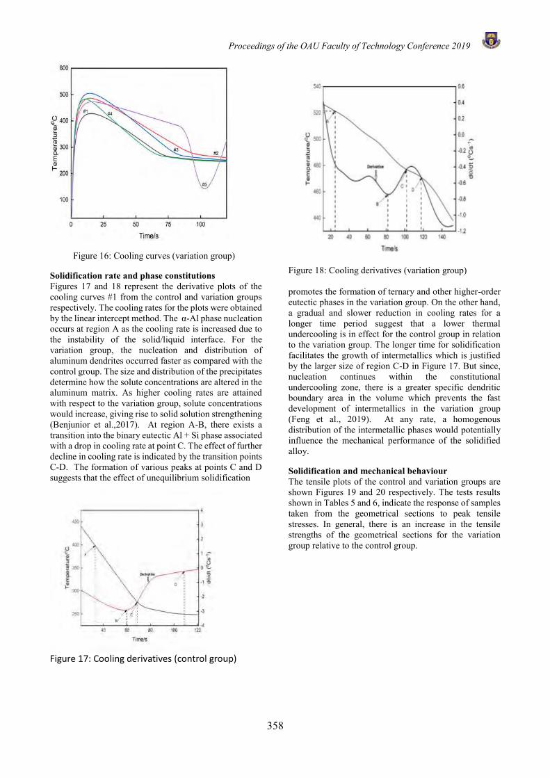
Proceedings of the OAU Faculty of Technology Conference 2019
358
Figure 16: Cooling curves (variation group)
Solidification rate and phase constitutions Figures 17 and 18 represent the derivative plots of the cooling curves #1 from the control and variation groups respectively. The cooling rates for the plots were obtained by the linear intercept method. The α-Al phase nucleation occurs at region A as the cooling rate is increased due to the instability of the solid/liquid interface. For the variation group, the nucleation and distribution of aluminum dendrites occurred faster as compared with the control group. The size and distribution of the precipitates determine how the solute concentrations are altered in the aluminum matrix. As higher cooling rates are attained with respect to the variation group, solute concentrations would increase, giving rise to solid solution strengthening (Benjunior et al.,2017). At region A-B, there exists a transition into the binary eutectic Al + Si phase associated with a drop in cooling rate at point C. The effect of further decline in cooling rate is indicated by the transition points C-D. The formation of various peaks at points C and D suggests that the effect of unequilibrium solidification
Figure 17: Cooling derivatives (control group)
Figure 18: Cooling derivatives (variation group) promotes the formation of ternary and other higher-order eutectic phases in the variation group. On the other hand, a gradual and slower reduction in cooling rates for a longer time period suggest that a lower thermal undercooling is in effect for the control group in relation to the variation group. The longer time for solidification facilitates the growth of intermetallics which is justified by the larger size of region C-D in Figure 17. But since, nucleation continues within the constitutional undercooling zone, there is a greater specific dendritic boundary area in the volume which prevents the fast development of intermetallics in the variation group (Feng et al., 2019). At any rate, a homogenous distribution of the intermetallic phases would potentially influence the mechanical performance of the solidified alloy.
Solidification and mechanical behaviour The tensile plots of the control and variation groups are shown Figures 19 and 20 respectively. The tests results shown in Tables 5 and 6, indicate the response of samples taken from the geometrical sections to peak tensile stresses. In general, there is an increase in the tensile strengths of the geometrical sections for the variation group relative to the control group.
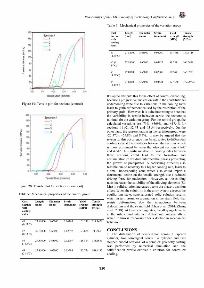
Proceedings of the OAU Faculty of Technology Conference 2019
359
Figure 19: Tensile plot for sections (control)
Figure 20: Tensile plot for sections (variationl) Table 5: Mechanical properties of the control group
Cast Section with cooling rates
Length (mm)
Diameter (mm)
Strain (mm/mm)
Yield srength (MPa)
Tensile strength (MPa)
#1 (0.570C)
27.81000 5.65000 0.04765 101.336 114.1428
#2 (0.330C)
27.81000 5.65000 0.02697 17.9878 30.5661
#3 (1.680C)
27.81000 5.65000 0.02097 116.884 143.3633
#4 (2.810C)
27.81000 5.65000 0.03986 112.776 168.4137
Table 6: Mechanical properties of the variation group
Cast Section with cooling rates
Length (mm)
Diameter (mm)
Strain (mm/mm)
Yield strength (MPa)
Tensile strength (MPa)
#1 (2.710C)
27.81000 5.65000 0.03269 107.458 137.6748
#2 (1. 440C)
27.81000 5.65000 0.03927 88.781 106.5998
#3 (3.690C)
27.81000 5.65000 0.02908 122.471 166.0909
#4 (3.440C)
27.81000 5.65000 0.04824 127.338 179.90775
It’s apt to attribute this to the effect of controlled cooling, because a progressive nucleation within the constitutional undercooling zone due to variations in the cooling rates leads to grain refinement caused by the restriction of the primary grain. However, it is quite interesting to note that the variability in tensile behavior across the sections is minimal for the variation group. For the control group, the calculated variations are -73%, +369%, and +17.4% for sections #1-#2, #2-#3 and #3-#4 respectively. On the other hand, the representations in the variation group were -22.57%, +55.8% and 8.3%. It may be argued that the reason for this occurrence may be attributed to differential cooling rates at the interfaces between the sections which is more prominent between the adjacent sections #1-#2 and #2-#3. A significant drop in cooling rates between these sections could lead to the formation and accumulation of residual intermetallic phases preventing the growth of precipitates. A coarsening effect is also feasible due to recovery to a higher cooling rate, leads to a small undercooling zone which also could impart a detrimental action on the tensile strength due a reduced driving force for nucleation. However, as the cooling rates increase, the solubility of the alloying elements (Si, Mn) in solid solution increases due to the phase-transition effect. When the solubility in the alloy system exceeds the equilibrium state, supersaturated solid solution results, which in turn promotes a variation in the strain field that resists deformation due the interactions between dislocations and the strain field (Chen et al., 2014; Zhang et al., 2018). At lower cooling rates, the alloying elements at the solid-liquid interface diffuse into intermetallics, which in turn is responsible for a decline in mechanical behaviour.
CONCLUSIONS 1. The distribution of temperature across a tapered cylinder, two convergent cones , a cylinder and two stepped cuboid sections of a complex geometry casting was performed by numerical simulation and the solidification profile evolved a criterion for controlled cooling.
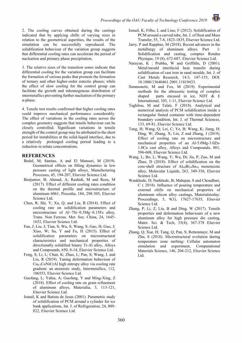
Proceedings of the OAU Faculty of Technology Conference 2019
360
2. The cooling curves obtained during the castings indicated that by applying chills of varying sizes in relation to the geometrical asperities, the results of the simulation can be successfully reproduced. The solidification behaviour of the variation group suggests that differential cooling rates can accelerate the period of nucleation and primary phase precipitation.
3. The relative sizes of the transition zones indicate that differential cooling for the variation group can facilitate the formation of various peaks that promote the formation of ternary and other higher-order eutectic phases; while the effect of slow cooling for the control group can facilitate the growth and inhomogenous distribution of intermetallics preventing further nucleation of the primary α-phase.
4. Tensile test results confirmed that higher cooling rates could improve mechanical performance considerably. The effect of variations in the cooling rates across the complex geometry suggests that tensile behaviour can be closely controlled. Significant variations in tensile strength of the control group may be attributed to the short period for instabilities at the solid-liquid interface, due to a relatively prolonged cooling period leading to a reduction in solute concentrations.
REFERENCES Bedel, M; Sanitas, A and El Mansori, M (2019).
Geometrical effects on filling dynamics in low pressure casting of light alloys, Manufacturing Processes, 45, 194-207, Elsevier Science Ltd.
Benjunior, B; Ahmad, A; Rashidi, M and Reza, M (2017). Effect of different cooling rates condition on the thermal profile and microstructure of aluminum 6061, Procedia, 184, 298-305, Elsevier Science Ltd.
Chen, R; Shi, Y; Xu, Q; and Liu, B (2014). Effect of cooling rate on solidification parameters and microstructure of Al−7Si−0.3Mg−0.15Fe alloy, Trans. Non Ferrous. Met. Soc. China, 24, 1645-1652, Elsevier Science Ltd.
Fan, J; Liu, J; Tian, S; Wu, S; Wang, S; Gao, H; Guo, J; Xiao, W; Su, Y and Fu, H (2015). Effect of solidification parameters on microstructural characteristics and mechanical properties of directionally solidified binary Ti-Al alloy, Alloys and Compounds, 650, 8-14, Elsevier Science Ltd.
Feng, S; Li, L; Chan, K; Zhao, L; Pan, S; Wang, L and Liu, R (2019). Tuning deformation behaviour of Cu0.5CoNiCrAl high entropy alloy via cooling rate gradient: an atomistic study, Intermetallics, 112, 106553, Elsevier Science Ltd.
Guofang, L; Yahia, A; Guofang, Y and Ming-Xing, Z (2018). Effect of cooling rate on grain refinement of aluminum alloys, Materialia, 3, 113-121, Elsevier Science Ltd.
Ismail, K and Batista de Jesus (2001). Parametric study of solidification of PCM around a cylinder for ice bank applications, Int. J. of Refrigeration, 24, 809-822, Elsevier Science Ltd.
Ismail, K; Filho, L and Lino, F (2012). Solidification of PCM around a curved tube, Int. J. of Heat and Mass Transfer, 55, 7-8, 1823-1835, Elsevier Science Ltd.
Jarry, P and Rapphaz, M (2018). Recent advances in the metallurgy of aluminum alloys. Part 1: Solidification and casting, comptes Rendus Physique, 19 (8), 672-687, Elsevier Science Ltd.
Narayan, K ; Prabhu, W and Griffiths, D (2001). Metal/mould interfacial heat transfer during solidification of cast iron in sand moulds, Int. J. of Cast Metals Research, 14:3, 147-155, DOI: 10.1080/13640461.2001.11819433.
Simmonetti, M and Fox, M (2019). Experimental methods for the ultrasonic testing of complex shaped parts encased in ice, NDT & E International, 103, 1-11, Elsevier Science Ltd.
Taghilou, M and Talati, F (2018). Analytical and numerical analysis of PCM solidification inside a rectangular finned container with time-dependent boundary condition, Int. J. of Thermal Sciences, 133, 69-81, Elsevier Science Ltd.
Tang, H; Wang, Q; Lei, C; Ye, B; Wang, K; Jiang, H; Ding, W; Zhang, X; Lin, Z and Zhang, J (2019). Effect of cooling rate on microstructure and mechanical properties of an Al-5.0Mg-3.0Zn-1.0Cu cast alloy, Alloys and Compounds, 801, 596-608, Elsevier Science Ltd.
Wang, L; Bo, L; Wang, Y; Wu, Di; Jia, P; Zuo, M and Zhao, D (2018). Effect of solidification on the core-shell structure of Al60Bi24Sn16 monotecnic alloy, Molecular Liquids, 263, 349-356, Elsevier Science Ltd.
Wankhede, D; Narkhede, B; Mahajan, S and Choudhari, C ( 2018). Influence of pouring temperature and external chills on mechanical properties of aluminum silicon alloy castings, Materialstoday: Proceedings, 5, 9(3), 17627-17635, Elsevier Science Ltd.
Zhang, P; Li, Z; Liu, B and Ding, W (2017). Tensile properties and deformation behaviours of a new aluminum alloy for high pressure die casting, Mater. Sci. & Tech, 33(4), 367-378 Elsevier Science Ltd.
Zhang, Q; Xue, H; Tang, Q; Pan, S; Rettenmayr, M and Zhu, S (2018). Microstructural evolution during temperature zone melting: Cellular automaton simulation and experiment, Computational Materials Science, 146, 204-212, Elsevier Science Ltd.
Proceedings of the OAU Faculty of Technology Conference 2019
361
UTILISATION OF PHOSPHORIC ACID TO IMPROVE THE PROPERTIES OF ADOBE BRICKS FOR LOW-COST HOUSING
A. O. Mohammed*, A. L. Ayodele, A. B. Fajobi, A. A. Akindahunsi and A. M. Olajumoke. Department of Civil Engineering,
Obafemi Awolowo University, Nigeria.
*Email of Corresponding Author: [email protected]
ABSTRACT This study investigates the use of phosphoric acid (H3PO4) in stabilising lateritic soil to produce adobe bricks of improved engineering properties. The index properties such as Atterberg’s limit, percentage fines content, moisture-density relationship and inherent elements in the lateritic soil were determined. Various percentages up to 8% at 2% interval of 1 Molar concentration of H3PO4 were mixed with the lateritic soil for stabilisation purpose. Hollow adobe bricks were produced from the different mix ratios. Control adobe bricks were also produced from 5% cement stabilised lateritic soil based on the recommended maximum cement stabilisation level for lateritic soil by the Nigerian Building and Road Research Institute (NBRRI). The bricks were cured for 7, 14, 21 and 28 days under ambient air condition. The compressive strength (fc) and modulus of rupture (fr) of the bricks were determined at each of the curing days. After 28 days of curing, the maximum fc of 1.7 N/mm2 and 2.0 N/mm2 were obtained at 6 % stabilisation with 1M H3PO4 and 5% cement stabilised bricks, respectively. Their maximum fr are 0.29 N/mm2 and 0.47 N/mm2, respectively. The compressive strength obtained for H3PO4 stabilised hollow adobe bricks satisfies the minimum strength requirement of 1.65 N/mm2 for adobe bricks as recommended by NBRRI. It can therefore be concluded that diluted phosphoric acid can be used as an alternative to cement for stabilising adobe bricks for construction of low-cost housing. Keywords: Phosphoric acid, Lateritic soil, Adobe bricks, Compressive strength, Modulus of rupture INTRODUCTION In recent times, there has been a consciousness to reduce direct and indirect energy produced from the building industry in order to lessen the harmful effects on the ecosystem. The present use of construction materials has affected the ecosystem negatively and limited technical developments in the building industry (Benghida, 2015). In order to remedy this, it is encouraged that the use of building construction materials should be conservative, recycled and reused (Benghida, 2015). Adobe bricks are building materials that are eco-friendly but just like any other building material, it has its strengths and weaknesses (Benghida, 2015). Adobe is one of the oldest and most widely used building construction materials (Sahu and Singh, 2017). It has been used for thousands of years for the construction of buildings and other structures. The word “Adobe” is used generally to describe different earth materials that are used in building construction and the method in which they are used. Mud plastering material, puddled earth material and rammed earth construction can be identified as adobe (Smith and Austin, 1989). Generally, structures are considered to be adobe when the principal building material is soil or mud (Sahu and Singh, 2017). Earth materials for the production of adobe bricks are abundantly available and affordable at a low cost. Adobe bricks can be easily produced by mixing earth material with water, placing and compacting the resulting mixture in the moulds. Then, the mixture in the mould is left to dry in the open air away from the sun (Sahu and Singh, 2017). Construction of buildings with adobe bricks offers
thermal comfort in hot weather conditions and has low levels of sound transmission through walls (Bahobail, 2012). The walls store the heat and reduce the rate at which heat is transferred into the building (Begum, et al., 2014). Adobe bricks are also durable, non-toxic, fireproof and economic(Benghida, 2015). The production of adobe bricks is easy because the process does not require specialized skills. It depends mainly on human labour and creativity (Bahobail, 2014). Adobe bricks offer flexibility in the design and construction of buildings because they can be easily cut, shaped and subjected to openings for building’s services (Sahu and Singh, 2017). The major weakness of adobe bricks is when they are soaked in water and under rain (Sahu and Singh, 2017). Studies have been carried out to improve the physical properties and performance of adobe bricks using different additives. Some of such physical properties include compressive strength, modulus of rupture, density, porosity, water absorption, depth of penetration, abrasion resistance and hardness. Lateritic soils for the production of adobe bricks or laterised bricks have been stabilized with ordinary Portland cement (Begum, et al., 2014), coconut hush ash (Olajumoke, et al., 2011), natural rubber latex (Wahabi, 2017), recycled sugarcane fibre waste (Bock-hyeng, et al., 2016), sawdust and egg shell ash (Ayodele, et al., 2019), and other stabilizers. According to Begum, et al., (2014) a compressive strength of 6.68 N/mm2 was achieved at 5 % stabilisation with natural rubber latex and cement. Olajumoke, et al., (2011) stabilised lateritic soils from three locations with up to 6% coconut shell ash (CSA) and
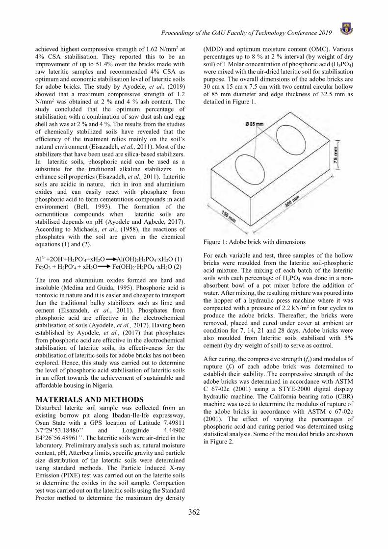
Proceedings of the OAU Faculty of Technology Conference 2019
362
achieved highest compressive strength of 1.62 N/mm2 at 4% CSA stabilisation. They reported this to be an improvement of up to 51.4% over the bricks made with raw lateritic samples and recommended 4% CSA as optimum and economic stabilisation level of lateritic soils for adobe bricks. The study by Ayodele, et al., (2019) showed that a maximum compressive strength of 1.2 N/mm2 was obtained at 2 % and 4 % ash content. The study concluded that the optimum percentage of stabilisation with a combination of saw dust ash and egg shell ash was at 2 % and 4 %. The results from the studies of chemically stabilized soils have revealed that the efficiency of the treatment relies mainly on the soil’s natural environment (Eisazadeh, et al., 2011). Most of the stabilizers that have been used are silica-based stabilizers. In lateritic soils, phosphoric acid can be used as a substitute for the traditional alkaline stabilizers to enhance soil properties (Eisazadeh, et al., 2011). Lateritic soils are acidic in nature, rich in iron and aluminium oxides and can easily react with phosphate from phosphoric acid to form cementitious compounds in acid environment (Bell, 1993). The formation of the cementitious compounds when lateritic soils are stabilised depends on pH (Ayodele and Agbede, 2017). According to Michaels, et al., (1958), the reactions of phosphates with the soil are given in the chemical equations (1) and (2). Al3++2OH-+H2PO-
4+xH2O Al(OH)2H2PO4·xH2O (1) Fe2O3 + H2PO-
4 + xH2O Fe(OH)2·H2PO4 ·xH2O (2) The iron and aluminium oxides formed are hard and insoluble (Medina and Guida, 1995). Phosphoric acid is nontoxic in nature and it is easier and cheaper to transport than the traditional bulky stabilizers such as lime and cement (Eisazadeh, et al., 2011). Phosphates from phosphoric acid are effective in the electrochemical stabilisation of soils (Ayodele, et al., 2017). Having been established by Ayodele, et al., (2017) that phosphates from phosphoric acid are effective in the electrochemical stabilisation of lateritic soils, its effectiveness for the stabilisation of lateritic soils for adobe bricks has not been explored. Hence, this study was carried out to determine the level of phosphoric acid stabilisation of lateritic soils in an effort towards the achievement of sustainable and affordable housing in Nigeria. MATERIALS AND METHODS Disturbed laterite soil sample was collected from an existing borrow pit along Ibadan-Ile-Ife expressway, Osun State with a GPS location of Latitude 7.49811 N7°29’53.18486’’ and Longitude 4.44902 E4°26’56.48961’’. The lateritic soils were air-dried in the laboratory. Preliminary analysis such as; natural moisture content, pH, Atterberg limits, specific gravity and particle size distribution of the lateritic soils were determined using standard methods. The Particle Induced X-ray Emission (PIXE) test was carried out on the laterite soils to determine the oxides in the soil sample. Compaction test was carried out on the lateritic soils using the Standard Proctor method to determine the maximum dry density
(MDD) and optimum moisture content (OMC). Various percentages up to 8 % at 2 % interval (by weight of dry soil) of 1 Molar concentration of phosphoric acid (H3PO4) were mixed with the air-dried lateritic soil for stabilisation purpose. The overall dimensions of the adobe bricks are 30 cm x 15 cm x 7.5 cm with two central circular hollow of 85 mm diameter and edge thickness of 32.5 mm as detailed in Figure 1.
Figure 1: Adobe brick with dimensions For each variable and test, three samples of the hollow bricks were moulded from the lateritic soil-phosphoric acid mixture. The mixing of each batch of the lateritic soils with each percentage of H3PO4 was done in a non-absorbent bowl of a pot mixer before the addition of water. After mixing, the resulting mixture was poured into the hopper of a hydraulic press machine where it was compacted with a pressure of 2.2 kN/m2 in four cycles to produce the adobe bricks. Thereafter, the bricks were removed, placed and cured under cover at ambient air condition for 7, 14, 21 and 28 days. Adobe bricks were also moulded from lateritic soils stabilised with 5% cement (by dry weight of soil) to serve as control. After curing, the compressive strength (fc) and modulus of rupture (fr) of each adobe brick was determined to establish their stability. The compressive strength of the adobe bricks was determined in accordance with ASTM C 67-02c (2001) using a STYE-2000 digital display hydraulic machine. The California bearing ratio (CBR) machine was used to determine the modulus of rupture of the adobe bricks in accordance with ASTM c 67-02c (2001). The effect of varying the percentages of phosphoric acid and curing period was determined using statistical analysis. Some of the moulded bricks are shown in Figure 2.
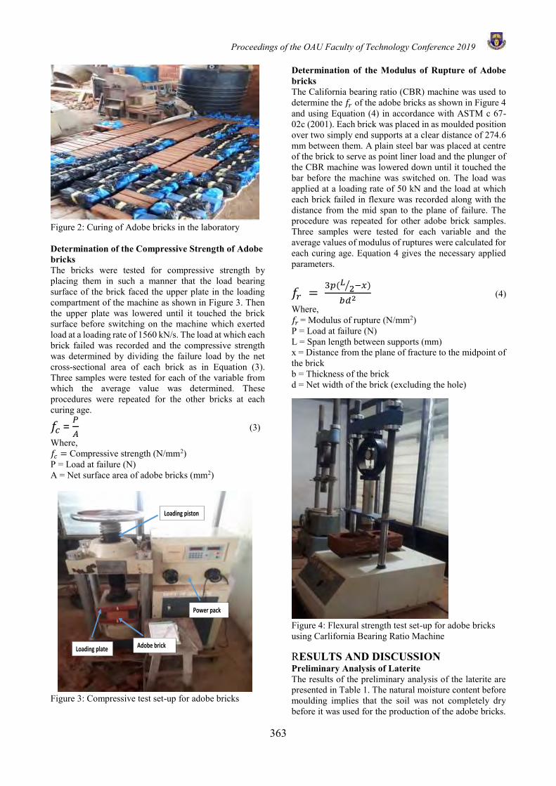
Proceedings of the OAU Faculty of Technology Conference 2019
363
Figure 2: Curing of Adobe bricks in the laboratory Determination of the Compressive Strength of Adobe bricks The bricks were tested for compressive strength by placing them in such a manner that the load bearing surface of the brick faced the upper plate in the loading compartment of the machine as shown in Figure 3. Then the upper plate was lowered until it touched the brick surface before switching on the machine which exerted load at a loading rate of 1560 kN/s. The load at which each brick failed was recorded and the compressive strength was determined by dividing the failure load by the net cross-sectional area of each brick as in Equation (3). Three samples were tested for each of the variable from which the average value was determined. These procedures were repeated for the other bricks at each curing age.
𝑓𝑐 = 𝑃
𝐴 (3)
Where, 𝑓𝑐 = Compressive strength (N/mm2) P = Load at failure (N) A = Net surface area of adobe bricks (mm2)
Figure 3: Compressive test set-up for adobe bricks
Determination of the Modulus of Rupture of Adobe bricks The California bearing ratio (CBR) machine was used to determine the 𝑓𝑟 of the adobe bricks as shown in Figure 4 and using Equation (4) in accordance with ASTM c 67-02c (2001). Each brick was placed in as moulded position over two simply end supports at a clear distance of 274.6 mm between them. A plain steel bar was placed at centre of the brick to serve as point liner load and the plunger of the CBR machine was lowered down until it touched the bar before the machine was switched on. The load was applied at a loading rate of 50 kN and the load at which each brick failed in flexure was recorded along with the distance from the mid span to the plane of failure. The procedure was repeated for other adobe brick samples. Three samples were tested for each variable and the average values of modulus of ruptures were calculated for each curing age. Equation 4 gives the necessary applied parameters.
𝑓𝑟 = 3𝑝(𝐿 2⁄ −𝑥)
𝑏𝑑2 (4)
Where, 𝑓𝑟 = Modulus of rupture (N/mm2) P = Load at failure (N) L = Span length between supports (mm) x = Distance from the plane of fracture to the midpoint of the brick b = Thickness of the brick d = Net width of the brick (excluding the hole)
Figure 4: Flexural strength test set-up for adobe bricks using Carlifornia Bearing Ratio Machine RESULTS AND DISCUSSION Preliminary Analysis of Laterite The results of the preliminary analysis of the laterite are presented in Table 1. The natural moisture content before moulding implies that the soil was not completely dry before it was used for the production of the adobe bricks.
Loading piston
Loading plate
Power pack
Adobe brick
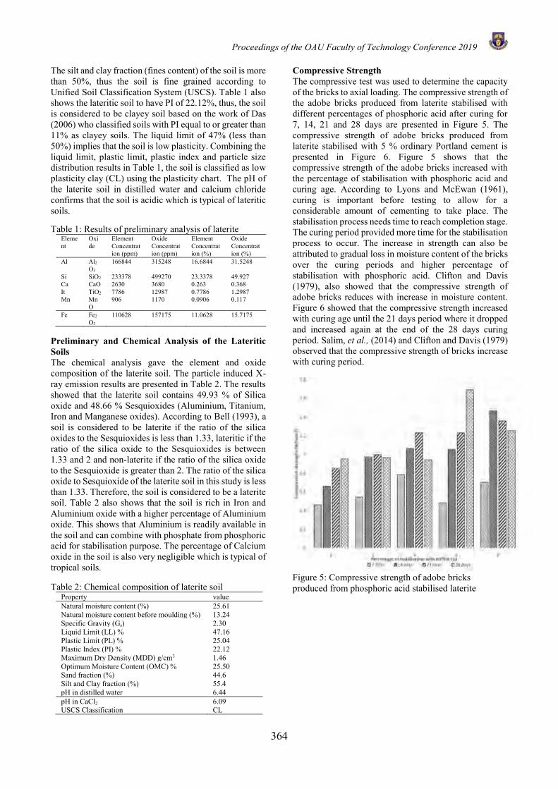
Proceedings of the OAU Faculty of Technology Conference 2019
364
The silt and clay fraction (fines content) of the soil is more than 50%, thus the soil is fine grained according to Unified Soil Classification System (USCS). Table 1 also shows the lateritic soil to have PI of 22.12%, thus, the soil is considered to be clayey soil based on the work of Das (2006) who classified soils with PI equal to or greater than 11% as clayey soils. The liquid limit of 47% (less than 50%) implies that the soil is low plasticity. Combining the liquid limit, plastic limit, plastic index and particle size distribution results in Table 1, the soil is classified as low plasticity clay (CL) using the plasticity chart. The pH of the laterite soil in distilled water and calcium chloride confirms that the soil is acidic which is typical of lateritic soils. Table 1: Results of preliminary analysis of laterite
Element
Oxide
Element Concentration (ppm)
Oxide Concentration (ppm)
Element Concentration (%)
Oxide Concentration (%)
Al Al2O3
166844 315248 16.6844 31.5248
Si SiO2 233378 499270 23.3378 49.927 Ca CaO 2630 3680 0.263 0.368 It TiO2 7786 12987 0.7786 1.2987 Mn Mn
O 906 1170 0.0906 0.117
Fe Fe2
O3 110628 157175 11.0628 15.7175
Preliminary and Chemical Analysis of the Lateritic Soils The chemical analysis gave the element and oxide composition of the laterite soil. The particle induced X-ray emission results are presented in Table 2. The results showed that the laterite soil contains 49.93 % of Silica oxide and 48.66 % Sesquioxides (Aluminium, Titanium, Iron and Manganese oxides). According to Bell (1993), a soil is considered to be laterite if the ratio of the silica oxides to the Sesquioxides is less than 1.33, lateritic if the ratio of the silica oxide to the Sesquioxides is between 1.33 and 2 and non-laterite if the ratio of the silica oxide to the Sesquioxide is greater than 2. The ratio of the silica oxide to Sesquioxide of the laterite soil in this study is less than 1.33. Therefore, the soil is considered to be a laterite soil. Table 2 also shows that the soil is rich in Iron and Aluminium oxide with a higher percentage of Aluminium oxide. This shows that Aluminium is readily available in the soil and can combine with phosphate from phosphoric acid for stabilisation purpose. The percentage of Calcium oxide in the soil is also very negligible which is typical of tropical soils. Table 2: Chemical composition of laterite soil
Property value Natural moisture content (%) 25.61 Natural moisture content before moulding (%) 13.24 Specific Gravity (Gs) 2.30 Liquid Limit (LL) % 47.16 Plastic Limit (PL) % 25.04 Plastic Index (PI) % 22.12 Maximum Dry Density (MDD) g/cm3 1.46 Optimum Moisture Content (OMC) % 25.50 Sand fraction (%) 44.6 Silt and Clay fraction (%) 55.4 pH in distilled water 6.44 pH in CaCl2 USCS Classification
6.09 CL
Compressive Strength The compressive test was used to determine the capacity of the bricks to axial loading. The compressive strength of the adobe bricks produced from laterite stabilised with different percentages of phosphoric acid after curing for 7, 14, 21 and 28 days are presented in Figure 5. The compressive strength of adobe bricks produced from laterite stabilised with 5 % ordinary Portland cement is presented in Figure 6. Figure 5 shows that the compressive strength of the adobe bricks increased with the percentage of stabilisation with phosphoric acid and curing age. According to Lyons and McEwan (1961), curing is important before testing to allow for a considerable amount of cementing to take place. The stabilisation process needs time to reach completion stage. The curing period provided more time for the stabilisation process to occur. The increase in strength can also be attributed to gradual loss in moisture content of the bricks over the curing periods and higher percentage of stabilisation with phosphoric acid. Clifton and Davis (1979), also showed that the compressive strength of adobe bricks reduces with increase in moisture content. Figure 6 showed that the compressive strength increased with curing age until the 21 days period where it dropped and increased again at the end of the 28 days curing period. Salim, et al., (2014) and Clifton and Davis (1979) observed that the compressive strength of bricks increase with curing period.
Figure 5: Compressive strength of adobe bricks produced from phosphoric acid stabilised laterite
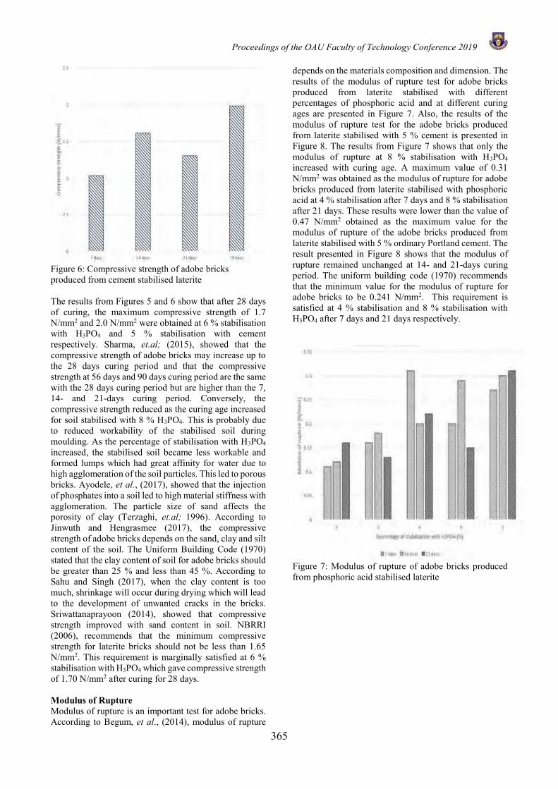
Proceedings of the OAU Faculty of Technology Conference 2019
365
Figure 6: Compressive strength of adobe bricks produced from cement stabilised laterite The results from Figures 5 and 6 show that after 28 days of curing, the maximum compressive strength of 1.7 N/mm2 and 2.0 N/mm2 were obtained at 6 % stabilisation with H3PO4 and 5 % stabilisation with cement respectively. Sharma, et.al; (2015), showed that the compressive strength of adobe bricks may increase up to the 28 days curing period and that the compressive strength at 56 days and 90 days curing period are the same with the 28 days curing period but are higher than the 7, 14- and 21-days curing period. Conversely, the compressive strength reduced as the curing age increased for soil stabilised with 8 % H3PO4. This is probably due to reduced workability of the stabilised soil during moulding. As the percentage of stabilisation with H3PO4 increased, the stabilised soil became less workable and formed lumps which had great affinity for water due to high agglomeration of the soil particles. This led to porous bricks. Ayodele, et al., (2017), showed that the injection of phosphates into a soil led to high material stiffness with agglomeration. The particle size of sand affects the porosity of clay (Terzaghi, et.al; 1996). According to Jinwuth and Hengrasmee (2017), the compressive strength of adobe bricks depends on the sand, clay and silt content of the soil. The Uniform Building Code (1970) stated that the clay content of soil for adobe bricks should be greater than 25 % and less than 45 %. According to Sahu and Singh (2017), when the clay content is too much, shrinkage will occur during drying which will lead to the development of unwanted cracks in the bricks. Sriwattanaprayoon (2014), showed that compressive strength improved with sand content in soil. NBRRI (2006), recommends that the minimum compressive strength for laterite bricks should not be less than 1.65 N/mm2. This requirement is marginally satisfied at 6 % stabilisation with H3PO4 which gave compressive strength of 1.70 N/mm2 after curing for 28 days. Modulus of Rupture Modulus of rupture is an important test for adobe bricks. According to Begum, et al., (2014), modulus of rupture
depends on the materials composition and dimension. The results of the modulus of rupture test for adobe bricks produced from laterite stabilised with different percentages of phosphoric acid and at different curing ages are presented in Figure 7. Also, the results of the modulus of rupture test for the adobe bricks produced from laterite stabilised with 5 % cement is presented in Figure 8. The results from Figure 7 shows that only the modulus of rupture at 8 % stabilisation with H3PO4 increased with curing age. A maximum value of 0.31 N/mm2 was obtained as the modulus of rupture for adobe bricks produced from laterite stabilised with phosphoric acid at 4 % stabilisation after 7 days and 8 % stabilisation after 21 days. These results were lower than the value of 0.47 N/mm2 obtained as the maximum value for the modulus of rupture of the adobe bricks produced from laterite stabilised with 5 % ordinary Portland cement. The result presented in Figure 8 shows that the modulus of rupture remained unchanged at 14- and 21-days curing period. The uniform building code (1970) recommends that the minimum value for the modulus of rupture for adobe bricks to be 0.241 N/mm2. This requirement is satisfied at 4 % stabilisation and 8 % stabilisation with H3PO4 after 7 days and 21 days respectively.
Figure 7: Modulus of rupture of adobe bricks produced from phosphoric acid stabilised laterite
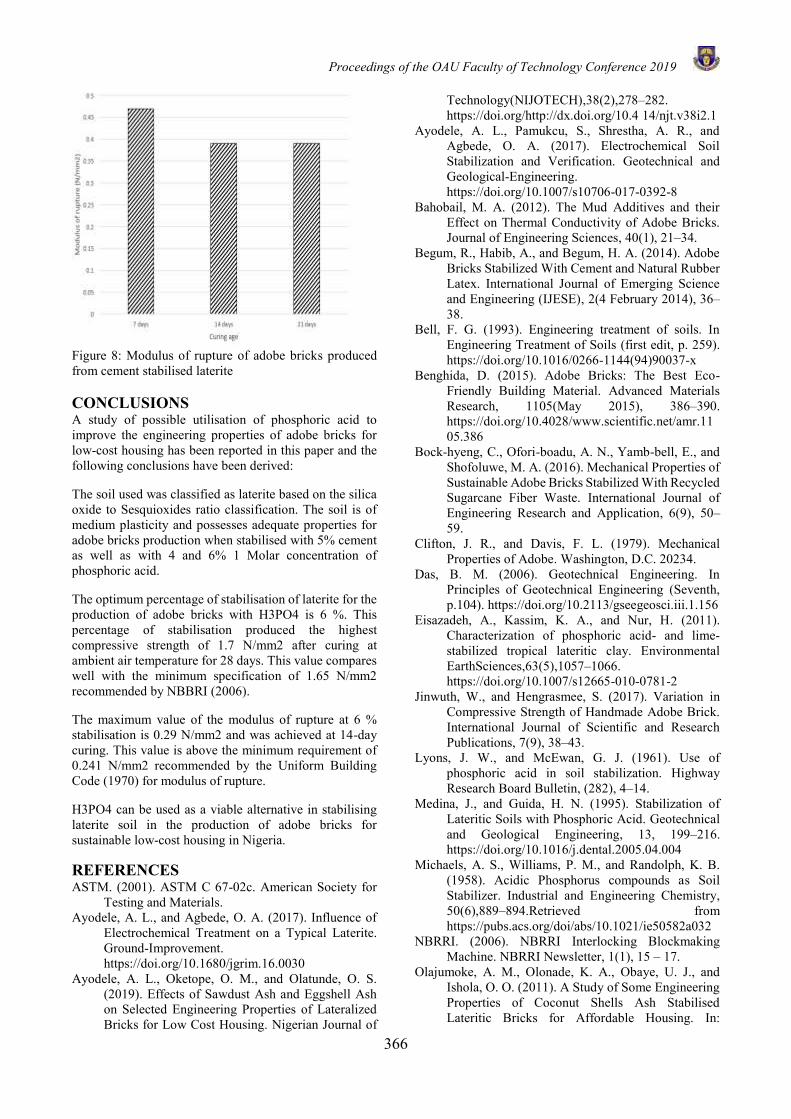
Proceedings of the OAU Faculty of Technology Conference 2019
366
Figure 8: Modulus of rupture of adobe bricks produced from cement stabilised laterite CONCLUSIONS A study of possible utilisation of phosphoric acid to improve the engineering properties of adobe bricks for low-cost housing has been reported in this paper and the following conclusions have been derived:
The soil used was classified as laterite based on the silica oxide to Sesquioxides ratio classification. The soil is of medium plasticity and possesses adequate properties for adobe bricks production when stabilised with 5% cement as well as with 4 and 6% 1 Molar concentration of phosphoric acid.
The optimum percentage of stabilisation of laterite for the production of adobe bricks with H3PO4 is 6 %. This percentage of stabilisation produced the highest compressive strength of 1.7 N/mm2 after curing at ambient air temperature for 28 days. This value compares well with the minimum specification of 1.65 N/mm2 recommended by NBBRI (2006).
The maximum value of the modulus of rupture at 6 % stabilisation is 0.29 N/mm2 and was achieved at 14-day curing. This value is above the minimum requirement of 0.241 N/mm2 recommended by the Uniform Building Code (1970) for modulus of rupture.
H3PO4 can be used as a viable alternative in stabilising laterite soil in the production of adobe bricks for sustainable low-cost housing in Nigeria.
REFERENCES ASTM. (2001). ASTM C 67-02c. American Society for
Testing and Materials. Ayodele, A. L., and Agbede, O. A. (2017). Influence of
Electrochemical Treatment on a Typical Laterite. Ground-Improvement. https://doi.org/10.1680/jgrim.16.0030
Ayodele, A. L., Oketope, O. M., and Olatunde, O. S. (2019). Effects of Sawdust Ash and Eggshell Ash on Selected Engineering Properties of Lateralized Bricks for Low Cost Housing. Nigerian Journal of
Technology(NIJOTECH),38(2),278–282. https://doi.org/http://dx.doi.org/10.4 14/njt.v38i2.1
Ayodele, A. L., Pamukcu, S., Shrestha, A. R., and Agbede, O. A. (2017). Electrochemical Soil Stabilization and Verification. Geotechnical and Geological-Engineering. https://doi.org/10.1007/s10706-017-0392-8
Bahobail, M. A. (2012). The Mud Additives and their Effect on Thermal Conductivity of Adobe Bricks. Journal of Engineering Sciences, 40(1), 21–34.
Begum, R., Habib, A., and Begum, H. A. (2014). Adobe Bricks Stabilized With Cement and Natural Rubber Latex. International Journal of Emerging Science and Engineering (IJESE), 2(4 February 2014), 36–38.
Bell, F. G. (1993). Engineering treatment of soils. In Engineering Treatment of Soils (first edit, p. 259). https://doi.org/10.1016/0266-1144(94)90037-x
Benghida, D. (2015). Adobe Bricks: The Best Eco-Friendly Building Material. Advanced Materials Research, 1105(May 2015), 386–390. https://doi.org/10.4028/www.scientific.net/amr.1105.386
Bock-hyeng, C., Ofori-boadu, A. N., Yamb-bell, E., and Shofoluwe, M. A. (2016). Mechanical Properties of Sustainable Adobe Bricks Stabilized With Recycled Sugarcane Fiber Waste. International Journal of Engineering Research and Application, 6(9), 50–59.
Clifton, J. R., and Davis, F. L. (1979). Mechanical Properties of Adobe. Washington, D.C. 20234.
Das, B. M. (2006). Geotechnical Engineering. In Principles of Geotechnical Engineering (Seventh, p.104). https://doi.org/10.2113/gseegeosci.iii.1.156
Eisazadeh, A., Kassim, K. A., and Nur, H. (2011). Characterization of phosphoric acid- and lime-stabilized tropical lateritic clay. Environmental EarthSciences,63(5),1057–1066. https://doi.org/10.1007/s12665-010-0781-2
Jinwuth, W., and Hengrasmee, S. (2017). Variation in Compressive Strength of Handmade Adobe Brick. International Journal of Scientific and Research Publications, 7(9), 38–43.
Lyons, J. W., and McEwan, G. J. (1961). Use of phosphoric acid in soil stabilization. Highway Research Board Bulletin, (282), 4–14.
Medina, J., and Guida, H. N. (1995). Stabilization of Lateritic Soils with Phosphoric Acid. Geotechnical and Geological Engineering, 13, 199–216. https://doi.org/10.1016/j.dental.2005.04.004
Michaels, A. S., Williams, P. M., and Randolph, K. B. (1958). Acidic Phosphorus compounds as Soil Stabilizer. Industrial and Engineering Chemistry, 50(6),889–894.Retrieved from https://pubs.acs.org/doi/abs/10.1021/ie50582a032
NBRRI. (2006). NBRRI Interlocking Blockmaking Machine. NBRRI Newsletter, 1(1), 15 – 17.
Olajumoke, A. M., Olonade, K. A., Obaye, U. J., and Ishola, O. O. (2011). A Study of Some Engineering Properties of Coconut Shells Ash Stabilised Lateritic Bricks for Affordable Housing. In:

Proceedings of the OAU Faculty of Technology Conference 2019
367
Proceeding of the Faculty of Technology Conference on: Innovative Technoogies for Socio-Economic Transformation in Developing Countries. Ile-Ife, Nigeria, 89–95.
Sahu, M. K., and Singh, L. (2017). Critical Review on Types of Bricks Type 4: Adobe Bricks. International Journal of Mechanical And Production Engineering., (11), 116–119.
Salim, R. W., Ndambuki, J. M., and Adedokun, D. A. (2014). Improving the bearing strength of sandy loam soil compressed earth block bricks using Sugercane Bagasse Ash. Sustainability (Switzerland), 6(6), 3686–3696. https://doi.org/10.3390/su6063686
Sharma, V., Vinayak, H. K., and Marwaha, B. M. (2015). Enhancing sustainability of rural adobe houses of hills by addition of vernacular fiber reinforcement. International Journal of Sustainable Built Environment, 4(2), 1–11. https://doi.org/10.1016/j.ijsbe.2015.07.002
Smith, E. W., and Austin, G. S. (1989). Adobe, Pressed-Earth, and Rammed-Earth Industries in New Mexico. New Mexico: Authority of State of New Mexico, NMSA.
Sriwattanaprayoon, N. (2014). Engineering Properties of Adobe Brick for Earth Structures. International Journal of Environmental and Rural Development, 5(2), 41–46.
Terzaghi, K., Peck, R. B., and Mesri, G. (1996). Physical properties of soils. Soil Mechanics in Engineering Practice (Third edit). John Wiley & Sons, Inc. New York.
Uniform Building Code. (1970). International Council of Building Officials.
Wahabi, M. A. (2017). Effects of Natural Rubber Latex in Stabilizing Adobe Bricks. Unpublished M.Sc Thesis, 55–60.
Proceedings of the OAU Faculty of Technology Conference 2019
368
DEVELOPMENT OF SUGENO FUZZY CONTROLLED TRAFFIC SYSTEM FOR Y-ROAD INTERSECTION – UNIVERSITY OF IBADAN CASE STUDY
O.E. Adetoyi Department of Electrical and Electronic, University of Ibadan, Ibadan, Nigeria.
ABSTRACT Traffic congestion is a common phenomenon in urban centres, due to large population of vehicles and limited road networks. This is especially true of developing countries where such roads are often in poor state of disrepair. A good traffic management system is necessary to make such roads safer and economically more efficient. Solutions that are based on fixed timing have the disadvantage of being unable to dynamically change with respect to the varying traffic density and presence of emergency vehicle. This paper presents a smart traffic control system capable of detecting traffic density and presence of emergency vehicle with its priority level in real time. A fuzzy inference system was designed, which takes in traffic density and ambulance priority level as input variables. The decision of which road or lane is assigned the green light and for what duration was determined by the fuzzy rules. The surface’ plot of the input variables against the output variable showed that the green phase duration varied dynamically with traffic conditions. The fuzzy controller is an intelligent approach to traffic management. Keywords: Traffic Congestion, Fuzzy Controller, Fuzzy Inference System, Intelligent Traffic Control, Smart Traffic System and Emergency Priority Level INTRODUCTION Traffic congestion is a major problem of many urban centres all over the world. This often creates adverse effect on the economy, developmental goals, cost of living, life span and general well-being of the people (Liu, Chen and Xue, 2017) (Avatefipour and Sadry, 2018). The factors responsible for traffic congestion can be attributed to large vehicular movement, inadequate road networks, bad condition of roads and absence or poor traffic signals management scheme (Lah et al., 2017). The main goals of traffic signals management scheme are to ensure traffic safety at the intersections, maximized intersections’ capacity and minimized vehicles delays. The conventional static method of traffic signal management allocates fixed green-light duration to each road or lane irrespective of the traffic condition; such as accidents, road-works or breakdown vehicles (Ghazal et al., 2016). This often results in unacceptable delays (Gacovski, Deskovski and Veljanovska, 2012) (Ghazal et al., 2016). Improvement to fixed time controller can be found in (Ghazal et al., 2016) (Faheem, Zainudin and Ahmad-Kayani, 2017). These methods are still unable to meet up with traffic dynamics like the static method, and the responsiveness is slow. Dynamic or intelligent green-phase time allocation often depends on traffic density estimate through processing of wireless sensor signals or camera images (Lah et al., 2017) (Faria et al., 2017). Among the applicable sensors type are: infra-red, combination of infra-red and magnetic, magnetometer, and photo-electric. It is essential that any method adopted is able to accurately detect vehicles to prevent false or missed detection. A more encompassing
intelligent traffic system can factor in the presence of emergency vehicles, flooding, barricade, and accident occurrence capabilities (Faria et al., 2017) (Scalabrin et al., 2017) (Satwik et al., 2018). The data required for decision making are often collected via sensors, or camera images, and these are transferred from vehicle to vehicle, vehicle to infrastructure, or infrastructure to infrastructure, by the Vehicular Ad-hoc Network (VANET), Bluetooth, Wi-Fi or Internet of Things (IoT) (Faria et al., 2017). This process of traffic data acquisition is referred to as vehicular monitoring, and it is the backbone of good traffic management system (Scalabrin et al., 2017) (Lah et al., 2017). The complexity of the decision making algorithm is usually a function of traffic parameters and acceptable level of service. One approach of managing the decision making process is through fuzzy inference system (FIS). The FIS was utilised in (Jin, Ma and Kosonen, 2017) to determine the extension time of the current green phase based on the assigned weights of all the red phase and the gap between two approaching vehicles from the intersection. The FIS was also employed in (Zade and Dandekar, 2012) to estimate green phase extension time based on traffic density and traffic flow rate data. In this paper, the FIS approach was used to determine which lane gets the green phase and for what duration based on the traffic density and the presence and priority level of ambulance. MATERIALS AND METHODS Road Intersection Model The intersection A of Figure 1 shall be considered for this design. It consists of two approaches, three movements and a traffic-light controller. Traffic flow from Ojoo end can go through the intersection to Sango or turn into
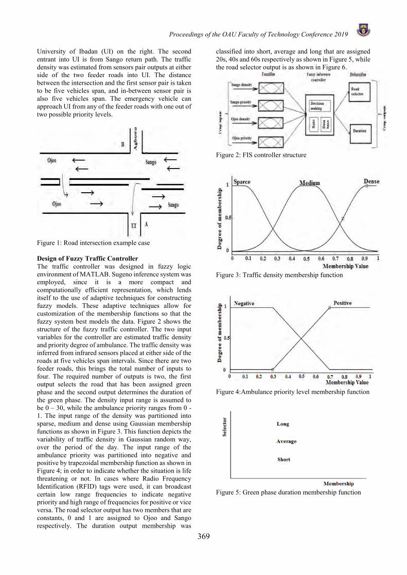
Proceedings of the OAU Faculty of Technology Conference 2019
369
University of Ibadan (UI) on the right. The second entrant into UI is from Sango return path. The traffic density was estimated from sensors pair outputs at either side of the two feeder roads into UI. The distance between the intersection and the first sensor pair is taken to be five vehicles span, and in-between sensor pair is also five vehicles span. The emergency vehicle can approach UI from any of the feeder roads with one out of two possible priority levels.
Figure 1: Road intersection example case Design of Fuzzy Traffic Controller The traffic controller was designed in fuzzy logic environment of MATLAB. Sugeno inference system was employed, since it is a more compact and computationally efficient representation, which lends itself to the use of adaptive techniques for constructing fuzzy models. These adaptive techniques allow for customization of the membership functions so that the fuzzy system best models the data. Figure 2 shows the structure of the fuzzy traffic controller. The two input variables for the controller are estimated traffic density and priority degree of ambulance. The traffic density was inferred from infrared sensors placed at either side of the roads at five vehicles span intervals. Since there are two feeder roads, this brings the total number of inputs to four. The required number of outputs is two, the first output selects the road that has been assigned green phase and the second output determines the duration of the green phase. The density input range is assumed to be 0 – 30, while the ambulance priority ranges from 0 -1. The input range of the density was partitioned into sparse, medium and dense using Gaussian membership functions as shown in Figure 3. This function depicts the variability of traffic density in Gaussian random way, over the period of the day. The input range of the ambulance priority was partitioned into negative and positive by trapezoidal membership function as shown in Figure 4; in order to indicate whether the situation is life threatening or not. In cases where Radio Frequency Identification (RFID) tags were used, it can broadcast certain low range frequencies to indicate negative priority and high range of frequencies for positive or vice versa. The road selector output has two members that are constants, 0 and 1 are assigned to Ojoo and Sango respectively. The duration output membership was
classified into short, average and long that are assigned 20s, 40s and 60s respectively as shown in Figure 5, while the road selector output is as shown in Figure 6.
Figure 2: FIS controller structure
Figure 3: Traffic density membership function
Figure 4:Ambulance priority level membership function
Figure 5: Green phase duration membership function
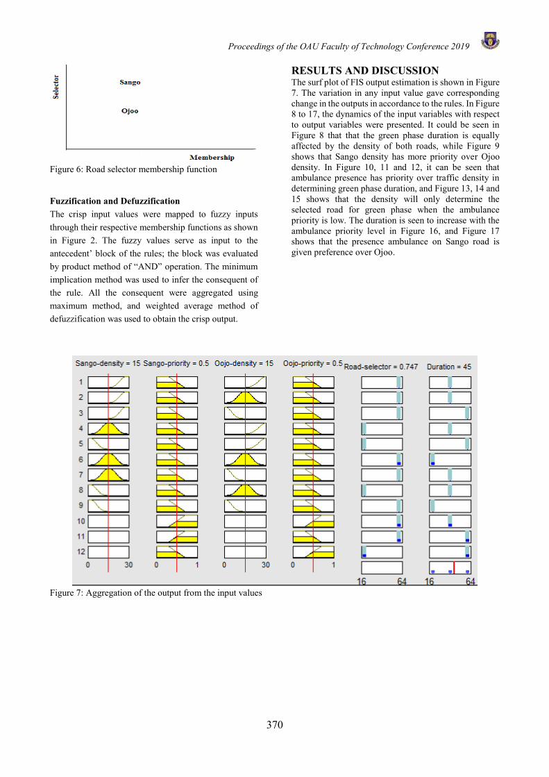
Proceedings of the OAU Faculty of Technology Conference 2019
370
Figure 6: Road selector membership function Fuzzification and Defuzzification The crisp input values were mapped to fuzzy inputs through their respective membership functions as shown in Figure 2. The fuzzy values serve as input to the antecedent’ block of the rules; the block was evaluated by product method of “AND” operation. The minimum implication method was used to infer the consequent of the rule. All the consequent were aggregated using maximum method, and weighted average method of defuzzification was used to obtain the crisp output.
RESULTS AND DISCUSSION The surf plot of FIS output estimation is shown in Figure 7. The variation in any input value gave corresponding change in the outputs in accordance to the rules. In Figure 8 to 17, the dynamics of the input variables with respect to output variables were presented. It could be seen in Figure 8 that that the green phase duration is equally affected by the density of both roads, while Figure 9 shows that Sango density has more priority over Ojoo density. In Figure 10, 11 and 12, it can be seen that ambulance presence has priority over traffic density in determining green phase duration, and Figure 13, 14 and 15 shows that the density will only determine the selected road for green phase when the ambulance priority is low. The duration is seen to increase with the ambulance priority level in Figure 16, and Figure 17 shows that the presence ambulance on Sango road is given preference over Ojoo.
Figure 7: Aggregation of the output from the input values
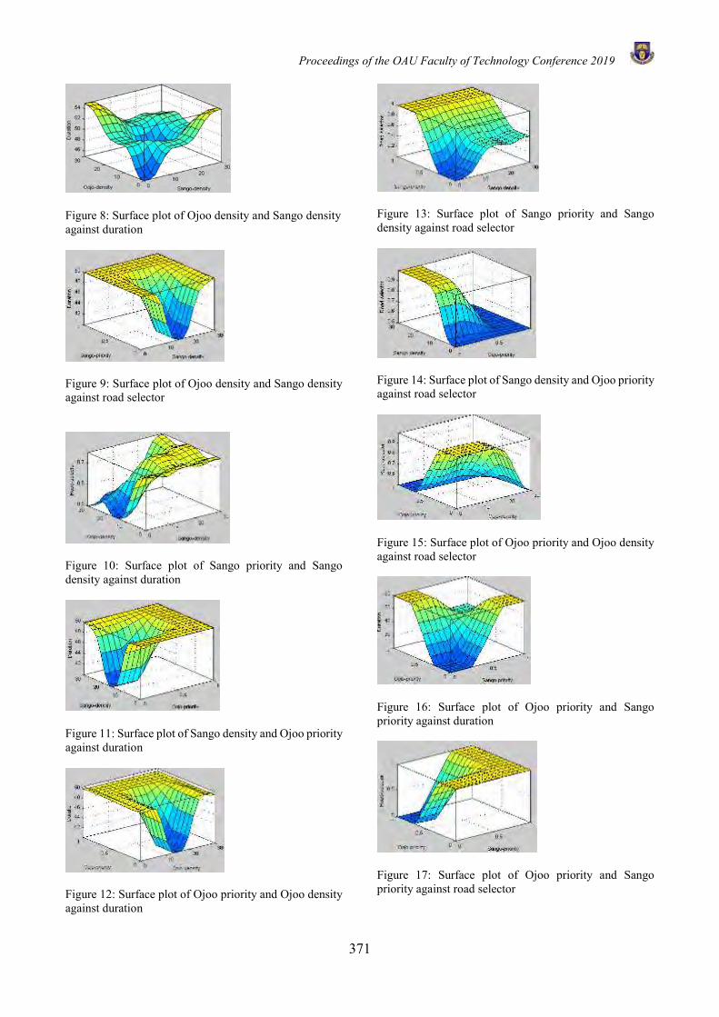
Proceedings of the OAU Faculty of Technology Conference 2019
371
Figure 8: Surface plot of Ojoo density and Sango density against duration
Figure 9: Surface plot of Ojoo density and Sango density against road selector
Figure 10: Surface plot of Sango priority and Sango density against duration
Figure 11: Surface plot of Sango density and Ojoo priority against duration
Figure 12: Surface plot of Ojoo priority and Ojoo density against duration
Figure 13: Surface plot of Sango priority and Sango density against road selector
Figure 14: Surface plot of Sango density and Ojoo priority against road selector
Figure 15: Surface plot of Ojoo priority and Ojoo density against road selector
Figure 16: Surface plot of Ojoo priority and Sango priority against duration
Figure 17: Surface plot of Ojoo priority and Sango priority against road selector
Proceedings of the OAU Faculty of Technology Conference 2019
372
CONCLUSION The FIS approach of allocating green phase timer, while taking ambulance presence and priority into cognisance offers effective and efficient means of traffic management. It offers superior performance over improved fixed timer or FIS green phase extension, since it can dynamically respond to traffic conditions. REFERENCES Avatefipour, O. and Sadry, F. (2018) 'Traffic
Management System Using IoT Technology - A Comparative Review', IEEE International Conference on Electro/Information Technology (EIT), Michigan, 1-6.
Faheem, F., Zainudin, Z. and Ahmad-Kayani, A. (2017) 'Optimization of Vehicle Actuation and Multiplan Algorithms for Urban Traffic Control Systems', IEEE Conference on Systems, Process and Control (ICSPC), Melaka, Malaysia, 59-64.
Faria, R., Brito, L., Baras, K. and Silva, J. (2017) 'Smart Mobility: A Survey', International Conference on Internet of Things for the Global Community (IoTGC), Funchal, Portugal.
Gacovski, Z., Deskovski, S. and Veljanovska, K. (2012) 'Fuzzy Traffic Controller for Urban Intersection Developed in Simulink/SimEvents', 13th IFAC Symposium on Control in Transportation Systems, Sofia, Bulgaria, 122-125.
Ghazal, B., EIKhatib, K., Chahine, K. and Kherfan, M. (2016) 'Smart Traffic Light Control System', Third International Conference on Electrical, Electronics, Computer Engineering and their Applications (EECEA), Beirut, Lebanon, 140-145.
Jin, J., Ma, X. and Kosonen, I. (2017) 'An intelligent control system for traffic lights with simulation-based evaluation', Control Engineering Practice, vol. 58, pp. 24-33.
Lah, A.A.A., Latiff, L.A., Dziyauddin, R.A., Kaidi, H.M. and Ahmad, N. (2017) 'Smart Traffic Monitoring and Control Architecture and Design', IEEE 15th Student Conference on Research and Development (SCOReD), Putrajaya, Malaysia, 72-76.
Liu, S.V., Chen, F. and Xue, J. (2017) 'Evaluation of Traffic Density Parameters as an Indicator of Vehicle Emission-Related Near-Road Air Pollution: A Case Study with NEXUS Measurement Data on Black Carbon', International Journal of Environmental Research and Public Health, vol. 14, no. 12.
Satwik, C.V.A., Kumar, L.P., Vineeth, K. and NPillai, K. (2018) 'Intelligent Road Management System for Daily Transit', International Conference on Communication and Signal Processing, Chennai, India, 523-526.
Scalabrin, M., Gadaleta, M., Bonetto, R. and Rossi, M. (2017) 'A Bayesian Forecasting and Anomaly Detection Framework for Vehicular Monitoring Networks', International Workshop on Machine Learning for Signal Processing, Tokyo, Japan.
Zade, A.R. and Dandekar, D.R. (2012) 'Simulation of Adaptive Traffic Signal Controller in MATLAB
Simulink Based On Fuzzy Inference System', National Conference on Innovative Paradigms in Engineering & Technology (NCIPE), Nagpur, India, 9-13.

RE-THINKING ENGINEERING EDUCATION FOR SUSTAINABLE
HUMAN DEVELOPMENT
O. A. O. DE. JO. BIComputer Science and Engineering DepartmentO. bafe.mi Awolo.wo. University, Ile-Ife. , [email protected] ; [email protected]
ABSTRACT
The research literature on the subject matter of engineering education is rich in diverse principles, philosophies andtheories. These have manifested in the formulation of policies that have been used to create and operate severalteaching and learning models. However, an analysis of the findings, as documented in the discourse presented in theliterature, suggests that a consensus is yet to emerge on the most effective and sustainable model that must be adoptedin the training of engineers, particularly in African countries. There is a divergence of, and sometimes contradictory,opinion on how engineers should be educated for the purpose of sustainable human development in Africa. This issue isparticularly worrisome in the context of the realisation that a sound education model is necessary, though not sufficient,for a successful engineering career.
This paper interrogates the principle, philosophy and theories of education as institutionalised in the indigenousculture of the Yoruba people. An epistemological analysis of narratives in the discourse about and around Yorubainstitutions and league of professionals such as the Alagbe. de. (Metalworkers), O. de. (Hunters), Alaro (Dye workers),Ahuns.o. (Cloth Weaves) and so on, was conducted. The results were then interpreted based on the criteria of respon-sive, purposeful and sustainable educational model. The findings suggest that it is safe to conclude that the educationalprinciples and philosophy underpinning indigenous Yoruba professions, have great potential for adaptation and adoptionas conceptualisation instrument in the formulation of a teaching and learning model for Nigerian engineering education.keywords: Education, Engineering, Africa, Yoruba culture.
1 INTRODUCTION
The intention here is to invite intellectuals, educators andacademics to a serious dialogue on issues relating to afundamental question for engineering education in mod-ern Nigeria. That question is: “what really does it meanto educate competent engineers for successful performancein Nigerian, and perhaps African, society?” The need toarticulate a succinct narrative that answers this questionemerges in the context of contemporary experiences of com-plaints, with overwhelming evidences, of the poor perfor-mances of engineering graduates of Nigerian tertiary insti-tutions. A synthesis of these complaints seems to suggestthat engineering education in Nigerian tertiary institutionsis not preparing graduates for creditable and competentprofessional life. Graduates seem unable to consciously ap-prehend the awareness of their immediate environment, atleast well enough, to be able to design and operationalisetechnologies that responds effectively to societal needs. En-gineering education seems, therefore, to have taught gradu-ates to be mentally and materially “dead” to their own cul-tural and natural environmental needs. The present situa-
tion therefore makes it expedient for teachers, researchersand students to reflect on the substance of the fundamentalprinciples underlying Nigerian engineering education. Theintention here is not to provide a definitive answer to thequestion raised in this paper, though. Nonetheless a robustargument to engender conference debate on the appropri-ate formulation of the core concepts for effective engineer-ing education will be advanced. This is with the view tospurring a fruitful intellectual engagements that will fur-ther crystallise our understanding of the subject matter.In Section 2 the etymology of important lexical items inengineering vocabulary were re-examined. Section 3 is adiscussion on selected core issues in engineering educationfrom an indigenous African perspective. Section 4 pre-sented selected cases of education models used in Yorubasettings. The summary and conclusion of this conferencepaper are presented in Sections 5 and 6, respectively.
2 WHAT IS ENGINEERING
Who is an engineer and what constitutes the substance ofthe processes by which the person assumes that status?
373
Proceedings of the OAU Faculty of Technology Conference 2019
Before we start to address the issue of engineering edu-cation it is important to provide an explanation for ourconception of the term “engineer” (Chambers, 1985; Stod-dart, 1999). The word “engine”, which is the root word forengineer, originates from Greek and it means “any devicethat converts energy to power”.
The etymology (study of the root, origin and devel-opment of words) of the term engineer situates it in theEuropean epistemology. According to the Online Etymol-ogy Dictionary (EtyDico, 2019), the noun form of the termengineer is an ancient Greek word mekhanopoios: whichmean a “maker of engine”. The concept entered into Latinfrom Greek as ingeniare. In medieval Latin, the term wasuse in the civil sense to mean “public works” (Halsey,1899). The Latin form enter into Old French as engig-neor which means “constructor of military engines”. Theconcept took a new form enginour in modern French tomean “inventor, designer” which also implies “engineer,architect, maker of war-engines; schemer”. The term “en-gineer” entered into the British English from French andwas first used in American English in about 1830, to mean“locomotive driver” (EtyDico, 2019).
As a verb, the term engineer is the process used by en-gineers (the noun) to “arrange, contrive, guide or manage(via ingenuity or tact)”. The word “engineered”, in mid-dle English has a verb “engine” that means “contrive, con-struct”. It is also used to mean “seduce, trick, deceive, aswell as ‘put to torture’ ”(EtyDico, 2019). The Online Ox-ford Dictionary (OxfDico, 2019) defines engineer as a per-son who designs, builds, or maintains engines, machines,or public works. Its synonyms include designer, planner,builder, architect, producer, fabricator, developer, creator,inventor, originator, deviser, contriver, mastermind.
Based on the above etymological analysis, it is clearthat the contemporary view, conception and semantics ofthe term “engineer”, either as a noun or a verb, is stronginfluenced by the European perspectives. What is clearfrom the various conceptions of the term “engineer” is thatit involves the knowledge and capability to make devicesthat converts energy into power. The power can then beused to form and transform materials in order to addresshuman needs. This conception situates engineering in thenexus between knowledge and human needs. To this end,the substance of engineering education should be situatedwithin the domain of knowledge and human needs. Sinceknowledge is acquired through education, whenever soci-etal needs are not satisfied due to ineffective deploymentof knowledge, the place to start a purposeful interrogationis the fundamental principles underpinning the educationsystem.
3 ISSUES IN ENGINEERINGEDUCATION
Education takes place in an environment comprising two(2)active agents, namely: (i) The Teaching Agent(TA) and(ii) the Learning Agent (LA). The TA and LA must en-
gage in a purposeful interaction over a period of time. Thepurpose of the interaction is to exchange knowledge andsharpen understanding, individually and collectively, abouta subject matter of mutual interest. An effective purposefor education is constructed based on a conscious appraisalof the past in the context of current needs with an eye onfuture projections. For education to be purposeful there-fore, it must be rooted in the experiences of the past (em-bodied in the teachers, TA), respond to the need of thepresent (manifesting in current societal needs) and projectan enduring hope for the future (embodied in the students,LA). For a purposeful engineering education to respond tothe needs of an environment, it must be situated withinconscious awareness of the everyday experiences of the TAand LA in that environment.
The interaction between the TA and LA in an educa-tional environment should engender the creation of knowl-edge in a continuum in which the status-quo is continu-ously interrogated and refined through purposeful mentalengagements. Such interaction, must posit knowledge asthe fundamental currency of engagement. The desire tocreate knowledge, acquire knowledge, use knowledge, keepknowledge, expand and refine knowledge, prevent the adul-teration of knowledge and institutionalised the acquisitionof knowledge will then be the guiding principle. To main-tain the substance of its purpose therefore, knowledge asthe currency for exchange cannot itself, become a commod-ity of exchange.
Education is situated within a way of knowing. Theway of knowing will define and characterise what consti-tutes knowledge, the performance criterial for determiningcompetence, identity of areas of knowledge, the value asso-ciated with the acquisition and possession of knowledge aswell as the model of the institution of knowledge (Afo.nja,1986; Mazzochi, 2006). Three of the core principles thatare peculiarities to the European way of knowing are herediscussed in contrast to an African way of knowing, in thiscase, the Yoruba. These are:
1. The concept and philosophy of knowledge and itspurpose in education;
2. The Language of engineering education;
3. The institution and instrument of education.
These, in my view, are the core issues to which ade-quate answers must be proffered in the task of formulationan effective model for indigenous Nigerian, and perhapsAfrican, engineering education. They will be further dis-cussed in the sequel.
3.1 Issue 1: Concept and philosophy
As stated in Section 2, the model of engineering educa-tion in Nigeria, and perhaps many African countries, isstrongly influenced by the European perspectives and tra-ditions. Central to this model is the philosophy, or concept,of knowledge (epistemology) and its purpose in within aneducational enterprise. To situate our answer in the proper
374
3.1 Issue 1: Concept and philosophy Proceedings of the OAU Faculty of Technology Conference 2019
context, we need to address two issues: (i) What is knowl-edge and (ii) What is the purpose for its acquisition. Toknow something, as opposed to not knowing it, is a func-tion of many factors. Formally, given a natural object X,if a person p1 makes the claim that “I known X”, does thisimply the same thing when another person p2 makes thesame claim that “I known X”? These are epistemologicalissues that are outside the purview of this paper. Whatis clear, however, is that knowledge is innate, so also arethe competence to exercise its performance. There is nouniversal knowledge of a natural object X to which everyperson has the same semantic subscription. In the realm ofknowledge, the European truism of perfect identity “like-ness is sameness”(Jones, 1900) does not apply.
In the European way of knowing, which constitutes thepedagogy of modern engineering education in Nigerian, theprimary purpose of the acquisition of knowledge in educa-tion is: knowledge is power. Power, in this context, is in-terpreted to mean the capacity to conquer, dominate andcontrol. The tendency for the survival of the fittest syn-drome, engenders an unregulated competitive social ordermodelled in a manner reminiscence of a crude interpreta-tion of the Charles Darwin’s evolution theory. This hasprecipitated primitive accumulation of knowledge for thesake of power for self aggrandisement. This has resultedin a world in which, despite evidences of rapid “advance-ment in knowledge”, the criteria of performance continuesto defeat the innate human desire for sustainable peacefullife and living.
This European principle of education manifest in thedefinition of the purpose of education for European andallied nations. This is well articulated by Bayyinah Bello(Bello, 2010) and manifests in the British and Americaneducational systems as follows.
1. The purpose of education in Britain is to train BritishSubjects. A British Subject is someone who is sub-servient to the British royalty in a manner reminis-cence of the relation between servants and their lords.
2. The purpose of education in the United States ofAmerica is to train American Citizens. An Amer-ica Citizen is someone who must defend the Ameri-can constitution, and if necessary, using the force ofarms.
The wholesale application of the European philosophyof education has institutionalised a semblance of learning,producing clever graduates that know the best ways to earna living from the people; not the best way of earning properliving with the people. The consequence of this are grad-uates who see no future in their immediate environmentwith a parasitic outlook engendering a mindset of unbri-dled entitlement on the people and society (Lawal, 1987).
The Yoruba, and perhaps other African and oriental,concept of knowing is radically different from the Euro-pean model. The following are a few of the Yoruba apho-risms that explicates the substance of the Yoruba conceptof knowledge in the context of education:
(i.) O. gbo. n laa fi gun e. s. in ımo. de ıbute iyı. Translatesas: “Intelligence is what we use to ride the horse ofknowledge to the destination of dignity”.
(ii.) Mo gbo. ntan mo mo. o. tan; awo ılu awo. n omungo. .Translates as: “ ‘I understand it all’, ‘I know it all’, isthe substance of the theory of stupidity”. Arroganceis the most potent evidence of ignorance.
(iii.) Iwa dun onımo. ımo. di egun; o. gbo. n dun alagbara,agbara di aaganan. Translates as: “ Knowledge with-out character manifests in curse: power without in-telligence manifests in erraticism.”
(iv.) O. gbo. n ju agbara lo. , nıtorı alagbara ma mero nibaba o. le. . Translates as: “Intelligence is greater thatpower, powerfulness without intelligence is the pro-genitor of powerlessness.” This is in contrast to theEuropean “knowledge is power” aphorism.
(v.) Bıi were ni o. gbo. n, ijo. tı o. lo. gbo. n ba mo. pe ohun gbo. n,ni ago re. be. re. ; Translates as: “Intelligence is likemadness, stupidity starts when the intelligent per-son is aware of his intelligence”
(vi.) O. gbo. n o. dun nıı, omungo. e. e. mın; Translates as: “Thisyear’s intelligence is the foolishness of next year”
In the aphorism listed above, knowledge is conceptu-alised as an instrument that requires intelligence for itsfruitful application. The fundamental aim of education,therefore, is not the acquisition of knowledge for the pur-pose of power. The principle of education is to initiate aself-awareness that motivates the individual to recognisethe importance, extent and limit of knowledge. An edu-cation that inculcates the understanding that knowing isthe beginning of the journey towards self-realisation andfulfilment, not that for power over others. An awarenessthat engenders a strong desire to want to know and to treatthe known like a drop of water in the sea of knowable. Aself-awareness that engenders the outlook of the humilitythat makes the individual to recognises power as a conse-quence, not the purpose of knowing. An awareness whichmanifests in the understanding that power is meaningfuland purposeful only when exercised in the context of har-mony with nature. This paradigm posit knowledge in thecontext of its use for living in harmony with nature in allits tangible and intangible manifestations.
Within the Yoruba epistemology therefore, knowledgeis not Justified True Belief (JTB) (Gettier, 1966). Indeedknowledge is a tentative, and necessarily incomplete, truthsituated within the experiences of individuals. To be use-ful, therefore, the knowledge of each and every knower mustbe intertwined so tightly that the whole will work togetherin unison (Bo.dunrın, 1974; Ogunne.ye., 1984). Within thiscosmos, human experience of nature is an holistic conceptin that it is an integration of all the known taken overall the members of the community of knower. No lan-guage can integrate and formulate these experiences into awhole. Hence, human experiences expressed in language isnecessarily incomplete and hence always tentative. In the
375
3.2 Issue 2: Language of education Proceedings of the OAU Faculty of Technology Conference 2019
Yoruba cosmos, therefore, knowledge is Tentatively Con-ceived human experience of Nature (TCN).
The Oxford Advanced Learners Dictionary, defines ed-ucation as “ a process of teaching and learning, especiallyin schools or colleges, to improve knowledge and developskills”. E. ko. is the Yoruba equivalent term for education.E. ko. is the noun and verb forms of a concept whose mean-ing is morphologically encoded into a two-syllable word:(1) E. and (2) ko. . The first syllable, that is E. , qualifies thesecond one, ko. . Ko. has a compendium of meaning whichincludes: (i) teach, (ii) build and (iii) hang or place overa hook. All these connotes an important dimension in thesemantic space into which the Yoruba concept of educa-tion is projected. The meaning of education subsumes thebuilding of human character and tending it to hang prop-erly to work in harmony with societal needs and norms.There are generally two kinds of E. ko. . E. ko. Ile, “home edu-cation” and E. ko. ode “town education”. The responsibilityfor these forms of education is on the society. Alaıle. e. ko. o.is an insult targetted at a person who demonstrates defi-ciency in any of these forms of education. If the cause of thedemonstrated educational deficiency is the teacher, the in-sult Abııko. is targeted at the teachers or parents. Ako. o. gbais an insult targeted at a person who refuses educationalinstruction. Either of these insults will elicit serious re-flections, and sometimes, violent response from the personbeing insulted (Akınye.mı, 2015).
The purpose of Yoruba education is not to train sub-jects that are subservient to a royalty, as is the case inthe British model. It is also not about training individ-uals with military posture, as is the case in the Ameri-can model. Indeed the purpose of Yoruba education isto develop individuals to be come o. mo. luabı (o. mo. tı oluıwa bı) (O. de.jo. bı, 2015). A person is o. mo. luabı if the sub-stance of his or her character manifests humility (Ire. le. ),modesty( Iwo. ntuwo. nsı), self-discipline (Ikorae. ninıjanun),indomitable spirit (Ifo. kanran), honesty (Otıto. ) and perse-verance (Ifarada). The summative effect of this manifes-tation is respect (O. wo. ) for humanity and nature. Suchperson will, through the performance of his or her pro-fessional duties, pay due diligence to, and respect for, so-cial norms and processes, even when in disagreement withthem. Such persons will also be expected to be industriousand creative. This model resonates well with other Africanand, perhaps, oriental cultures (Khanna, 1994; Chang andLee,1998; Jagusah, 2001; Wang, 2006).
3.2 Issue 2: Language of education
The influence of language on the process and product ofthoughts is often underestimate, particularly in engineer-ing education. This is despite overwhelming arguments,supported with experiences and strong historical evidences,that the language of instruction is the most powerful in-strument in the toolbox of effective education (Fafunwa,1974; Rubayumya, 1999; Brock-Utne, 2001; Vukovic andLesaux, 2013). In a broad sense, language influences howthe things that come into conscious awareness are reckoned,
registered, rendered and memorised. Language also influ-ences the character, scope and extent of the insight that istaken into account during observations. Furthermore, theconception and construction of experiences in terms of howthey are formulated, translated, interpreted and narratedis a function of the linguistic tools and devices availablein the language of expression (Bamgbos.e, 1983; E. kundayo. ,1986; Chomsky, 2006; Lesaux, 2013; Borodirsky, 2011).
For example, the logic of discourse in a language willdetermine whether or not a statement is accepted as cor-rect or incorrect (O. de.jo. bı, 2017). The nuance of a languagewill also affect the encoding, decoding and interpretationof facts. For example, culture specific metalinguistic signa-tures, such as eye-contact, tone or stress patterns, accom-panying the articulation of a statement will determine thecharacter of its information contents. The prosody accom-panying a statement may influence the seriousness withwhich the fact or evidence being expressed is to be takeninto account. Fundamentally, therefore, the creative forcefacilitated by the instrument of language is an essential in-gredient in the engineering of things that are expected tooperate in unison with a people’s experience. It is also im-portant to note that the spoken language, which constitutethe core medium through which the substance of engineer-ing knowledge is situated, operates differently from writtenlanguage, which constitutes the core medium in which for-mal engineering communications is conducted. For a fact,not all spoken utterances can be reduced into writing.
The Yoruba word for language is ede. This is ex-panded within the Yoruba epistemology to: “ohun tı a finde ero”. Meaning, “the instrument for moulding, form-ing or formulating thoughts”. Within the Yoruba cosmos,human thought is an innate mental experience that is notamenable to complete formulation in language. By thisposition, every statement expressed in human language isnecessarily incomplete. The Karl Popper’s (Popper, 1963)falsifiability theory finds a more powerful articulation inthe Yoruba concept of the role of language in the expres-sion of knowledge. The aphorism: “ko sı ohun to nı ojutı ko nı odı” exemplifies this concept. This aphorism isinterpreted to mean: “Every concept is complementary”.Hence, anything expressed in human language is falsifiable.The implication of this, for the language of instruction, isthat there may be a universal system of language for theconstruction and expressions of shared thoughts about aconcept. However, there is no universal knowledge of aunique concept to which every human instantiates and sub-scribe. This is further explicated in the aphorism: “Irırıni ıpınle. ımo. ; ohun tı arırı kıı se e. gbe. ohun tı a gbo. rı.”,meaning:“Experience is the foundation of knowledge. Thethings that we have experienced is superior to those wehave heard”
The implication of this for engineering education is thatthe forms and contents of engineering concepts is a func-tion of what the instrument of its language can be usedto formulate and communicate. The mastery of the lan-guage used to formulate and communicate the experiencewill determine how precisely and correctly the details were
376
3.3 Issue 3: Institution and instruments Proceedings of the OAU Faculty of Technology Conference 2019
reckoned as well as its appropriateness to purpose. It isonly through the use of indigenous language that individ-ual agents (TA and LA) will be able to tap into the intan-gible intellectual resource of the society. Therefore, it isonly through an indigenous language that the engineer caninstantiate and create objects and artefacts that respondseffectively to the needs of the society. The cultural and en-vironmental context of human experiences have, perhaps,the strongest influence on its engineering needs. When apiece of engineering work is robbed of its cultural context,through the substitution or replacement by those from aforeign culture, the best that can be achieved is conformitywith partial requirements. A partial requirement cannotsatisfy a need because it will fail to adequately capture thelevel of knowledge to account for the substance of the con-cept in the world-view underlying the cultural experiences.A language that does not have the power to instantiateand construct an experience cannot make the experienceto manifest in thought. This is indeed the reason why, inthe recorded human history, no nation has emancipatedherself or developed solutions suited to her own needs byusing a foreign language.
3.3 Issue 3: Institution and instruments
Now, to the engineering education institution and instru-ments. Based on the above analysis, I will classify mod-els of educational institutions into two groups, namely: (i)Methodological and (ii) Systemic. The methodological edu-cational model has distinct input and output characterisedby well-define methods, criterial and features guiding agentengagements. The input is characterised by a set of require-ments that an agent must satisfy for admission, while theoutput is characterised by a set of criterial that an agentmust satisfy before graduation. The focus of education inthis context is to transform the learning agent, through aset of lessons on topics from a well structured syllabus ofactivities, into a graduate agent with the potential to per-form the learned task at a predetermined level of compe-tence. Graduation criteria may include the potential of theLA to becomes a TA as a result of partaking in the learn-ing activities. The methodological model of education isnecessarily analytical, reductionist and prescriptive. It isanalytical and reductionist because learning is divided intosequence of discrete tasks which are connected and mustbe presented in a predetermined order (Mazzochi, 2006;Yadav and Korb, 2012). Each task comprises carefully se-lected topics which are built into a syllabus that prescribesthe things that must be studies and mastered before ad-vancing to the next stage. Each stage is not necessarilytied to a length of exposure. It is tired to the ability todemonstrate performance through personal achievementsin prescribed set of assessments and appraisals. A placeof learning is set aside, often in the learning environment,and there is a formal procedure of interaction. The knowl-edge needs are determine a-prior and the teaching pro-cesses are structured to transmit these to the LA by the TAthrough the instrumentality of a well-defined curriculum.
The professional life of an agent is marked by a uniquepoint of entry (appointment) and a unique point of exit(retirement). This makes the methodological model linearand relatively regular, with an evaluation mechanism forguiding progress. Evaluation is for the purpose of placingindividuals on a scale of preference based on a set of pre-defined quantitative performance measures. This is withthe aim to recognise and distinguish individuals that haveperformed better than other members of their own group.
The systemic educational model is organic. Themetaphor for knowledge generation, transmission and re-generation, is community of living organisms. Agents inthe education model are viewed as organs, or parts of thewhole system, each with unique functions. The interac-tions between organs manifest in activities that culminatesin the pattern of behaviour exhibited by the entire sys-tem. The organs therefore work together in unison. Thesystem grows as a whole and the development of a part,or the improvement in its function, will necessarily roboff on those of the other parts of the system. Individu-als will be identified as LA and TA but their status willbe in the context of the role they are playing at an in-stance in the life of the system. The status evolves andchanges dynamically. Engagement in the systemic modelof education is life-long and there is no situation in whicha learner stops learning or when a teacher stops teaching.Indeed the learning and teaching tasks are in a symbioticrelationship through which the one sharpens and refinesthe other. Engagement is also not situational as the en-tire location in the learning environment becomes a placefor learning and teaching. There is no formal procedureof interaction as the teaching and learning agents respondsin unison to the knowledge required to satisfy emergingneeds of the environment. The topics, syllabus and cur-riculum are ingredients for guided and purposeful feedbackneeded to connect past, present and future activities intoa whole. Their role is to ensure that the education institu-tion maintains and sustains its identity while respondingto social and environmental needs. The birth of an indi-vidual marks entry into the system and their death markstheir exit. The concept of appointment and retirement,therefore, does not apply. The identity of the individualis built into and situated within the educational environ-ment. The role of individuals changes in line with theirstatus due to experience as a result of age or other con-sequence of nature. Hence, the systemic education modelis cyclic, context sensitive and non-linear. The evaluationinstruments is a multi-dimensional probe. Evaluation isfor the purpose of assessing the competence of individualagents in order to be able to determine how best to improvethe behavioural pattern of the entire system. This is doneby determining the best possible adjustments required tomake the parts of the system to function better together inharmony towards the sustenance of past achievements andthe realisation of common goals.
The next Section documents a re-appraisal of selectedYoruba professional guilds in order to showcase the sys-temic educational model underpinning them.
377
Proceedings of the OAU Faculty of Technology Conference 2019
4 CASES IN YORUBA EXPERI-ENCES
It will be naıve to suggest that the knowledge and skills tomake devices for converting energy to power, and indeedthe intellectualism to satisfy human material and mentalneeds, are alien to Africa. For if we take the position thatengineering and intellectual education are alien to Africa,it will be difficult for us to explain how the Nubian andEgyptian achieved the building of their pyramids and howMali came about the University of Timbuktu (Okoye, 1964;Diop, 1974). It will also be difficult to explain how theYorubas are able to create a formidable social and intel-lectual system that allowed them to smelt iron to makedifferent tools that were used in farming, hunting, buildingand cloth making as well as in the processing of a variety offood and alcohol (Zalavsky, 1970; Verran, 2001). The fab-rication of the iconic Ife. Bronze Heads could not have beenpossible in the absent of an organised system of knowing.
The engineering education in modern African statesemerged in the 19th century as a part of other Europeanthree prong “civilisation” projects formulated around reli-gious proselytizing, commerce and imperial presence on thecontinent. Before then, there are organised professionalguilds in Yoruba traditional. These include: Alagbe. de.(Blacksmith), O. de. (Hunter), Afingba (Calabash artist),Amo. koko (Porter), Alaro (Dye maker), Ahuns.o. (Weavers),O. lo. se. (Soap maker), among a host of others (Sieber, 1973;Abejide, 2001). Here we attempt a brief but faithful de-scription of three(3) of the selected guild of professionals.Though most of these skills will be classified as craft spe-cialisations in modern engineering, the import of this ap-praisal is to examine the educational model responsiblefor their survival and sustenance despite neglect since theemergence of the European modernisation enterprise.
4.1 Alagbe.de.
This is the blacksmith guild. Their profession is builtaround the smelting and fabrication of metal tools. Thetools are fabricated using mental extracted from e. ta irin,iron ore. It is a family based profession passed from fatherto son. Those born into the profession (Aje. bı) have uniqueappellate, such as ogun or owu, in their names. A non-family member wishing to practice the profession must beproposed and recommended by the head of his own family(Olorı e. bı). Such a person is adopted into the profession ina manner reminiscence to the birth of a new child with anew name given. However, the old name will normally beretained and used when appropriate. The Alagbe. de. ’s tool-box includes the following locally made implements: hardstone (o. lo. ), iron anvils (owu), iron hammers (oolu), tongs(e. mun), awl(ılu), bellows (e. wırı) and tuyere, among oth-ers. Consumables of the profession include charcoal (eedu)and palm-kernel shell (eesan). Alagbe. de. make tools such asadzes (ganbu), axes (aake), hoes (o. ko. ), hunting guns (ıbo. no. de. ), cutlasses (ada), knives (o. be. ) and swords (ida), amongothers. They also make religious relics (e.g. e. dan ogboni)
and medical implements (e.g. e. wo. n abıku) according tospecifications. In modern times they also produce crudeforms of vehicle and machinery parts. Some alagbe. de. workin conjunction with welders to produce medical, home, andsecurity equipment, for example car pedal-lucks. The craftis practised tax-free and members of the profession havecomplete immunity in their place of work. This meansthat, by tradition, it is an abomination to attack, arrest,molest or otherwise mistreat alagbe. de. , even by the king,while they are at agbe. de. , their place of work.
4.2 O. de.
This is the hunters’ guild. It is a family based professionpassed from father to son. In exceptional cases daughtersare also commissioned as O. de. , but their hunting activi-ties are closer to home (Igbe. etıle). Those born into theprofession (Aje. bı) have unique appellate, such as Ogun orO. de. , appended to their names. They can also have nick-names with “ıbo. n” as a morphemic content, for exampleAkerenbo. n, Ate. re. nbo. n, E. dunhao. n, and so on. A non-familymember wishing to practice the profession must be pro-posed and recommended by the head of his own family(Olorı e. bı). Such persons are adopted into the professionin a manner reminiscence to the birth of a child. Such per-sons will normally retain their names. Sometime however,the name O. de. wumı will be adopted.
The primary toolbox of O. de. include guns (ıbo. n) forhunting game animals, knives (o. be. ), cutlass (ada), sword(ida) and sheath (ako. ), hunting bag (apo o. de. ), amulet bag(apo o. de. ), amongst others. These tools are made by thealagbe. de. and ons. e o. na (art craftsmen) in the locality. Thehunting cloth comprises a small jacket (gberı), knee lengthtrouser (ko. kun) as well as head cap (labo. ) that is allowedto fold and fall to the back or placed over the right orleft breast. Ajura, a handheld wand made from animalskin with edge sliced into small pieces, is used to sway fliesaway. The gberı also serves as a kind of curriculum vitaewhere the o. de. attaches small-parts of the skins or horns ofselected game animals that he had killed in the past. Theprofession is built on regular visit to the forest to hunt forgame animals, search for medicinal herbs, gather informa-tion on animals as well as the location and status of naturallandmarks. O. de. also gather information on human and an-imal traffic in the jungle. In addition to these, members ofthe profession cooperate actively to protect human settle-ments from attack by wild animals, while also maintainingthe wild-life ecosystem.
4.3 Ahunso. Alaro Adıre.
This is a guild of female professionals where knowledge ispassed from mother to daughter. It is a household craftobserved by the women of the home (obırin ile). A daugh-ter will normally carry the skill to the home of her futurefamily (e.bı), where she will practice and teach the skill toher daughters or wives of her children. Vertical looms arepermanently installed in the compound for exclusively use
378
Proceedings of the OAU Faculty of Technology Conference 2019
by the women in the home. Locally grown and spun cot-ton (owu rıran) are often coloured using locally prepareddye (aro). These are woven together using threads fromthe same material. Plain woven materials are sometimestransformed using beautifully decorated pattern using theAdıre. technique. This technique involves the drawing ofelaborate patterns by tying, sewing, stencilling, paintingand dying methods. The patterns may be produced by ty-ing or folding and sewing. In modern times, sewing may bedone by hand or by machine. Zink stencils can also be usedto control the distribution of paste made from cassava orcorn. Hand-painted designs are produced through the useof bamboo silvers and feathers to apply the paste. Dyeingis done in large pottery jars. The dye is locally producedfrom indigo leaves (ewe e. lu). The ewe e. lu is pounded ina mortar and moulded into fist-size balls (ıs. u e. lu). Theseare placed in pottery ‘filters’ and soaked with potash (eeru)water, produced from the ashes collected by burning thesame plant. Various patterns of design are made dependingon the clients needs. The materials produced are sewn intobaby cloths, wrapper (ıro), top (buba) head gear (gele) andso on.
In a survey of eleven traditional crafts in E. de. in early1970’s, Sieber(1973) observed that “each of the craft sur-veyed was practised in a manner to meet the needs of thelocal community and reflecting the goal of self-sufficiency”.Fafunwa(1974) observed that indigenous African educationwas functional because the curriculum was developed toattend to the realities of the community and it was needs-based.
5 SUMMARY
Clearly, these Yoruba guild of professionals adopt the sys-temic education model. The model is, however, charac-terised by a number of unique features. It is fundamentallya life-long learning and teaching system in which activitiesof the practitioner is metaphorically formulated as familyof living organisms. A roughly delineated precedence-basedstatus grade system, is used. In that system, members of aprofession assumes the following status: o. mo. de, ewe, o. do. ,agbalagba, agba and arugbo. Rote learning using the instru-ment of songs and stories constitutes early professional life.As the learner progresses in age and status, the intellectualand factual reasons for the techniques, methods and prin-ciples underlying the profession, together with the historyof the profession, will feature prominently in the subject-matter of the curriculum. The concept of retirement doesnot apply as aged members assumes a role befitting theirstatus in the guild of the profession. There is no hourlyclock or strict universal schedule to which all learners andteachers must adhere. There is however, a curriculum com-prising well stated physical and mental competence thateach member must satisfy before advancing in status, ageand experience being the major criteria. Graduation to astatus confers on the individual the authority to assume arole to perform according to his/her calling and capability.Learning starts by mimicking, doing and demonstrating.
Physical strength and good memory are necessary, but notsufficient, for success. The profession is built into the iden-tity, and by extension, the being of its members. Of course,farming is a must for all members of a profession regardlessof status. There is a deity which is like a patron, to whommembers of the profession takes recourse in, or appeal to,for the validation, authentication and witness at impor-tant events and activities. E. ko. is therefore meant to instilin the individual the substance of the intellectual tools,linguistic competence, ethical and moral commitment tobecome member of a community: The community of indi-viduals with skills to cope with and respond effectively tosocietal needs in the context of contemporary realities. Areality emanating from and situated in the experiences, as-pirations, assumptions, hopes, missions, fears, failures andsuccesses of the society. This reality can only be adequatelyand effectively expressed using a language within which itsexperiences were conceptualised and formulated.
6 CONCLUSION
The absurdity of modern engineering education in Nige-ria is most aptly demonstrated in computing and intelli-gent systems engineering. The mental landscape of moderncomputing is dominated by European conceptions, motifs,myths, analogies and metaphors. Often, the substance ofthese conceptions are foreign, and sometimes a counter-thesis, to African experiences. For example, despite thewell-known fact that the African concept of the “being of aperson” (ıwa enıyan) is radically different from that of theEuropean, the European model is still being used in subjectsuch as Artificial Intelligence (AI). Furthermore, despitethe richness of the Yoruba concepts of intelligence, lan-guage, problem-solving, numeration, kinship logic, spatio-temporal formulation, computing, and so on, the Europeanmotifs and metaphors continued to dominate the teachingof computing engineering subjects in Nigeria.
The importance of the need to inspire a new generationof Nigerian engineer to a more responsive professionalismcannot be overemphasised. A first task is to situate engi-neering education within the purview and remit of culturaland natural experiences. This will be achieved by formulat-ing an engineering education rooted in the intellectualism,knowledge, artefacts, practices, narratives, cases, nuances,metaphor as well as the native environment within whichthe teachers and learners derive and construct their pri-mary life experiences. Experience so far has shown, be-yond reasonable doubts, that African social needs are dif-ferent from the European’s. Emerging events in Europe,and other places in the world at the moment, have demon-strated convincingly that the European model of educationhas failed to create society for sustainable and peaceful liv-ing.
A proactive approach is to device a pedagogy with cur-riculum whose syllabus manifest in seed sowing instruc-tions which, when planted in students’ minds, germinateto produce and reproduce concepts in a manner reminis-cence of living organisms. Such organic curriculum will
379

Proceedings of the OAU Faculty of Technology Conference 2019
provide a comprehensive overview that includes teach-ing activities planned for delivering to learners, contentswith the breadth and depth of the substance of materialsrooted in life experiences. This will be presented as top-ics that are balanced and appropriate to living in harmonywithin the natural environment (Obanya (2007); Fafunwaet. al.,(1989)). The instruction and assessment techniquewill engender and reinforce the symbiotic relationship be-tween teaching and learning. The principles of such cur-riculum will, therefore, reject the concept of compartmen-talisation of knowledge in the learning and teaching enter-prise.
This position is advanced in the realisation that effec-tive and purposeful education, particularly engineering ed-ucation, does not take place in a cultural vacuum. Themental and material experiences responsible for the cre-ation of a culture constitutes the substance of the reality bywhich a purposeful education should be conducted withinit. Language is the principal instrument of the educationenterprise and knowledge is its currency. Therefore empir-ical knowledge should be culture-rooted with the objectiveto be transmitted from one generation to the other withemphasis on oral traditions and the indigenous apprentice-ship system. Such an educational system will give learnersand teachers:
1. A broader horizon, and wider contexts, from whichto engage the challenges of life and living;
2. Access to information in all the varieties of the formsin which knowledge is expressed in the literature, beit in oral, written or work of art, from where to drawlessons for complimenting personal experiences;
3. Most importantly, an awareness that so much moreare yet to be known definitively and that human un-derstanding is still evolving even about the thingsthat “we think we know”.
Envisaged here is an engineering education that buildsinto learners’ and teachers’ consciousness the awarenessthat not all problems are amenable to technological so-lution. And in furtherance to this, to see the purpose inmoving the knowledge frontier forward in a bid to makinglife more enjoyable to live while imbibing a developmentprinciple founded on living in harmony within nature. Asystem in which the fundamental role of teachers is to re-sponsibly guide students through the terrain of knowledgethrough information, practice, suggestions and experimen-tations that will enable individual students to achieve selfdiscovery. And haven achieved the self discovery, to in-culcate the understanding for a reason to deploy personaltalents for the advancement of the society.
The position here is not that the Yoruba education sys-tem is a perfect and universally applicable one. The argu-ment advanced herein is that the most appropriate alterna-tive answer to the question of the most effective engineeringeducation for Nigeria can be articulated using the systemiceducational model as the basic framework. For emphasis,
the most appropriate alternative answer should be from aperspective rooted in African cultural and empirical expe-riences.
7 ACKNOWLEDGEMENTS
The support of the Tertiary Education Trust Fundsthrough the grant number TETF/DESS/NRF/OAU/STI/VoL.1/B1.39 to this research is here acknowl-edged.
REFERENCES
Abejide, F.M.(2001) Calabash Carving: A medium of GraphicDesign among Yoruba, Odu: A Journal of West African Stud-ies, Vol. 42: pp149–160
Afonja, A. A.(1986) The professional Engineer in a Developing
Society, IFE. : Annals of the Institute of Cultural Studies; Vol.1.pp.100–112
Bamgbos.e, A. (1983) Education in Indigenous Languages: TheWest African Model of Language Education’, The Journal ofNegro Education, Vol. 52, No. 1, pp. 57-64.
Akınye.mı, A. (2015) Orature and Yoruba Riddles Chapter 6;Palgrave Macmillan, ISBN 978-1-349-69958-2
Bello, B.(2010) https : //www.youtube.com/watch?v =XNO9Y 2 nzM Retrieved, 2019.
Bodunrin, P.O.(1979) Belief, truth and knowledge, Second Or-der, An African Journal of Philosophy, Vol. Viii, No. 1 & 2,pp.28–46.
Boroditsky, L.(2011) How language shapes thought: The lan-guages we speak affect out perception of the world, ScientificAmerica, pp. 63–65.
Brock-Utne, B.(2001) Education for All: In whose Language?Oxford Review of Education, Vol 27, No. 1, pp.115–134.
Chambers, G.T.(1985) What is a system engineer? IEEETrans. on Sys., Man, and Cybernetics, Vol. SMC-15, No.4., pp519-521.
Chang, Z. Y. and Lee, K.B.(1998) Cultural aspect of tech-nological development: a Chinese perspective, Technovation,Vol. 18. No.12; pp.756–770.
Chomsky, N.(2006) Language and Mind, 3rd Edition, Cam-bridge University Press, U.K.
Diop, C.A.(1974) African Origin of Civilisation: Myth andReality, New York, Lawrence Hill and Co.
E. kundayo. , S. A.(1986) Linguistics in the service of mankind,
Inaugural Lecture Series 83, O. bafe.mi Awolo.wo. University, Ile-Ife. .
Eglash R. Juan, E. G. and Foster, E (2013). Broadening Par-ticipation, Towards Culturally Responsive Computing Educa-tion, Comm. of the ACM; Vol. 56, No.7, pp.33–36
EtyDico, (2019) Online Etymology Dictionary, The URL:https://www.etymonline.com/; Retrieved 25, June, 2019
Fafunwa, A. B., Macauley, J.I., Soko.ya, J.A.(1989)(Eds.) Ed-ucation in Mother Tongue, The Ife Primary Education Re-search Project (1970–1978) University Press PLC Ibadan.
Falokun, C.O.(1988) A Bilingual Approach to the Teachingof Mathematics, J. of English as a Second Language, No.2,pp.1–16.
Fafunwa, A.B., Macauley, J. I. and Soko.ya, I. A. F.(1989),Education in Mother Tongue: The Ife Primary Education Re-search Project, Ibadan University Press Limited
Gettier, E. L.(1966) Is Justified True Belief Knowledge? Anal-ysis, Vol. 23, No.6, 121-123.
Halsey, C. S. (1899) An etymology of Latin and Greek, Ginnand Company, Boston, USA.
380

Proceedings of the OAU Faculty of Technology Conference 2019
Jagusah, O. I. W. (2001) Education Policy in Africa and theIssues of Content: The Case of Nigeria and South Africa, Intl.Education Journal, Vol 2., No.5 pp113-125.
Jones E. E. C.(1900)The Meaning of Sameness, Proceedings ofthe Aristotelian Society, New Series, Vol. 1; pp167–173.
Khanna, S.K.(1994) Problems and prospects for higher edu-cation in India, Computing & Control Engineering Journal,pp.245–247.
Lawal, A.A.(1987) Anatomy of Corruption in the British Colo-
nial Services in Nigeria. ODU: A Journal of West AfricanStudies; 31, Jan., pp.92–103
Mazzochi, F.(2006) Western Science and Traditional Knowl-edge; EMBO reports, Vol.7. No. 5, pp463–66
Obanya, P.(2007) African Education in the EFA Decade, Mo-
suro Publishers, Ibadan, ISBN: 978-076-854-8
O. de.jo. bı, O. A. (2015) Self-knowledge and Intellectualism: APerspective from the Yoruba Cosmology, in Nationalism andEconomic Justice in Nigeria, Salami, Y.K., Famakinwa, J.O.and Fasiku, G. (eds.) Chapter 35, pp.747–789.
O. de.jo. bı, O.A.(2017) Computing science in sustainable humandevelopment: issues and open questions for the survival ofAfrican intellectualism. In Harnessing Technology for Sus-tainable Development in Africa, Faculty of Tech Conference,2017 ; Oluwatope, E.O. Akindahun, (Eds) vol. 6., pp462–469
Okoye, M.(1964) African Responses, Arthur H. Stockwell LTD,Bristol Typesetting Co. ltd., Great Britain.
Ogunneye, O.Y.(1984) Indigenous Cultural Forms as Basis forNigeria’s Development, Odu, A Journal of West Africa Stud-ies, New Series, No. 25, pp.70-82.
OxfDico, (2019) Online Oxford Dictionary, The URL:https://www.lexico.com/en; Retrieved 25, June, 2019.
Popper, K.R.(1963) Science as Falsification, TheURL https://staff.washington.edu/lynnhank/Popper-1.pdf ;Retrieved, June 25, 2019
Rubagunmya, C.(1991) Language promotion for educationalpurposes: example of Tanzania, Intl. Review of Education,Vol 1., pp 67–87.
Sieber, R.(1973) Ede: Crafts and Surveys; African Arts, Vol.6, No. 4 (Summer, 1973), pp. 44-49
Stoddart, A. G.(1999) Systems Engineering: Is it a new disci-pline, Computing & Control Engineering Journal, pp.129-139.
Verran, H. (2001) Science and African Logic, The Universityof Chicago Press, Chicago.
Vukovic, R. K. and Lesaux, N. K.(2013) The relationship be-tween linguistic skills and arithmetic knowledge, Learning andIndividual Differences Vol. 23, pp.87–91
Wang, Q.(2006) Culture and the Development of Self-knowledge, Current Directions in Psychological Science, As-sociation of Psychological Science, PS, Vol. 15, No. 4,pp182—187.
Yadav, A. and Korb, J.T.(2012) Education, Learning to Teachcomputer Science: The need for a methods course. Commu-nication of the ACM, July, Vol 55, No11., pp31—33
Zalavsky, C.(1970) Mathematics of the Yoruba People and oftheir neighbours in Southern Nigeria, The Two-Year CollegeMathematics Journal, Vol. 1, No.2. pp.76-99
381